Subsampling realised kernels

Subsampling realised kernels

The T.N. Thiele Centre for Mathematics in Natural Science, Department of Mathematical Sciences,

University of Aarhus, Ny Munkegade, DK-8000 Aarhus C, Denmark [email protected]

Peter Reinhard Hansen

Department of Economics, Stanford University, Landau Economics Building, 579 Serra Mall,

Stanford, CA 94305-6072, USA [email protected]

Asger Lunde

Department of Marketing and Statistics, Aarhus School of Business,

Fuglesangs Alle 4, DK-8210 Aarhus V, Denmark [email protected]

Neil Shephard

Nuffield College, University of Oxford, Oxford OX1 1NF, UK [email protected]

August 2006

Abstract

In a recent paper we have introduced the class of realised kernel estimators of the increments of quadratic variation in the presence of noise. We showed that this estimator is consistent and derived its limit distribution under various assumptions on the kernel weights. In this paper we extend our analysis, looking at the class of subsampled realised kernels and we derive the limit theory for this class of estimators. We find that subsampling is highly advantageous for estimators based on discontinuous kernels, such as the truncated kernel. Forkinked kernels, such as the Bartlett kernel, we show that subsampling is impotent, in the sense that subsampling has no effect on the asymptotic distribution. Perhaps surprisingly, for the efficientsmooth kernels, such as the Parzen kernel, we show that subsampling is harmful as it increases the asymptotic variance. We also study the performance of subsampled realised kernels in simulations and in empirical work.

Keywords: Bipower variation; Long run variance estimator; Market frictions; Quadratic varia-tion; Realised kernel; Realised variance; Subsampling.

∗_{Neil Shephard’s research is supported by the UK’s ESRC. The Ox language of Doornik (2001) was used to} perform the calculations reported here.

1

Introduction

High frequency financial data allows us to try to measure the ex-post variation of asset prices by estimating the increments to quadratic variation (e.g. Andersen, Bollerslev, Diebold, and Labys (2001) and Barndorff-Nielsen and Shephard (2002)). Common estimators, such as the realised variance, can be sensitive to market frictions when applied to returns recorded over shorter time intervals such as 1 minute, or even more ambitiously, 1 second (e.g. Zhou (1996), Fang (1996) and Andersen, Bollerslev, Diebold, and Labys (2000)). In response two non-parametric generalisations have been proposed in the literature: subsampling and realised kernels by Zhang, Mykland, and A¨ıt-Sahalia (2005b) and Barndorff-Nielsen, Hansen, Lunde, and Shephard (2006), respectively. In this paper we partially unify these approaches by studying the properties of subsampled realised kernels.

Our interest will be on inference for the ex-post variation of log-prices over some arbitrary fixed time period, such as a day, using estimators of the realised kernel type. We represent this period as the single interval [0, t]. For a continuous time log-price processX and time gapδ >0, the flat-top

realised kernels of Barndorff-Nielsen, Hansen, Lunde, and Shephard (2006) take on the following form ˜ K(Xδ) =γ0(Xδ) + H X h=1 k h−1 H γ_h(Xδ) +γ₋h(Xδ) .

Here the non-stochastick(x) forx_∈[0,1] is a weight function and theh-th realised autocovariance is γ_h(Xδ) = nδ X j=1 xjxj−h, xj =Xδj−Xδ(j−1),

with h = −H, ...,−1,0,1, ..., H and nδ = ⌊t/δ⌋. We will think of δ as being small and so xj represents thej-th high frequency return, whileγ₀(Xδ) is the realised variance ofX. Here ˜K(Xδ)−

γ₀(Xδ) is the realised kernel correction to realised variance for market frictions. Barndorff-Nielsen, Hansen, Lunde, and Shephard (2006) gave a relatively exhaustive treatment of ˜K(Xδ) when X is a Brownian semimartingale plus noise, where the noise evolves in observation time. The non-flat-top kernel replaces the kernel weightk h_H−1withk _Hh, whose properties are also studied by Barndorff-Nielsen, Hansen, Lunde, and Shephard (2006).

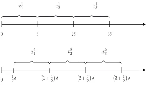
Realised kernels are based on returns that are computed on a time mesh which is started at time t = 0. Starting at t = 0 is an ad hoc choice and there may be efficiency gains possible by jittering the initial value many times and averaging the resulting collection of different realised kernel estimators. This point is made forcefully in the context of calculating realised variances by Zhang, Mykland, and A¨ıt-Sahalia (2005b). The jittering of the initial value is illustrated in Figure 1.

t

t

Figure 1: Two sets of returns. The top seriesx1_j are the conventional ones. The bottom series are the offset returns xs_j, s= 2, . . . , S. These are used to compute alternative realized autocovariances and subsampled realized kernels.

For the analysis of subsampled realised kernels it is helpful to distinguish between three types of kernels functions,k(x),withk(0) = 1 and k(1) = 0.We label the three types of kernel functions as

smooth,kinked, anddiscontinuous kernels. Representative members of these three classes of weight functions are the Parzen, the Bartlett, and the truncated kernel, respectively. Barndorff-Nielsen, Hansen, Lunde, and Shephard (2006) have shown that the class of smooth weights, which satisfy

k′_{(0) = k}′_{(1) = 0, lead to realised kernels that converges at the efficient rate, n}1/4_{. Whereas the} kinked kernels, which do not satisfy k′(0) = k′(1) = 0, lead to realised kernels that convergence at the slower rate, n1/6. The discontinuous kernels lead to inconsistent estimators as we show in Section 6.

In this paper we show that subsampling is very useful for the class of discontinuous kernels, because subsampling makes these estimators consistent and converge in distribution at rate n1/6.

In his pioneering paper, Zhou (1996) used a simple truncated kernel and gave a brief discussion of the subsampled version of his realised kernel. His estimator belongs to the class of discontinuous kernels. We will see that his estimator can be made consistent by allowing S _{→ ∞} as n_{→ ∞}, a result which is implicit in his paper, but one he did not explicitly draw out. For the class of kinked kernels, we show that subsampling is impotent, in the sense that the asymptotic distribution is the same whether subsampling is used or not. Finally, we show that subsampling is harmful when applied to smooth kernels. In fact, if the number of subsamples,S,increases with the sample size,

n, the best rate of convergence is reduced to less than the efficient one, n1/4.

Still, subsampling does provide a simple way to make use of all available data while making valid inference using realistic assumptions about the noise in tick-by-tick data. We discuss this

aspect in Section 7 and make recommendations on how to implement subsampled realised kernels in empirical work.

Our analysis is based on equally spaced data. By applying the time-change argument of Barndorff-Nielsen, Hansen, Lunde, and Shephard (2006), it follows that our results also applies to irregularly spaced data. For instance, the case whereδ corresponds to the time between every fifth transaction.

This paper has the following structure. We present the basic framework in Section 2 along with some known results. In Section 3 we derive the limit theory for subsampled realised autocovari-ances. We present our main results in Section 4. Here we derive the limit theory for subsampled realised kernels and show that subsampling cannot improve realised kernels within a very broad class of estimators. Section 5 presents some intuition for our theoretical results. In Section 6 we characterize some poorly designed kernels and show that subsampling improves upon such esti-mators. In Section 7, we given some specific recommendations on empirical implementation of subsampled realised kernels and how to conduct valid inference in this context. We present results from a small simulation study in Section 8 and an empirical application in Section 9. We conclude in Section 10 and present all proofs in an appendix.

2

Notation, definitions and background

2.1 Semimartingales and quadratic variation

The fundamental theory of asset prices says that the log-price at timet,Yt, must, in a frictionless arbitrage free market, obey asemimartingaleprocess (writtenY ∈ SM) on some filtered probability space Ω,F,(Ft)t≥T∗, P

, where T∗ ≤ 0. Introductions to the economics and mathematics of semimartingales are given in Back (1991) and Protter (2004). It is unusual to start the clock of a semimartingale before time 0, but this raises no technical difficulty and eases the exposition. We think of 0 as the start of an economic day and sometimes it is useful to use data from the previous day. Alternatively we could define γ_h(Xδ) as using data from time 0 to t by changing the range of the summation to j = H + 1 and nδ−H and then scaling the resulting estimator. All the theoretical properties we discuss in this paper would then follow in the same way as here.

Crucial to semimartingales, and to the economics of financial risk, is the quadratic variation

(QV) process of Y ∈ SM. This can be defined as [Y]t= plim N→∞ N X j=1 Ytj−Ytj−1 2 , (1)

(e.g. Protter (2004, p. 66–77) and Jacod and Shiryaev (2003, p. 51)) for any sequence of deter-ministic partitions 0 =t0< t1 < ... < tN =twith supj{tj+1−tj} →0 for N → ∞.

The most familiar semimartingales are of Brownian semimartingale type (Y ∈ BSM) Yt= Z t 0 audu+ Z t 0 σudWu, (2)

whereais a predictable locally bounded drift,σis a c`adl`ag volatility process andW is a Brownian motion. For reviews of the econometrics of this type of process see, for example, Ghysels, Harvey, and Renault (1996) and Shephard (2005). IfY _{∈ BSM}then

[Y]t=

Z t

0

σ2_udu.

In some of our asymptotic theory we also assume, for simplicity of exposition, that

σt=σ0+ Z t 0 a#_udu+ Z t 0 σ#_udWu+ Z t 0 v_u#dVu, (3)

where a#, σ# and v# are adapted c`adl`ag processes, with a# also being predictable and locally bounded andV is Brownian motion independent of W. Much of what we do here can be extended to allow for jumps inσ, following the details discussed in Barndorff-Nielsen, Graversen, Jacod, and Shephard (2006), but we will not address that here.

2.2 Assumptions about noise

We write the effects of market frictions asU, so that we observe the process

X =Y +U, (4)

and think ofY ∈ BSMas the efficient price. Our scientific interest will be in estimating [Y]t. In the main part of our work we will assume thatY ⊥⊥U where, in general,A⊥⊥B denotes thatAand

B are independent. From a market microstructure theory viewpoint this is a strong assumption as one may expect U to be correlated with increments in Y. However, the empirical work of Hansen and Lunde (2006) suggests this independence assumption is not too damaging statistically when we analyse data in thickly traded stocks recorded approximately every minute. Further, Barndorff-Nielsen, Hansen, Lunde, and Shephard (2006) show under some models of dependence between Y

and U that realised kernels are still consistent. See also Kalnina and Linton (2006).

We make a white noise assumption about the U process (U _{∈ WN}) which we assume has E(Ut) = 0, Var(Ut) =ω2, Var(Ut2) =λ2ω4, Ut⊥⊥ Us (5) for any t 6= s, where λ ∈R+_{. This white noise assumption is unsatisfactory from a number of} viewpoints (e.g. Phillips and Yu (2006)) but is a useful starting point if we think of the market frictions as operating in tick time (e.g. Bandi and Russell (2005), Zhang, Mykland, and A¨ıt-Sahalia (2005b) and Hansen and Lunde (2006)). A feature ofU _{∈ WN} is that [U]t=∞. ThusU /∈ SM and so in a frictionless market would allow arbitrage opportunities. Hence it only makes sense to add processes of this type when there are frictions to be modelled.

2.3 Some known results

Analogous to the realised autocovariances we define

γ_h(Yδ, Uδ) = nδ

X

j=1

yjuj−h, yj =Yδj−Yδ(j−1) and uj =Uδj−Uδ(j−1). From (4) we have that

γ_h(Xδ) =γh(Yδ) +γh(Yδ, Uδ) +γh(Uδ, Yδ) +γh(Uδ).

It will be useful to have the following notation γ_e(Xδ) = {γ0(Xδ),eγ1(Xδ), ...,γeH(Xδ)}⊺, where

e

γ_h(Xδ) =γh(Xδ)+γ₋h(Xδ),and introduce the analogous definitions ofγe(Yδ),eγ(Uδ),andeγ(Yδ, Uδ). In the non-subsampling case Barndorff-Nielsen, Hansen, Lunde, and Shephard (2006) derived the following helpful results.

Theorem 1 We study properties as δ _↓ 0, implying nδ → ∞. Writing M N to denote a mixed

normal distribution. Suppose that Y ∈ BSM and (3) holds, then

n1_δ/2      γ₀(Yδ)− Rt 0 σ2udu ˜ γ₁(Yδ) .. . ˜ γ_H(Yδ)      Ls →M N 0, A1×t Z t 0 σ4_udu , A1 =      2 0 _{· · ·} 0 0 4 _{· · ·} 0 .. . ... . .. ... 0 0 _{· · ·} 4     . (6)

Here Lsdenotes convergence in law stably. If, in addition,U _{∈ WN} and Y _⊥⊥U thenγ_e(Yδ, Uδ)→Ls

M N 0,2ω2_{[Y]B, where B is a (H+ 1)×(H+ 1) symmetric matrix with block structure}

B = B11 B12 B21 B22 , B22=      2 _{• • •} −1 2 • • . .. ... ... _• · · · 0 −1 2     , B11= 1 • −1 2 , B21=      0 ₋1 0 0 .. . ... 0 0     ,

B12=B21⊺. HereB22 is a (H−1)×(H−1) symmetric matrix.

Finally, when U ∈ WN and writingnδ=⌊t/δ⌋, for nδ≥H

E_{eγ(Uδ)}= 2ω2nδ(1,−1,0,0, ...,0)⊺, and Cov{eγ(Uδ)}= 4ω4

nδC+De

.

Here the (H+ 1)×(H+ 1) symmetric matrices C and De have block structure

C= C11 C12 C21 C22 , De = De11 De12 e D21 De22 ! ,

where the (H₋1)_×(H₋1) and (H₋1)_×2 dimensional matrices are

C22=        6 • • • • −4 6 • • • 1 ₋4 6 _{• •} 0 1 ₋4 6 _• .. . . .. ... ... ...        , C21=        1 −4 0 1 0 0 .. . ... 0 0        ,

e D22=          −7 _{• • • • •} 6 −10 • • • • −2 8 ₋13 _{• • •} 0 ₋2.5 10 ₋16 _{• •} .. . ... . .. ... ... ... 0 0 · · · −H 2 2H −3H−1          , De21=        −1 4 0 ₋3₂ 0 0 .. . ... 0 0        ,

where C12=C21⊺ and De12 =De21⊺. The 2×2 matrices C11 and De11 are C11= 1 +λ2 ₋2₋λ2 −2−λ2 5 +λ2 ,De11= −λ2/2 λ2/2 + 1 λ2/2 + 1 −λ2/2−7/2 .

3

Subsampled realised autocovariances

The subsampled realised autocovariances are defined by

γs_h(Xδ) = nδ

X

j=1

xs_jxs_j−h, xs_j =X_{δ(j+(s−1)/S)}−X_{δ(j+(s−1)/S−1)},

for s = 1, . . . , S, where xs_j are intraday returns over intervals of length δ, see Figure 1 for an illustration. For each of theS subsamples the realised kernel is given by,

˜ Ks(Xδ) =γs0(Xδ) + H X h=1 k h₋1 H γs_h(Xδ) +γs₋h(Xδ) , and we define thesubsampled realised kernel as

˜ K(Xδ;S) = 1 S S X s=1 ˜ Ks(Xδ) =γ0(Xδ;S) + H X h=1 k h_H−1 γ_h(Xδ;S) +γ₋h(Xδ;S) . Here γ_h(Xδ;S) = 1 S S X s=1 γs_h(Xδ).

Notice that the subsampled realised kernel computes returns over intervals of length δ but uses prices measured every δ/S periods. Hence this statistic works the database of high frequency returns more intensively than each of the realised kernels, ˜Ks_(X

δ). While the sample size used to construct each of the realised kernels is nδ, the effective sample size used by the subsampled realised kernel, ˜K(Xδ;S),is n=S×nδ.

3.1 General theory

The extension of the terms involving noise to the subsampling case is straightforward under

U _{∈ WN}, as the market microstructure terms, Ut, are uncorrelated (actually independent) cross subsamples. This implies

e γ(Yδ, Uδ;S)→LsM N 0,2ω 2 S [Y]B , (7)

E{eγ(Uδ;S)}= 2ω2nδ(1,−1,0,0, ...,0)⊺, (8) Cov_{eγ(Uδ;S)}= 4ω4 S nδC+De . (9)

The contributions from the ˜Dmatrix are known as end-effects because they are tied to theSfirst and the S last observations. For most estimators, this term does not show up in the asymptotic variance because it is of lower order than the other terms, such as those associated with the C

matrix. The only exception is when the estimator is based on a smooth kernel and a fixed S.

However, the end effects are also negligible in this case, because it follows from Barndorff-Nielsen, Hansen, Lunde, and Shephard (2006) that their contribution to the asymptotic variance is of order

O(ω),which is known to be small in practice. For this reason, we will ignore these end effects, as it simplifies the exposition of our analyses.

We need to extend (6) to the subsampling case. This is given in the following Theorem.

Theorem 2 Suppose thatY ∈ BSMand (3) holds, then as δ↓0

n1_δ/2      γ₀(Yδ;S)− Rt 0σ2udu, e γ₁(Yδ;S) .. . e γ_H(Yδ;S)      Ls →M N 0, AS×t Z t 0 σ4_udu , where AS = 2 3        2 +S−2 _{• 0 · · ·} 1−S−2 4 + 2S−2 • . .. 0 1−S−2 4 + 2S−2 . .. .. . . .. . .. . ..        → 2 3        2 1 0 _{· · ·} 1 4 1 . .. 0 1 4 . .. .. . . .. ... ...        =A_∞, and as δ↓0 and S→ ∞ n1_δ/2      γ₀(Yδ;S)−R₀tσ2udu, e γ₁(Yδ;S) .. . e γ_H(Yδ;S)      Ls →M N 0, A_∞×t Z t 0 σ4_udu . 3.2 Comments

Key to the asymptotic distribution of the _eγ_h(Yδ) is theAS matrix. Important special cases of this result are A1 (defined in Theorem 1) and

A2=        3/2 _{• • · · ·} 1/2 3 • . .. 0 1/2 3 . .. .. . . .. ... ...        , A3= 2 3        2(1 + 1₉) _{• • · · ·} (1−1 9) 4(1 + 181) • . .. 0 (1₋ 1₉) 4(1 + ₁₈1) . .. .. . . .. . .. . ..        .

The limiting result is a good approximation even for very small S. Subsampling does improve the accuracy of the realised autocovariances, however the improvements are very modest indeed and the potential gains are almost exhausted for very small values ofS.

These matrices include a number of important special cases which have influenced the recent econometric analysis of realised volatility. The asymptotic distribution

n1_δ/2(γ₀(Yδ)−[Y]t)→LsM N 0,2t Z t 0 σ4_udu (10) appears in the work of Jacod (1994), Jacod and Protter (1998) and Barndorff-Nielsen and Shephard (2002). The extension of (10) to the subsampled case

n1_δ/2(γ₀(Yδ;S)−[Y]t)→LsM N 0,4 3 1 + 2S −2_tZ t 0 σ4_udu , (11)

is in Zhang, Mykland, and A¨ıt-Sahalia (2005b). Note that 2₃ 2 +S−2 _{falls from 2 to 4/3 as S} rises from 1 to infinity, so

n1_δ/2(γ₀(Yδ;S)−[Y]t)→LsM N 0,4 3t Z t 0 σ4_udu , asS, nδ→ ∞. (12)

So in the absence of noise, the subsampled realised variance, γ₀(Yδ;S), produces a slightly more precise estimator than the realised variance,γ₀(Yδ), by exploiting more of the data. Goncalves and Meddahi (2004) and Zhang, Mykland, and A¨ıt-Sahalia (2005a) have studied Edgeworth expansions of these types of results, while the former also derived a bootstrapped version to improve the finite sample performance of the feasible version of the theory.

4

Subsampled realised kernel

In this section, we study subsampled realised kernels based on smooth and kinked kernel functions. Specifically, we require thatk(s) is continuous and twice differentiable on [0,1] and thatk(0) = 1 and k(1) = 0.Naturally, the derivatives at the end points are defined by

k′(0) = lim x↓0 k(x)₋k(0) x and k′(1) = limx↑1 k(1)₋k(x) 1₋x .

In the framework without subsampling, Barndorff-Nielsen, Hansen, Lunde, and Shephard (2006) showed that

k′(0) = 0 and k′(1) = 0, (13)

is a necessary condition for a realised kernel to have the best rate of convergence, and this property is also key for subsampled realised kernels. So we shall refer to kernels that satisfy (13) as smooth, and we usekinked to refer to the kernels that violate (13).

In some of our proofs it is convenient to extend the support of the kernel functions beyond the unit interval, using the conventions: k(x) = 0 forx >1 andk(−x) =k(x).

Barndorff-Nielsen, Hansen, Lunde, and Shephard (2006) showed that kernel functions of the type just described, can be used to produce consistent estimators with mixed Gaussian asymptotic distributions. These results do not require any subsampling. It is therefore interesting to analyze whether there are any gain from subsampling realised kernels or not. Perhaps surprisingly we find that subsampling is harmful or, at best, impotent, for realised kernels that are based on smooth or kinked kernel functions.

Below we formulate limit results for subsampled realised kernels using the notation

k0_•,0 = Z 1 0 k(x)2dx, k_•1,1 = Z 1 0 k′(x)2dx, k_•2,2 = Z 1 0 k′′(x)2dx,

and it is convenient to introduce the notation

ξ= ω 2 q tR₀tσ4 udu and ρ= Rt 0σ2udu q tR₀tσ4 udu ,

to simplify the expressions for the asymptotic variance.

Theorem 3 For large H and n the asymptotic distributions of

˜

K(Yδ;S)−

Z t

0

σ2_udu, K˜(Yδ, Uδ;S) + ˜K(Uδ, Yδ;S), and K˜(Uδ;S),

are mixed Gaussian with mean zero and asymptotic variances given by

4H nδ k0_•,0t Z t 0 σ4_udu, (14) 8ω2 Z t 0 σ2_uduk_•1,1H−1 S (15) 4ω4nδ k′(0)2+k′(1)2 H−2+k2_•,2H−3S. (16)

respectively. Furthermore, K˜(Xδ;S)−R₀tσ2udu is mixed Gaussian with a zero mean and variance

4k_•0,0t Z t 0 σ4_udu    H nδ + 2ξρk_•1,1H−1+ξ2nδ h k′(0)2+k′(1)2 H−2+k2_•,2H−3i S   . (17)

A very interesting observation is that subsampling has no impact on the first term, (14). The implication is that the asymptotic distribution of the realised kernel, ˜K(Yδ),is identical to that of the subsampled realised kernel ˜K(Yδ;S).So despite the fact that subsampling lowers the variance of the individual realised autocovariances, ˜γ_h(Yδ),the variance of the realised kernel is unaffected. The reason is that subsampling introduces positive correlation between ˜γ_h(Yδ;S) and ˜γh+1(Yδ;S)

that exactly offsets the reduction in the variance of the realised autocovariances. This follows from the fact that

[AS]i,i+ [AS]i,i−1+ [AS]i−1,i= 2 3

4 + 2S−2+ 2(1₋S−2) = 4, i >1,

does not depend on S.

Subsampling does have an effect on the terms that are due to noise, (15) and (16), where the contribution to the asymptotic variance is reduced by a factor ofS.So it is (15) and (16) that will characterize the gains from increasing the sample size by a factor of S.

The most obvious generalisation of Barndorff-Nielsen, Hansen, Lunde, and Shephard (2006) is to think of the case whereS is fixed and we allow H to increase withnδ.When (13) holds, we can follow Barndorff-Nielsen, Hansen, Lunde, and Shephard (2006) and set H = c(ξnδ)1/2. Then we obtain the result that

n1_δ/4 ˜ K(Xδ;S)− Z t 0 σ2_udu Ls →M N ( 0,4ω t Z t 0 σ4_udu 3/4 ck_•0,0+ 2c− 1_ρk1,1 • +c−3k2•,2 S !) ,

which Barndorff-Nielsen, Hansen, Lunde, and Shephard (2006) saw was the best rate possible for this problem. Whether or not (13) holds, when we setH =c(ξnδ)2/3 we have

n1_δ/6 ˜ K(Xδ;S)− Z t 0 σ2_udu Ls →M N " 0,4ω4/3 t Z t 0 σ4_udu 2/3 ck_•0,0+ k′(0) 2_+k′₍₁₎2 c2_S # .

HereS plays a relatively simple role, reducing the impact of noise — by in effect reducing the noise variance from ω2 to ω2/√S. If (13) does hold then we get the very simple result that

n1_δ/6 ˜ K(Xδ;S)− Z t 0 σ2_udu Ls →M N ( 0,4ck_•0,0ω4/3 t Z t 0 σ4_udu 2/3) .

The latter result is interesting, for it has no asymptotic gains at all from subsampling.

Until now, we have stated asymptotic results using nδ,even though the subsampled statistics are based on a larger sample size – one that is aboutS times larger. Next we make the transition to the effective sample size.

4.1 Effective Sample Size

For the purpose of discussing the effects of subsampling it is useful to make the comparison in terms of the effective sample size,n=nδS.This makes it explicit that a largerS reduces the sample size,

nδ, that is available for each to the realised kernels. Then we ask if it is better to increase nδ or

S for a given n — i.e. should we split time into lengthy returns and lots of subsampling, or use shorter returns and less subsampling.

4t Z t 0 σ4_udu " HS n k 0,0 • + 2ξρk_•1,1 HS +nξ 2 ( k′₍₀₎2_+k′₍₁₎2 (HS)2 +S k2_•,2 (HS)3 )# . (18)

Here HS appears in the variance expression in a way that is almost identical to H when there is no subsampling (S = 1). The only difference is the impact on the last term. This term vanishes when k′(0) =k′(1) = 0 does not hold, because the second last term is thenO n/(SH)2 whereas the last term is onlyO H−1O n/(SH)2.This feature of the asymptotic variance holds the key to the different results we derive for smooth and kinked kernels.

4.2 Kinked Kernels: When k′_{(0) =}k′_{(1) = 0 does not hold}

When (13) does not hold the asymptotic variance is given by 4t Z t 0 σ4_udu ( HS n k 0,0 • + 2ξρk_•1,1 HS +nξ 2k′(0)2+k′(1)2 (HS)2 ) .

While this expression depends on the productHS,it is invariant to the particular values of H and

S,though we do need H→ ∞ to justify the terms,k_•0,0,k_•1,1,etc. We have the following result.

Theorem 4 (i) If SH=c(ξn)2/3 we have n1/6 ˜ K(Xδ;S)− Z t 0 σ2_udu Ls →M N 0,4ω4/3 t Z t 0 σ4_udu 2/3 ck_•0,0+k′(0) 2_+k′₍₁₎2 c2 ! , (19)

as n→ ∞,so long as H increase with n. (ii) The asymptotic variance is minimised by

c= 2k′(0) 2_+k′₍₁₎2 k_•0,0 1/3 , and 6ck0_•,0ω4/3 t Z t 0 σ4_udu 2/3

is the lower bound for the asymptotic variance.

An interesting observation is that the asymptotic distribution (19) is not influenced by S,not even the rate of growth in S. All that matters is that H grows and that HS grows at the right rate. The implication is that there are no gains from subsampling whenk′(0)2+k′(1)2 6= 0. So we might as well set S= 1 and use the realised kernel that does not require any subsampling.

The second part of Theorem 4 shows that

ck_•0,0= 6h2 k_•0,02k′(0)2+k′(1)2 i1/3 controls the asymptotic efficiency of estimators in this class.

Example 1 The Bartlett kernel, k(x) = 1₋x, has k0_•,0 = 1/3 and k′₍₀₎2_+k′₍₁₎2 _{= 2, so that} 6ck0_•,0 = 2_·121/3 _≃4.58,whereas the quadratic kernel,k(x) = 1₋2x+x2,is more efficient, because it has k_•0,0 = 1/5 and k′(0)2+k′(1)2 = 4,so that 6ck_•0,0 = 12_·5−2/3 _≃4.10.

4.3 Smooth Kernels: When k′_{(0) =}k′_{(1) = 0 holds}

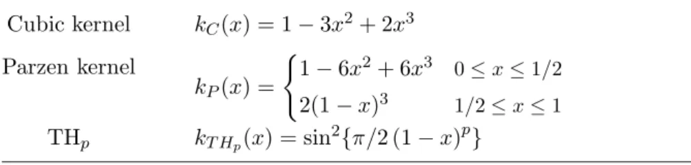
In this Section we consider smooth kernel functions. Some examples of smooth kernel functions are given in Table 1, where kth₁(x) = sin2

_π

2(1−x) = [1−cos{π(1−x)}]/2 = {1 + cos (πx)}/2 is the Tukey-Hanning kernel.

Table 1: Some smooth kernel functions. Cubic kernel kC(x) = 1−3x2+ 2x3 Parzen kernel kP(x) = ( 1₋6x2_{+ 6x}3 _0≤x≤1/2 2(1−x)3 1/2_≤x_≤1 THp kT Hp(x) = sin 2_{{π/2 (1−x)}p }

We know from Barndorff-Nielsen, Hansen, Lunde, and Shephard (2006) that the rate of con-vergence of realised kernels improves when k′(0) =k′(1) = 0. This smoothness condition will also improve the rate of convergence for subsampled realised kernels. For smooth kernel functions, the asymptotic variance is given by

4t Z t 0 σ4_udu ( HS n k 0,0 • + 2ξρk_•1,1 HS +ξ 2_nS k•2,2 (HS)3 ) . (20)

Because the last term is multiplied withS it is evident that the asymptotic distribution will depend on whetherS is constant or increases withn. This is made precise in the following Theorem.

Theorem 5 (i.a) When S is fixed we set HS=c(ξn)1/2 and have

n1/4 ˜ K(Xδ)− Z t 0 σ2_udu Ls →M N " 0,4ω t Z t 0 σ4_udu 3/4 ck0_•,0+2ρ c k 1,1 • + S c3k 2,2 • # . (21)

(i.b) When S =anα _{for some 0< α <2/3,we set HS =c(ξn)}1/2_nα/4 _{and have} n1−α/4 2 ˜ K(Xδ;S)− Z t 0 σ2_udu Ls →M N " 0,4ω t Z t 0 σ4_udu 3/4_n ck_•0,0+ a c3k 2,2 • o# .

(ii) Whether S is constant or not, the asymptotic variance is minimized by

HS= (ξn)1/2 v u u tρk1•,1 k_•0,0 ( 1 + s 1 + 3Sk 0,0 • k•2,2 (ρk1_•,1)2 ) ,

and the lower bound is

n−1/2ω t Z t 0 σ4_udu 3/4 g(S), (22)

where g(S) = 16 3 q ρk_•1,1k_•0,0          1 v u u t1+ s 1+3Sk0•,0k 2,2 • (ρk_•1,1)2 + v u u t_{1 +} s 1 + 3Sk 0,0 • k2•,2 (ρk_•1,1)2          . (23)

Remark. In (i.b) we impose α < 2/3. The reason is that H ∝ n1/2+α/4−α _{= n}(1−3

2α)/2 and we

need (1₋ 3₂α)/2>0 to ensure thatH grows with n.

The relative efficiency in this class of estimators is given from g(S),and we have the following important result for subsampling of smooth kernels

Corollary 1 The asymptotic variance of K˜(Xδ;S) is strictly increasing in S.

The implication is that subsampling is always harmful for smooth kernels. Furthermore, (i.b) shows that there is an efficiency loss from allowing S to grow with n. See Table 2 for the values of

g(S) for some selected kernel functions.

Another implication of Theorem 5 concerns the best way to sample high frequency returns. This result is formulated in the next corollary and will require some explanation.

Corollary 2 The asymptotic variance, (22), as a function of ρ, is minimized for ρ= 1.

The parameter ρ=R₀tσ2_udu/

q

tR₀tσ4_{du may appear to be fixed, which would make the} Corol-lary rather uninteresting. However, ρ is not fixed because the integrated quarticity, R₀tσ4du, de-pends on the sampling scheme. Rather than equidistant sampling in calendar time we can generate the sampling times by,

tj =t×τ j n , j= 0,1, . . . , n.

Here τ is simply a time changing mapping (for the unit interval), i.e. τ(0) = 0, τ(1) = 1, and

τ is monotonically increasing, so that 0 = t0 ≤ t1 ≤ · · · ≤ tn = t. A change of time does not affect R₀tσ2_udu but does influence the integrated quarticity R₀tσ4_udu, see e.g. Mykland and Zhang (2006). A particularly interesting sampling scheme is that known asbusiness time sampling, see e.g. Oomen (2005, 2006). Under this sampling scheme intraday returns are sampled in a way that makes them homogeneous, i.e. Rti

ti−1σ

2

udu = n−1

Rt

0 σ2udu. The integrated quarticity is minimized under this sampling scheme as was shown by Hansen and Lunde (2006, p. 135), where the minimum has tR₀tσ4_{du =} Rt

0σ2udu

2

, implying ρ = 1. It follows that the τ for business time sampling,

τbts say, must solve R₀t×τ(s)σ2_udu = s×R₀tσ2_udu. So by the implicit function theorem we have

τ′bts(s) ∝ 1/σ2(˜s), where ˜s=t×τbts(s). Thus, under this scheme the returns are sampled more

frequently when the volatility is high and less frequent when the volatility is low. In general we have ρ≤1 and Corollary 2 shows that business time sampling (ρ= 1) is the ideal sample scheme

(for a given sample size, n). Sampling in business time is infeasible because τbts depends on

the unknown volatility path. In practice, tick time sampling, where sampling occurs every fixed number of transactions, seems to be a better proxy for business time sampling than is calendar time sampling. In this situation, Corollary 2 states that it is better to sample returns in tick time. Given S and ρ it is easy to compute the optimalH,asH =cS(ξn)1/2 for this class of kernels, where cS=S−1 v u u tρk1•,1 k_•0,0 ( 1 + s 1 + 3Sk 0,0 • k•2,2 (ρk1_•,1)2 ) . (24)

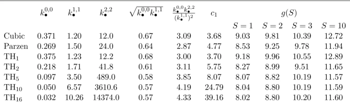
Table 2: Key quantities for some smooth-continuous kernels.

k_•0,0 k1_•,1 k2_•,2 pk0_•,0k1_•,1 k0•,0k 2,2 • (k•1,1)2 c1 g(S) S= 1 S= 2 S= 3 S = 10 Cubic 0.371 1.20 12.0 0.67 3.09 3.68 9.03 9.81 10.39 12.72 Parzen 0.269 1.50 24.0 0.64 2.87 4.77 8.53 9.25 9.78 11.94 TH1 0.375 1.23 12.2 0.68 3.00 3.70 9.18 9.96 10.55 12.89 TH2 0.218 1.71 41.8 0.61 3.11 5.75 8.27 8.99 9.51 11.65 TH5 0.097 3.50 489.0 0.58 3.85 8.07 8.07 8.82 10.19 11.57 TH10 0.050 6.57 3610.6 0.57 4.19 24.79 8.04 8.80 10.19 11.59 TH16 0.032 10.26 14374.0 0.57 4.33 39.16 8.02 8.80 10.20 11.60

Key quantities for some smooth kernels. Key is g(S) that measures the relative efficiency in this class of estimators. Here computed for the case with constant volatility (ρ = 1) such that these numbers are comparable with the maximum likelihood estimator that has g= 8.00. No subsampling

(S = 1)produces the best estimator and kernels with a relative largek0_•,0k_•2,2/(k_•1,1)2 _{tend to be more}

sensitive to subsampling.

In Table 2 we present key quantities for some smooth kernels. Perhaps the most interesting quantitiy is g(S) of (23), as it enable us to compare the relative efficiency across estimators. In Table 2 we have computed g(S) for the case where ρ= 1. Sog(S) can be compared to 8.00 which is the corresponding constant for the maximum likelihood estimator in the parametric version of the problem. We see that most kernels are only slightly less efficient than the maximum likelihood estimator, TH16 almost reaching this lower bound. Comparing g(S) for different degrees of sub-sampling, reminds us thatS = 1 (no subsampling) yields the most efficient estimator. The larger the value of k0_•,0k_•2,2/(k_•1,1)2 the more sensitive is the kernel to subsampling.

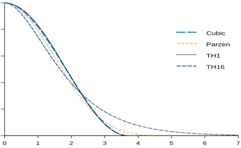
In Figure 2 we have plotted some smooth kernel functions,k(x/c1) using their respective optimal value for c1,see Table 2. We see that the TH1 kernel is almost identical to the cubic kernel. The TH16 kernel is somewhat flatter, putting less weight on realised autocovariance of lower order and higher weight on realised autocovariance of higher order. The Parzen kernel is typically between TH1 and TH16.

0.0 0.2 0.4 0.6 0.8 1.0 0 1 2 3 4 5 6 7 Cubic Parzen TH1 TH16

Figure 2: Plots of some selected smooth kernels, k(x/c1), using their repective optimal value of c whenS = 1.

While the smooth kernels improve the rate of convergence over the kinked kernels, the im-provements may be modest in finite samples. The reason is the following. When the noise is small the optimal H is small, andH may actually be quite similar for kinked and smooth kernels. For instance with ξ = 0.01 and n = 780, which corresponds to sampling twice per minute on a typical trading day, the Bartlett kernel has cBartlett(ξn)2/3 = 9.00 whereas the cubic kernel has

cCubic(ξn)1/2 = 10.78. So in this case the two types of estimators are rather similar and despite

the fact that HBartlett grows at the faster raten2/3, the cubic kernels includes more lags in this

situation. Consistent with this observation, Bandi and Russell (2006) find that the finite sample properties of kinked and smooth kernels are quite similar, although they do report some gains from the smooth kernels.

5

Intuition: Subsampled realised kernels are realised kernels

A closer inspection of subsampled realised kernels reveals that these can approximately be repre-sented by a realised kernel. Lemma A.1 in the appendix shows that

γ_h(Xδ;S)≃ S_X−1

s=−S+1

kB _SsγSh+s(Xδ/S), where kB(x) = 1− |x|,

where the approximation is due to minor end-effects. See the proof of Lemma A.1 for details. The implication is that ˜ K(Xδ;S) ≃ S−1 X s=−S+1 kB _Ss γ_s(Xδ/S) + H X h=1 k h_H−1 S X s=−S kB _Ss γSh+s(Xδ/S) +γ₋Sh−s(Xδ/S)

= HS

X

h=0

kS h_HS−1γ˜Sh+s(Xδ/S).

So a subsampled realised kernel is a realised kernel simply operating on a higher frequency (setting aside minor end-effects). The implied kernel weights, kS(_HSh ), h = 1, . . . , SH, are simply convex combinations of neighboring weights of the original kernel,

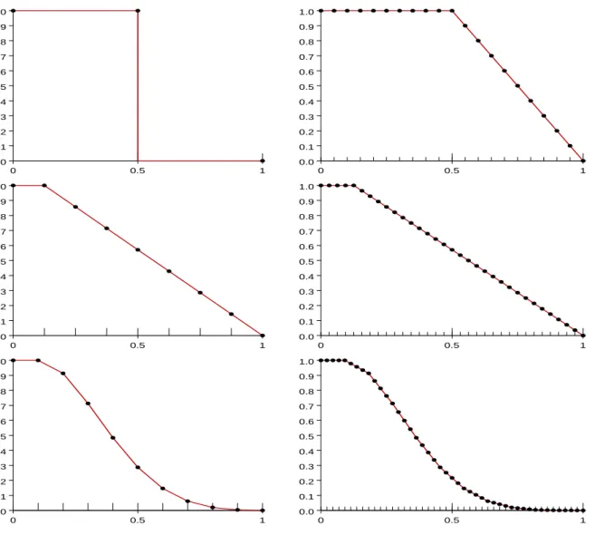
kS _HShs= S_S−sk _Sh+_Ssk h+1_S , h= 0, . . . , H, s= 1, . . . , S. (25) This provides intuition for the theoretical results we have established for subsampled realised ker-nels. Truncated (Zhou) 0.0 0.1 0.2 0.3 0.4 0.5 0.6 0.7 0.8 0.9 1.0 0 0.5 1 0.0 0.1 0.2 0.3 0.4 0.5 0.6 0.7 0.8 0.9 1.0 0 0.5 1 Bartlett 0.0 0.1 0.2 0.3 0.4 0.5 0.6 0.7 0.8 0.9 1.0 0 0.5 1 0.0 0.1 0.2 0.3 0.4 0.5 0.6 0.7 0.8 0.9 1.0 0 0.5 1 TH2 0.0 0.1 0.2 0.3 0.4 0.5 0.6 0.7 0.8 0.9 1.0 0 0.5 1 0.0 0.1 0.2 0.3 0.4 0.5 0.6 0.7 0.8 0.9 1.0 0 0.5 1

Figure 3: The effects of subsampling some kernels. The left panels display the original kernel func-tions and the right panels display their implied kernel funcfunc-tions that are induced by subsampling. For the truncated (discontinuous) kernel the two are very different. So subsampling makes an important difference in this case. For the (kinked) Bartlett kernel the two are virtually identical, which suggests that subsampling has no effect on this kernel. Finally, for the smooth kernel in the lower panels subsampling has only a small effect by making the kernel function piecewise linear.

The left panels display the original kernel functions and right panels display the implied kernel functions. The first kernel is the truncated kernel (H = 1),where we see that subsampling leads to a substantially different implied kernel function. For the kinked Bartlett kernel we see that subsampling leads to the same kernel function. For the smooth TH2 kernel function, we see that the original and implied kernel functions are fairly similar, however subsampling does impose some piecewise linearity which is the reason that subsampling of smooth kernels increases the asymptotic variance.

The connection between subsampled realised kernels and realised kernels is perhaps not too surprising, because Bartlett (1950) motivated his kernel with the subsampling idea, see also An-derson (1971, p. 512) and Priestley (1981, pp. 439–440), where the latter have a discussion of end effects. Similar relations are found between estimators of the long-run variance, for instance Politis, Romano, and Wolf (1999) noted that the subsample-estimator of Carlstein (1986) is identical to the moving block bootstrap estimator and the Jackknife estimator in this context. An interesting observation from our analysis is that subsampled kinked kernels are essentially unaffected, whereas subsampling changes the shape of smooth kernels in an unfortunate way.

6

The case with discontinuous kernel functions

In this section we consider the kernel functions we have labelled as discontinuous kernels. Such kernels lead to estimators with poor asymptotic properties. We shall see that subsampling can substantially improve such estimators, making them consistent with mixed Gaussian distributions. So for such kernels, subsampling is a saviour.

Lemma 1 Let K˜w(Xδ) =PHh=0wh˜γh(Xδ), where H=o(n) (possibly constant). Then

w0= 1 +o(1) and w0−w1 =o(n−1),

are necessary conditions for EK˜w(Xδ)−

Rt 0σ2udu →0; and H X h=0 (wh+1−2wh+wh−1)2 =o(n−1), (26)

is a necessary condition for VarK˜w(Xδ)−

Rt

0σ2udu

→0, where we set wH+1= 0 andw−1 =w0. The lemma shows that realised kernels using a fixed H cannot converge to R₀tσ2_udu in mean squares, because such estimators will not satisfy (26).

Now consider the case where we construct wh from a kernel function and letH→ ∞, as we did in the previous section. In this situation it is clear that any discontinuous kernel will violate (26),

because n H X h=0 (wh+1−2wh+wh−1)2 ≃n×J2, where J2= X xj∈Dk lim x↑xj k(x)−lim x↓xj k(x) 2 .

Here _Dk is the set of discontinuity points for k(x).

Next, we consider the truncated kernel which does not satisfies (26). We will see that subsam-pling this kernel produces an estimator that is consistent and mixed Gaussian. This is true whether

H is finite or is allowed to grow with the sample size.

6.1 Zhou (1996) estimator

First we will look at estimators which are thought of as having H fixed and allowing the degree of subsampling to increase. This is outside the spirit of the realised kernels of Barndorff-Nielsen, Hansen, Lunde, and Shephard (2006) which needH to get large with nδ for consistency, however it is close to the important early work of Zhou (1996) and is strongly intellectually connected to the influential work on two scale estimators by Zhang, Mykland, and A¨ıt-Sahalia (2005b).

The Zhou (1996) estimator can be written as

γ₀(Xδ;S) +eγ1(Xδ;S)

which is the subsampled realised kernel based on the truncated kernel function usingH = 1. Zhou (1996) noticed that the variance of his estimator was of order O(_nS

δ) +O( 1

S) +O( nδ

S2), but did not

realize that by allowing S to increase with nδ his estimator is consistent. In fact, in a subsequent paper Zhou stated that his subsampled realised kernels was inconsistent, see Zhou (1998, p. 114). The following Theorem gives its asymptotic distribution.

Theorem 6 Suppose S=c3_n2 δ, then as nδ→ ∞ n1_δ/2 γ₀(Xδ;S) +γe1(Xδ;S)− Z t 0 σ2_udu Ls →M N 0,16 3 Z t 0 σ4_udu+ 8ω4/c3 .

This asymptotics is not particularly attractive for its seeming n1_δ/2 rate of convergence hides the fact that it assumes massive databases in order to allow S to increase rapidly withnδ. A more interesting way of thinking about this estimator is in terms of the effective sample size

n=S×nδ.

Lemma 2 If S=c(ξn)2/3 then the Zhou estimator has n1/6 γ₀(Xδ;S) +γe1(Xδ;S)− Z t 0 σ2_udu Ls →M N 0, ω4/3 t Z t 0 σ4_udu 2/3 16 3c+ 8 c2 ! .

The minimum asymptotic variance is

8√33 |{z} ≃11.54 ω4/3 Z t 0 σ4_udu 2/3 , with c=√33.

The relationship S =c(ξn)2/3, which implies that S ∝n2_δ, gives the impression that this esti-mator will require massive subsampling to work, however if the noise is small this is not necessarily the case.

An interesting feature of the Zhou estimator is that its asymptotic variance is of the form obtained by the kinked non-subsampled realised kernels, i.e. ones which do not satisfy the k′(0) =

k′(1) = 0 condition.

Example 2 Suppose n corresponds to using prices every 1 second for a whole trading day on the NYSE, so n= 23,400. If ω2 = 0.001 and tR₀tσ4_udu = 1, which is roughly right in empirical work from 2004 for thickly traded stocks, then for the Zhou estimator the optimal degree of subsampling isS _≃25 so that nδ ≃920. Thus the procedure is suggesting subsampled 25 second returns. Hence

the degree of subsampling is rather modest. In 2000, ω2 _{= 0.01 and} Rt

0σ4udu = 1 would be more

reasonable, in which case S = 118 and nδ = 198, which corresponds to returns measured every

roughly 2 minutes.

6.2 2-lag flat-top Bartlett estimator

A natural extension of Zhou (1996) is to allow H to be larger than one but fixed. The theory of realised kernels suggested this may well produce more efficient estimators, which we now show is true.

Lemma 3 Let w0 =w1 = 1 and w2 = 1/2.With S =c(ξn)2/3 we have n1/6 γ₀(Xδ;S) +γe1(Xδ;S) + 1 2eγ2(Xδ;S)− Z t 0 σ2_udu Ls →M N 0, ω4/3 t Z t 0 σ4_udu 2/3 20 3 c+ 2 c2 ! ,

and the minimum variance is

10p3 3/5 | {z } ≃8.43 ω4/3 Z t 0 σ4_udu 2/3 , with c=p3 3/5.

The constant in the asymptotic variance is here reduced from about 11.54 to 8.43. So this estimator is quite a bit more efficient than the Zhou estimator.

In the previous Theorem we added w2 = 1/2 times ˜γ2(Xδ) to Zhou’s estimator, which led to a reduction of the asymptotic variance. Now we proceed by adding additional realised autocovariances to Zhou’s estimator, using the Bartlett weights,wh =k(h_H−1), h= 2, . . . , H. An interesting question is what happens as we increase H further? For moderately large H we have that

n1/6 ˜ K(Xδ)− Z t 0 σ2_udu

has an asymptotic variance of approximately 4 3{2 + (H+ 1)}c Z t 0 σ4_udu+ 8ω 4 c2_H2. This suggests c3 = 12ω 4 H3Rt 0σ4udu +o(1),

so the asymptotic variance (using 4₃121/3_{+ 8/12}2/3 _{= 2}√3

12) is 2√312 | {z } ≃4.58 ω4/3 Z t 0 σ4_udu 2/3 +o(1).

So we achieve an additional reduction of the asymptotic variance. Not surprisingly, this is the asymptotic variance of the Bartlett realised kernel applied to a sample of size n when H ∝ n2/3, see Example 1. Here, by allowing H to grow we approach the situation with kinked kernels so we observe the eventual impotence of subsampling – a property we have shown holds for all kinked kernels. Hence as H gets large the optimal degree of subsampling rapidly falls and the best thing to do is simply to run a Bartlett realised kernel on the data without subsampling, i.e. takenδ=n. Figure 4 shows the implied kernel functions that are generated by subsampling Zhou’s estimator (H = 1) and the two estimators that have been enhanced by adding Bartlett weights. The relative asymptotic efficiency for these estimators are simply given by k_•0,0 of the implied kernel. From Figure 4 it is evident that k_•0,0(H = 1) > k_•0,0(H = 2) > k_•0,0(H = ∞) which explains that the asymptotic variance of this estimator is decreasing inH.

6.3 Relationship to two scale estimator

The main idea in the two scale estimator of Zhang, Mykland, and A¨ıt-Sahalia (2005b) was to use

γ₀(Xδ;S) and bias correct it using the estimator ˆ

ω2 = γ0(Xδ/S) 2n

which exploits very high frequency returns over time intervals of length δ/S. Their results are reproved here, exploiting our previous results to make the proofs very short.

0 1/3 1/2 2/3 1 0 1/2 1 H=1 H=2 H=oo

Figure 4: The implied kernels that arise from subsampling some simple kernels. H = 1 corresponds to the subsampled version of Zhou’s estimator; H = 2 is that for Zhou’s estimator after adding 1/2˜γ₂(Xδ); and H =∞ (here approximated by H = 18) illustrates the implied kernel for Zhou’s estimator that is enhanced by an increasing number of Bartlett-weighted realised autocovariances.

We set

S =c3ξ2n2_δ, or equivalently S =c(ξn)2/3,

which imposes the optimal rate forS in this context.

Theorem 7 With S=c(ξn)2/3 _{we have} n1/6 γ₀(Xδ;S)−nδ2ω2− Z t 0 σ2_udu Ls →M N ( 0, ω4/3 t Z t 0 σ4_udu 2/3 4 3c+ 4 1 +λ2 c2 ) . (27) This asymptotic result is infeasible in the sense that γ₀(Xδ;S)−nδ2ω2 is not an estimator of

Rt

0σ2udu, because it involves the unknown parameter,ω2.Shortly we will analyse the feasible esti-mator, where ˆω2=γ₀(X_δ/S)/2nis substituted for ω2.The following result address the asymptotic consequences of this substitution.

Theorem 8 With S=c(ξn)2/3 _{we have} n1/6 ( 1 S PSnδ j=1 Ujδ/S −U(j−S)δ/S 2 −nδ2ω2 1 S PSnδ j=1 Ujδ/S−U(j−1)δ/S 2 −nδ2ω2 ) Ls →N 0, 4ω 4 c2_ξ4/3 1 +λ2 λ2 λ2 1 +λ2 .

The structure of the asymptotic covariance matrix can now be exploited to eliminate the nui-sance parameter, λ2.The implication is

n1/6    1 S Snδ X j=1 U_jδ/S−U_(j−S)δ/S2₋ 1 S Snδ X j=1 U_jδ/S−U_(j−1)δ/S2    Ls →N 0, 8ω 4 c2_ξ4/3 ,

allowing γ₀(Uδ;S)−nδ2ω2 to be replaced by γ0(Uδ;S)−nδ2ˆω2, yielding a feasible estimator which remarkably also reduces the variance compared to the infeasible estimator. This is stated next.

Theorem 9 With S=c(ξn)2/3 we have n1/6 γ₀(Xδ;S)−2nδωˆ2− Z t 0 σ2_udu Ls →M N ( 0, ω4/3 t Z t 0 σ4_udu 2/3 4 3c+ 8 c2 ) .

The minimum asymptotic variance is

2√312 | {z } ≃4.58 ω4/3 t Z t 0 σ4_udu 2/3 , with c=√312.

Thus the two scale estimator is significantly more efficient than the Zhou estimator and is as efficient as the Bartlett realised kernel with H lags where H =c(ξn)2/3. Interesting this is solely due to replacing ω2 by ˆω2 — for if we used (27) it would deliver a less efficient estimator than the Zhou estimator in the case of Gaussian noise whereλ2= 2.In effect ˆω2 plays the role of a control variable, reducing the variance of the estimator.

Example 3 (continued from Example 2). If ω2 _{= 0.001 and t}Rt

0σ4udu = 1, then S ≃ 40 and

nδ≃580. Hence the degree of subsampling is larger than that used by Zhou.

The two scale estimator by Zhang, Mykland, and A¨ıt-Sahalia (2005b) combines a subsampled realised variance with γ₀(Xδ) for some delta. So it follows from our results in Section 5 that this estimator (apart from end effects) is a realised kernel – in this case the implied kernel is a Bartlett kernel. The two scales estimator converges at raten1/6_{,whereas the related multiscale estimator by} Zhang (2006) converges at the efficient raten1/4_{.The latter combines multiple subsampled realised} variances, each using a different S.So the multiscale estimator can also be expressed as a realised kernel. In this case the implied kernel is a linear combination of Bartlett kernels using different lag lengths. Interestingly, Barndorff-Nielsen, Hansen, Lunde, and Shephard (2006) have shown that the multiscale estimator is asymptotically equivalent to the realised kernel based on the cubic kernel function, see Table 1. Not surprisingly, it can be shown that the implied kernel for the multiscale estimator is the cubic kernel.

7

Some Empirical Recommendations

So far we have worked under the assumption that the noise is of the independent type defined in (5). This assumption seems reasonable for equity returns when prices are sampled at moderate high frequencies. For instance, for the liquid stocks in the Dow Jones Industrial Average this assumption seems reasonable when applied to 1 minute returns, see Hansen and Lunde (2006). In this context, our theoretical results have shown that the best approach to estimation is to use a smooth realised kernel without any subsampling. This, conveniently, permits one to use the feasible methods for inference developed in Barndorff-Nielsen, Hansen, Lunde, and Shephard (2006). A shortcoming of

this approach is that this estimator does not make use of all available observations. For example, transactions on the most liquid stocks now take place every few seconds, but for U ∈ WN to be reasonable we can only sample every, say, 15th observation.

In this Section we discuss how to construct subsampled realised estimators that make use of all available data. We also discuss how valid inference can be made about such estimators under realistic assumptions about the noise in tick-by-tick data.

The main idea is to use a subsampled realised kernel, where S is chosen to be sufficiently large so that (5) is reasonable for a sample that only consists of every Sth observation. The asymptotic variance can be estimated from the coarsely sampled data, using the methods by Barndorff-Nielsen, Hansen, Lunde, and Shephard (2006), and this leads to valid inference that is robust to both time-dependent and endogenous noise in the tick-by-tick data.

Specifically we recommend the following procedure.

1. ChooseSsufficiently large for (5) to be a plausible assumption for a sample that only consists of everySth observation. One can check for violation of (5) by applying the diagnostics used in Hansen and Lunde (2006).

2. Construct S distinct subsamples, by jittering the initial starting point and sampling every

Sth observation. So each subsample has approximately nδ=n/S observations. 3. For each of the S subsamples, obtain estimates of ω2 _{and IQ = t}Rt

0σ4udu, and an initial estimate of IV = R₀tσ2

udu. See Barndorff-Nielsen, Hansen, Lunde, and Shephard (2006) for ways to do this. Average each of these estimators to construct the subsampled estimators, ˆ

ω2=S−1PS_s=1ωˆ2_s and IVcinitial=S−1PSs=1IVcinitial,s and IQc =S−1PSs=1IQcs.

4. Obtain an estimate, ˆH, for the optimal H, by plugging the subsampled estimates into the expression for the optimal H. Use this ˆH to compute the S realised kernels, ˜Ks_(X

skip-S), using a smooth kernel and the weights w0 = w1 = 1 and wh = k

h−1 ˆ H , for h = 2, . . . ,H.ˆ

Form their average to obtain the actual estimator,IVcfinal= ˜K(Xskip-S;S). 5. Finally, compute the conservative estimate for avarnK˜(Xskip-S;S)

o

using the finite sample expressions d VarnK˜(Xskip-S;S) o =IQ wc ′Aw× 1 nδ + 8ˆω2IVcfinal w′Bw + 4ˆω4 w′Cw×nδ, (28) wherew= (w0, w1, . . . , w_Hˆ). Here one can use that

w′Aw = 2 + 4 H

X

h=1

w′Bw = 1 + 2 H X h=2 wh(wh−wh−1)≃H−1k1_•,1, w′Cw = 4 + H X h=2 wh(6wh−8wh−1+ 2wh−2)≃H−3k_•2,2.

The variance estimate in (28) is the sum of the finite sample versions of (14-16) with S = 1.

So this expression completely ignores subsampling, and the expression is really an estimator of Var( ˜Ks(Xskip-S)). The reason is that subsampling does not reduce the noise-variance by a factor of S, unless the noise is uncorrelated across subsamples. This is unrealistic when the subsamples exploit all the tick-by-tick data. However, we still have

avarnK˜(Xskip-S;S)

o

≤avar( ˜Ks(Xskip-S)),

even if Ut ⊥⊥ Us is violated for some s6= t. So (28) is simply a robust estimator that is expected to yield a conservative estimate of the variance. It is interesting to have some notion of how conservative this estimator is.

Recall our result in Theorem 3 that avarnK˜(Yskip-S;S)

o

= avar( ˜Ks(Yskip-S)), see (14). So subsampling cannot reduce the contribution to the asymptotic variance from this term, while the contributions from the two other terms (15) and (16), potentially can be driven all the way to zero.

Consider the realised TH2 kernel. Whenρ= 1 its asymptotic variance is proportional to c1+ 2 k_•1,1 k_•0,0c −1 1 + k_•2,2 k_•0,0c −3 1 = 5.75 + 1.71 0.218 2 5.75 + 41.8 0.218(5.75) −3 ≃9.50.

Subsampling this estimator withS = 10, say, will reduce this term to a number no less than 5.75 + 1 10 1.71 0.218 2 5.75 + 1 10 41.8 0.218(5.75) −3_≃6.12.

Hence the variance reduction will be less than 36%,and even withS_{→ ∞}the reduction will be less than 40%.In practice, the reduction is likely to be much smaller, because the noise in the different subsamples is dependent. So even though (28) is a conservative estimator – it is not perversely conservative.

8

Simulation study

In this section we analyse the finite sample properties of ˜K(Xδ;S),using both a smooth TH2kernel and a kinked Bartlett kernel. We are particularly interested in the MSE of ˜K(Xδ;S),as a function of δ and S, and to see whether the simulation based results differs from our theoretical results in any significant way.

8.1 Simulated model

We consider the following SV model,

dYt=µdt+σtdWt, σt= exp (β0+β1τt), dτt=ατtdt+ dBt, corr(dWt,dBt) =ρ, where ρ is a leverage parameter. This model is frequently used for simulation is this context, see e.g. Huang and Tauchen (2005), Goncalves and Meddahi (2004), and Barndorff-Nielsen, Hansen, Lunde, and Shephard (2006).

In our simulated model, we setµ= 0.03,β₁= 0.125,α=₋0.025 andρ=₋0.3. Further, we set

β₀ =β2₁/(2α) in order to standardize E σ2

t

= 1.With this configuration the variance ofR₀tσ2

uduis comparable to the empirical results found in Hansen and Lunde (2005). For the variance of market microstructure noise we set ω2= 0.1.

8.2 Design

The process is generated using an Euler scheme based onN = 23,400 intervals, where each interval is thought to correspond to one second so that the entire interval corresponds to 6.5 hours, which is the length of a typical trading day.1 _{The volatility process is restarted at its mean valueσ}

0 = 1 every day by setting τ0= 5/2.This keeps the noise-to-signal ratio,ξ =ω2/qR₀1σ4udu,comparable across simulations. In our Monte Carlo designs we let the effective sample size, n,be either 1,560, 4,680, or 23,400, which correspond to sampling every 15, 5, or 1 seconds, respectively. So a sample with 4,680 observations, say, is obtained by including every fifth observation of the N = 23,401 simulated data points over the [0, t] interval.

8.3 Implementation of realised kernels and subsampled realised kernels

From the simulated data, X0, . . . , Xn, we define the “skip-S returns” ∆SXj = Xj −Xj−S. The subsampled realised autocovariances are computed by,

ˆ γs_h = nδ X j=1 ∆SXjS+s−1∆SX(j−h)S+s−1, s= 1, . . . , S, h=−H, . . . ,0, . . . , H, wherenδ =n/S.The subsampled realised kernel is defined by

\ ˜ K(X;S) = 1 S S X s=1 \ ˜ Ks_{(X), where K}˜\s H(X) = ˆγs0+ H X h=1 k(h_H−1) ˆγs_h+ ˆγs_−h.

So for S= 1 we simply have

\ ˜ KH(X) = ˆγ0+ H X h=1 k(h_H−1) ˆγ_h+ ˆγ_−h, where ˆγ_h= n X j=1 xjxj−h.

1_{In practice we generate intraday returns for 33}

,400 intervals, and treat the first and and last 5,000 returns as

We use our expression for the optimal choice forH. So whenS = 1 we useH_TH∗ _2,1= 5.75(ξn)1/2 for the smooth TH2 kernel andH_Bartlett∗ _,1= 3

p

12(ξn)2 _{for the kinked Bartlett kernel. The} “noise-to-signal” parameter, ξ =ω2_/qR1

0 σ4udu need not be estimated in our simulations, because ω2 is known and the integrated quarticity,R₀1σ4

udu≃N

PN

j=1σ4j/N,can be computed from the simulated data. The parameterρ=R₀1σ2_udu/qR₀1σ4

uducan be computed from the simulated volatility path. When S ≥2 the optimalH for the Bartlett kernel is simply given byH_Bartlett∗ _,S =S−1p3 _12(ξn)2_, and the TH2 kernel hasH_TH∗ _2,S =c1_S/2(ξn),where

cS=S−1

r

7.84ρ1 +√1 + 9.33S,

as defined in (24).

8.4 Simulation Results

Figure 5 shows the Monte Carlo results with the number of subsamples, S, increasing along the horizontal axis and the MSE on the vertical axis. The lines represent different sample sizes.

Consider first the results based on the Bartlett kernel. Our theoretical results in Theorem 4 dictate that these lines should be horizontal. This result is confirmed, especially for the large sample sizen= 23,400. Still, a small increase in the MSE asS increases is observed for the smaller sample sizes. The reason is that the lag length of the implied kernel, Himplied,can only attain values that are divisible by S. While the Bartlett kernel without subsampling has H∗

Bartlett,1 =

l 3 p

12(ξn)2m_, the implied Bartlett kernel has Himplied = S ×

l

S−1p3 _12(ξn)2m_{. So as S increases the implied} kernels’ Himplied is more likely to deviate from H_Bartlett∗ _,1, which causes an increase in the mean squared error. The smaller is the sample size, n, the smaller is the optimal value for H. So it is not surprising that the impact on MSE is seen earlier whenn is small. In this design, the optimal lag length, H_Bartlett∗ _,1, is about 67, 140, and 403, for n = 1,560, n = 4,680, and n = 23,400,

respectively. Though the is some variation in the optimalH across simulations because it through

ξ, depends on the simulated volatility path. The lower panels present the results for the smooth TH2 kernel. Here, our theoretical results in Theorem 5 state that the MSE is increasing in S,and this phenomenon is evident for all sample sizes. For each of the sample sizes,n= 1,560, n= 4,680,

and n= 23,400, the optimal H∗

TH2,1,is typically 72, 125, and 279, respectively. The results when

ω2 _{= 0.01 and ω}2 _{= 0.001 (not reported) are similar. Here the optimal H is smaller and this} causes subsampling to have a larger impact on the MSE. Naturally, the implied kernels must have

Himplied≥S,so that Himplied=Swhenever S≥H∗.This constraint is relevant for our simulations with small levels of noise because subsampling takes Himplied further away from its optimal value, asS increases beyond the optimalH.

n=23400 (1 sec) n=4600 (5 sec) n=1560 (15 sec) MSE 0.020 0.025 0.032 0.041 0.052 0.065 0.083 0.105 0.133 0.169 0.214 1 2 3 4 5 6 7 8 9 11 15 20 25 35 50

Number of subsamples (noise=0.1, Bartlett kernel)

n=23400 (1 sec) n=4600 (5 sec) n=1560 (15 sec)

MSE 0.020 0.025 0.032 0.041 0.053 0.067 0.086 0.109 0.139 0.177 0.225 1 2 3 4 5 6 7 8 9 11 15 20 25 35 50

Number of subsamples (noise=0.1, TH2 kernel)

Figure 5: Mean squares errors (MSEs) for subsampled realised kernels using three different sample sizes. The upper panel presents the results for the Bartlett kernel and the lower panels presents the results for the TH2kernel. For the (kinked) Bartlett kernel we see that the MSE is fairly insensitive to S, whereas the (smooth) TH2 kernel has MSEs that are slightly increasing in S.These findings are fully consistent with the theoretical results in Theorems 4 and 5.

9

Empirical study of General Electric trades

In this section we revisit the empirical application in Barndorff-Nielsen, Hansen, Lunde, and Shep-hard (2006). Our objective is to compare subsampled realised kernels with standard realised kernels and other estimators. The estimation problem is here to estimate the daily increments of [Y] for the logarithm price of General Electric (GE) shares, using high frequency transaction data carried out on the New York Stock Exchange in 2000 and in 2004. The reason that we analyse data from both periods is that the variance of the noise was around 10 times higher in 2000 than in 2004. A more detailed analysis on 29 other major stocks is provided in a Web Appendix to this paper available from www.hha.dk/_∼alunde/bnhls/bnhls.htm. This appendix also describes the exact implementation of our estimators. Precise details on the cleaning we carried out on the raw data before it was analysed are described in the web appendix to Barndorff-Nielsen, Hansen, Lunde, and Shephard (2006).

Table 3 shows Summary statistics for seven estimators. The first estimator is the realised TH2 kernel using approximate 1 minute returns. The approximate 1 minute returns are obtained by skipping a fixed number of transactions, such that the average time between observations is one minute. In 2000 we had to skip every 9.7 observations on average to construct the approximate 1 minute returns, and in 2004 we had to skip every 13.7 observations on average. The second estimator is the subsampled realised TH2 kernel. So in 2000 we have S≃9.7 and in 2004 we have S ≃ 13.7. The third estimator is the realised TH2 kernel that is based on tick-by-tick data (i.e. all available trades) and an H that is S times larger than that used by the first estimator. This estimator should be quite similar to the subsampled realised kernel, according to our results in Section 5.

The following three estimators are subsampled realised variances. These are based on returns that are sampled in calendar time, where each intraday return spans 20 minutes, 5 minutes, or 1 minute, as indicated in the subscript of these estimators. To exhaust data sampled every second, the number of subsamples areS= 1200, S = 300,andS = 60,respectively. For instance, the estimator [X5 minutes; 300] is the average of 300 realised variances, where each of the realised variances are based on 5 minute intraday returns, simply changing the initial place that prices are recorded by one second. The last estimator, TSRV(K, J), by A¨ıt-Sahalia, Mykland, and Zhang (2005), is the two-scale estimator that is designed to be robust to deviations from i.i.d. noise. Here we use their

Table 3: Summary statistics for subsampled [Y] estimators, GE.

Mean Std. (HAC) H ρ([cY],Ke) acf(1) acf(2) acf(5) acf(10) Sample period: 2000

Modified Tukey-Hanning kernel(He =cn1/2₎ e

Kth2

w (Xap. 1 min) 4.747 3.216 (6.133) 6.558 1.000 0.43 0.25 0.03 0.15 Subsampled Modified Tukey-Hanning kernel(H =cn1/2₎

e

Kth2

w (Xap. 1 min;S) 4.709 3.220 (6.170) 6.558 0.997 0.43 0.25 0.03 0.16 Modified Tukey-Hanning kernel (H =S_·He)

e Kth2 w (X1 tick) 4.702 2.946 (5.793) 62.44 0.986 0.46 0.27 0.05 0.13 Simple RV subsampled [X20 minutes; 1200] 4.417 3.650 (6.046) 0.894 0.26 0.17 -0.01 0.17 [X5 minutes; 300] 4.908 3.018 (5.611) 0.984 0.44 0.23 0.01 0.14 [X1 minutes; 60] 5.545 2.376 (5.167) 0.787 0.55 0.36 0.10 0.18 AMZ (2006) TSRV(K, J) 3.511 2.846 (5.265) 0.941 0.36 0.21 0.01 0.23 TSRV(K, J) -aa 4.514 3.657 (6.766) 0.941 0.36 0.21 0.01 0.23 Sample period: 2004 Modified Tukey-Hanning kernel(He =cn1/2₎

e

Kth2

w (Xap. 1 min) 0.962 0.568 (1.195) 5.723 1.000 0.34 0.32 0.28 0.08 Subsampled Modified Tukey-Hanning kernel(H =cn1/2₎

e

Kth2

w (Xap. 1 min;S) 0.954 0.561 (1.202) 5.723 0.995 0.37 0.32 0.28 0.09 Modified Tukey-Hanning kernel (H =S_·He)

e Kth2 w (X1 tick) 0.947 0.522 (1.130) 78.27 0.990 0.37 0.31 0.30 0.08 Simple RV subsampled [X20 minutes; 1200] 0.885 0.516 (1.036) 0.933 0.27 0.27 0.27 0.08 [X5 minutes; 300] 0.943 0.503 (1.088) 0.984 0.37 0.32 0.30 0.08 [X1 minutes; 60] 0.942 0.376 (0.921) 0.899 0.46 0.43 0.38 0.12 AMZ (2006) TSRV(K, J) 0.736 0.436 (0.929) 0.944 0.33 0.35 0.28 0.11 TSRV(K, J) -aa 0.946 0.560 (1.194) 0.944 0.33 0.35 0.28 0.11

Summary statistics for three types of kernel based estimators: First the realised Modified Tukey-Hanning kernel using approximate 1 minute returns. Then the corresponding subsampled kernel. Next, the kernel computed using the inefficient rate and based on all available trades, after which a version with H =He ·S

follows. Next, subsampled versions of simple RV statistics based on 20, 5 and 1 minute returns are given. For instance, the subsampled [X5 minutes; 300] calculates RV over 5 minutes, averaged over 300 times, just changing the initial place prices are recorded. The AMZ (2006) are two-scale estimators designed to be robust to deviations from i.i.d. noise. The second estimator which scales TSRV(K, J)overcome its finite sample bias.

From Table 3 we see that the estimators are very tightly correlated. The two realised kernels and the subsampled realised kernel are almost perfectly correlated, and all reported statistics are quite similar for these estimators. The two scale estimator is also quite similar to the realised kernels. Interestingly, amongst the subsampled realised variances, it is that based on 5 minute returns that is most similar to the realised kernels. This suggest that 20 minute returns leads to too much sampling error, whereas 1 minute returns are being influenced by the bias due to market microstructure noise.

Estimates of [Y] 0 2 4 6 8 10 12 1 2 3 6 7 8 9 10 13 14 15 16 17 20 21 22 27 28 29 30

Days in November 2000 (GE)

e

Kth2

(Xap. 1 min) Keth2(Xap. 1 min;S) Keth2(X1 tick)S·H∗

Estimates of [Y] 0.0 0.5 1.0 1.5 2.0 1 2 3 4 5 8 9 10 11 12 15 16 17 18 19 22 23 24 29 30

Days in November 2004 (GE)

e

Kth2

(Xap. 1 min) Keth2(Xap. 1 min;S) Keth2(X1 tick)S·H∗

Figure 6: Three estimators for the daily increments to [Y] for General Electrics in November 2000 and 2004. Triangles are the estimates of the realised kernel using roughly 1 minute returns. Diamonds are the estimates produced by the subsampled realised kernel. Circles are the estimates of the realised kernel that uses tick-by-tick returns and anH that isS times larger than that used by the first realised kernel. The intervals are the 95% confidence intervals for ˜KTH2_(X

ap. 1min).

Time series for some of these estimators are drawn in Figure 6, where we plot daily point estimates for November 2000 and November 2004. We also include the confidence intervals for

˜

KTH2(Xap. 1 min) using the method of Barndorff-Nielsen, Hansen, Lunde, and Shephard (2006). The three estimators are virtually almost identical. While the subsampled realised kernel may be slightly more precise than the moderately sampled realised kernel, ˜KTH2(Xap. 1 min), Figure 6 does not suggest there is a big difference between these two. The realised kernel that is based on