RANKED SET SAMPLING AND ITS
APPLICATION IN QUALITY CONTROL
DISSERTATION
Submitted in partial fulfillment of the
requirement for the award of the degree of
Master of Philosophy
IN
STATISTICS
BY
SURIYA JABEEN
Under the Supervision of
DR. TARIQ RASHID JAN
(Assistant Professor)Post-graduate Department of Statistics
University of Kashmir, Srinagar
(NAAC ACCREDITED GRADE ‘A’)
(2011)
Dedicated To My Parents
Since the fabric of the universe is most
perfect and the work of the most Wise
Creator, nothing at all takes place in the
Universe in which some rule of the
maximum or minimum does not appear.
My work does not only reflect my industry but is a projection of unfaltering Support
and inexorable encouragement from my supervisor Dr. Tariq Rashid Jan Assistant
professor, Department Of Statistics, University of Kashmir, without whose help my work
would have been undoubtedly Ineffectual. His erudition and profundity of thoughts has
had an inexplicable impact on my research. Even on moral front he stood firm and made
things highly flexible with his valuable suggestions and practical advices that helped tide
over the difficulties confronted in the preparation of this thesis, these laudable efforts are
duly acknowledged.
I wish to express my sincere thanks to Professor Aquil Ahmed, Head of the
Department of Statistics whose encouragement was of immense value during this study.
A special note of thanks is also due to Dr. Anwar Hassan, for his generosity and
encouragement.
The moral support offered by Dr. M.A.K Baig and Dr. Sheikh Parvaiz Ahmad
was a big inspiration for this accomplishment.
It is a great privilege for me to express my deep love and reverence to my parents,
who wished and build my future giving affection and guidance to carry on the work
which really served as a beacon light for me.
I also acknowledge the assistance, cooperation and encouragement rendered by
research scholars Mr Javid, Ms Nusrat especially Ms Saba Riyaz and Non-Teaching staff
of Statistics Department, University of Kashmir.
I am very thankful to Mr. Javid Ahmad for typing this manuscript.
The concept of ranked set sampling is a recent development that enables one to
provide more structure to the collected sample items, although the name is a bit of a
misnomer as it is not as much a sampling technique as it is a data measurement technique.
This approach to data collection was first proposed by McIntyre (1952) for situations
where taking the actual measurement for sample observations is difficult.
Since its inception with the paper by McIntyre, a good deal of attention has been
devoted to the topic in the statistical literature, particularly over the past fifteen years.
Some of this work has been geared toward specific parametric families and some has been
developed under minimal nonparametric distributional assumptions. However, many of
the important concepts and features of the ranked set sampling methodology transcend the
parametric or nonparametric categories. This dissertation is divided into five chapters.
With a comprehensive bibliography given at the end.
Chapter-I presents the basic ideas, preliminary results and presents a brief review
of ranked set sampling. Methods for obtaining ranked set samples are described and the
structural differences between ranked set samples and simple random samples are
discussed.
Chapter-II deals with the estimation of mean of exponential distribution using
moving extreme ranked set sampling. Maximum likelihood estimator and a modified
Maximum likelihood estimator are considered and their properties are studied. The method
is studied under both perfect and imperfect ranking.
Chapter-III deals with ranked set sampling with size- biased probability of
selection. Ranked set sampling with probability of selection proportional to size and errors
in ranking. In this chapter RSS is used to obtain a second-phase sample and increase the
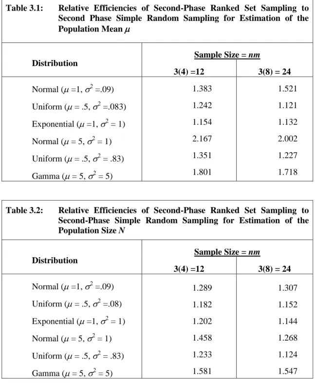
efficiency of estimators relative to simple random sampling. Estimators of the population
mean and the population size are considered. Computer simulated results are given.
Finally, ranked set sampling with errors in ranking is considered with probability of
selection proportional to size.
Chapter-IV is fully devoted quality control charts for the sample mean using pair
ranked set sampling (PRSS), and selected ranked set sampling (SRSS). These new charts
are compared to the usual control charts based on simple random sampling (SRS) data.
Chapter-V: In this chapter quality control charts are developed for monitoring the process
mean based on Double Ranked Set Sampling (DRSS), considering a normal population
and several shift values, the performance of the Average Run length (ARL) of these new
charts are compared with the control charts based on Ranked Set Sampling (RSS) and SRS
with the same number of observations.
Post-Graduate Department of Statistics
University of Kashmir Srinagar- 190006
Certificate
This is to certify that the scholar Ms.Suriya Jabeen has carried out the present dissertation
entitled “RANKED SET SAMPLING AND ITS APPLICATION IN QUALITY CONTROL”
under my supervision and the work is suitable for submission for the award of the Degree of
Master of Philosophy
in Statistics. It is further certified that the work has not been submitted in part or full for the award of this or any other degree elsewhere.Chapter
No
PARTICULARS
Page No
1
BASICS OF RANKED SET SAMPLING
1-15
1.1 Introduction 1
1.2 Balanced Ranked Set Sampling 4 1.3 Unbalanced Ranked Set Sampling 6 1.4 Ranked Set Sampling with Unequal Samples 7
1.5 Errors in Ranking 8
1.6. Median Ranked Set Sampling 9
1.7. Pair Ranked Set Sampling (PRSS) 9
1.8. Extreme Ranked Set Sampling 9
1.9. Percentile Ranked Set Sampling 10
1.10. Double Ranked Set Sampling 10
1.11. Quartile Ranked Set Sampling 11
1.12. Double Quartile Ranked Set Samples 11
1.13. Selected Ranked Set Sampling (SRSS) 11
1.14. Moving Extremes Ranked Set Sampling 12
1.15. Multistage Ranked Set Sampling 12
1.16. L Ranked Set Sampling (LRSS) 13
1.17. Balanced Group Ranked Set Sampling 14
2
ESTIMATION OF THE MEAN OF THE EXPONENTIAL
DISTRIBUTION USING MOVING EXTREME RANKED SET
SAMPLING (MERSS)
16-30
2.1 Introduction 16
2.2. The Maximum Likelihood Estimator (MLE) 17
2.3. Properties of the ML Estimators 19
2.5 Error is Ranking 26
3
RANKED SET SAMPLING WITH SIZE-BIASED
PROBABILITY OF SELECTION
31-44
3.1 Size-Biased Probability of Selection 31
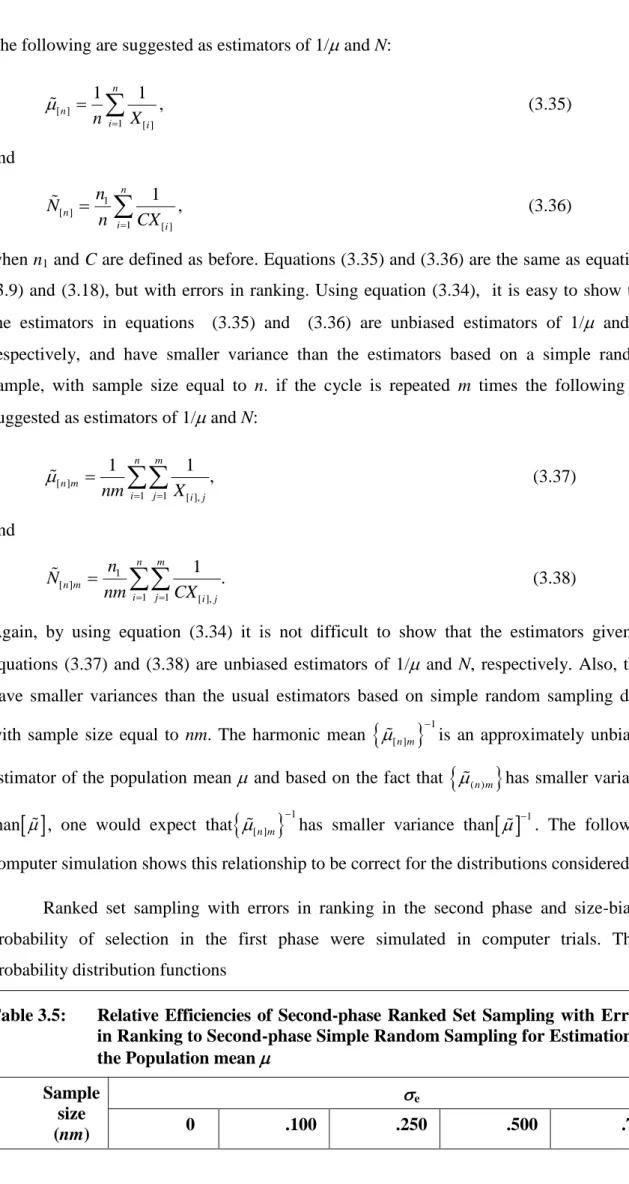
3.2: Estimation of the Population Mean 33
3.3. Estimation of the Population Size N 35
3.4. Computer Simulation Results 37
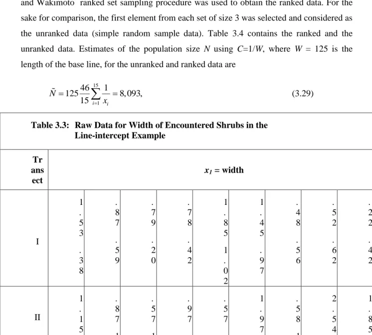
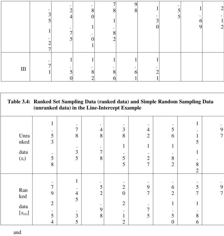
3.5. Numerical Example 39
3.6: Ranked Set Sampling with Probability of Selection Proportional to Size and Errors in Ranking
4
STATISTICAL QUALITY CONTROL BASED ON PAIR AND
SELECTED RANKED SET SAMPLING
45-66
4.1 Introduction 45
4.2 Sampling Methods 51
4.3 Ranked Set Sampling With Concomitant Variable 151 4.4 Quality Control Chart Using Simple Random Sampling (SRS) 54 4.5 Quality Control Charts Using Paired Ranked Set Sampling (PRSS) 55 4.6 Quality Control Charts Using Selected Ranked Set Sampling (SRSS) 57
5
QUALITY CONTROL CHART FOR THE MEAN USING
DOUBLE RANKED SET SAMPLING
67-82
5.1. Introduction 67
5.2. Control Chart Based on Double Ranked Set Sampling (DRSS) 67 5.3: Visual Comparison of DRSS With SRS 68 5.4. Average Run Length Comparison of DRSS 69 5.5. Control Chart Based on MDRSS 71 5.6. Visual Comparison of MDRSS with SRS 71 5.7. Average Run Length Comparison Of MDRSS 72 5.8. Control Chart Based on DMRSS 74 5.9. Visual Comparison of DMRSS With SRS 74 5.10. Average Run Length Comparison of DMRSS 75 5.11. Comparing the New Charts Based on the Standard 3-Sigma 77
5.12. Applications 79
5.13. Construction of Control Charts Using Real Data 80
BASICS OF RANKED
SET SAMPLING
Chapter I
Basics of Ranked Set Sampling
1.1. INTRODUCTION
ne of the keys to any Statistical inference is that the data involved be obtained via some formal mechanism that enables the experimenter to make valid judgments on the question(s) of interest. One of the most common mechanisms for obtaining such data is that of a simple random sample. Other more structured sampling designs, such as stratified sampling or probability sampling, are also available to help make sure that the obtained data collection provides a good representation of the population of interest. Any such additional structure of this type revolves around how the sample data themselves should be collected in order to provide an informative image of the larger population. With any of these approaches, once the sample items have been chosen the desired measurement(s) is collected from each of the selected items.
The most commonly used sampling approach for collecting data from a population with the goal of making inferences about unknown features of the population is that of a simple random sample (SRS). The observations in an SRS are mutually independent if the sampling is from an infinite population or with replacement from a finite population and they are dependent if sampling from a finite population without replacement. In either situation, however, there is a probabilistic guarantee that each measured observation in an SRS can be considered representative of the population. Despite this assurance, there remains a distinct possibility that a specific SRS might not provide a truly representative picture of the population.
With this issue in mind, statisticians have developed a variety of ways to guard against obtaining such unrepresentative samples. Sampling designs such as stratified sampling probability sampling and cluster sampling all provide additional structure on the sampling process to improve the likelihood that the collected sample data provide a good representation of the underlying population. A secondary goal in most data collection settings is to minimize the costs associated with obtaining the data, including both the cost
O
of initially selecting the population units for measurement and in making the actual measurements.
The idea of ranked set sampling was first proposed by Mclntyre(1952) in his effort to find a more efficient method to estimate the yield of pastures. Measuring yield of pasture plots requires moving and weighing the hay which is time-consuming. But an experienced person can rank by eye inspection fairly accurately the yields of a small number of plots without actual measurement. Mclntyre adopted the following sampling scheme. Each time, a random sample of k pasture lots is taken and the lots are ranked by eye inspection with respect to the amount of yield. From the first sample, the lot with rank 1 is taken for cutting and weighing. From the second sample, the lot with rank 2 is taken, and so on. When each of the ranks from 1 to k has an associated lot being taken for cutting and weighing, the cycle repeats over again and again until a total of m cycles are completed. Mclntyre illustrated the gain in efficiency by a computation involving five distributions. He observed that the relative efficiency, defined as the ratio of the variance of the mean of a simple random sample and the variance of the mean of a ranked set sample of the same size, is not much less than (k+1)/2 for symmetric or moderately asymmetric distributions, and that the relative efficiency diminishes with increasing asymmetry of underlying distribution but is always greater than 1. Mclntyre also illustrated the estimation of higher moments. In addition, Mclntyre mentioned the problem of optimal allocation of the measurements among the ranks and problems of ranking error and possible correlation among the units within a set, etc. Though there is no theoretical rigor, the work of Mclntyre is pioneering ad fundamental since the spores of many later developments of RSS.
The idea of ranked set sample seemed buried in the literature for a long time until Halls & Dell (1966) conducted a field trial evaluating its applicability to the estimation of forage yields in a pine hard wood forest. The terminology ranked set sampling was, infact, coined by Halls & Dell. The first theoretical result about RSS was obtained by Takahasi and Wakimoto (1968). They proved that, when ranking is perfect, RSS mean is an unbiased estimator of population mean, and the variance of RSS mean is always smaller than the variance of the mean of a SRS of the same size. Dell & Clutter later obtained similar results, however, without restricting to the case of perfect ranking. Dell & Clutter (1972) and David & Levine (1972) were the first to give some theoretical treatments on imperfect ranking. Stokes (1976, 1977) considered the use concomitant variables in RSS. Up to this point, the attention had been focused mainly on the non-parametric estimation of population mean. A few years later Stokes (1980) considered the estimation of population variance and the estimation of correlation coefficient of a bivariate normal population based on RSS. However, other statistical procedures and new methodologies in the context of RSS had yet to be investigated and developed.
The middle of 1980‟s was a turning point in the development of the theory and methodology of RSS. Since then, various statistical procedures with RSS, non-parametric or parametric, have been investigated, variations of the original notion of RSS have been proposed and developed, and sound general theoretical foundations of RSS have been laid. A few references of these developments are given below. The estimation of cumulative distribution function with various settings of RSS was considered by Stokes and Sager (1988), Kvam and Samaniego (1993) and Chen (2000). The RSS version of distribution-free test procedures such as sign test, signed rank test and Mann-Whitney-Wilconxon test were investigated by Bohn and Wolfe(1992,1994), and Hettmansperger (1995).The estimation of density function and population quantiles using RSS data were studied by Chen (1999, 2000). The RSS counterpart of ratio estimate was considered by Samawi and Muttlak (1996). The U-statistic and M-estimation The U-statistic and M-estimation based on RSS were considered, respectively, by Presnell and Bohn (1999) And Zhao and Chen (2002). The RSS regression estimate was tackled by Patil et al. (1993), Yu Lam (1997) and Chen (2001). The parametric RSS assuming the knowledge of the family of the underlying distribution was studied by many authors, e.g., Abu- Dayyeh and Muttlak (1996), Bhoj (1997) and Ahsanullah (1996), Fei et al. (1994), Li and Chuiv (1997), Shen(1994), Sinha et al. (1996), Stokes (1995), Chen(2000). The optimal design in the context of unbalanced RSS was considered by Stokes (1995), Kaur et al. (1997,), Ozturk and Wolfe (1998), Chen and Bai (2000) and Chen (2001). A general theory on parametric and non-parametric RSS was developed by Bai and Chen (2003). Ranked mechanisms based on the use of multiple concomitant variables were developed by Chen and Shen (2003) and Chen (2002). The Ranked set sampling method is modified to yield new sampling methods. Several modifications for the ranked set sampling were introduced by several authors.
1.2 BALANCED RANKED SET SAMPLING
The goal of RSS is to collect observations from a population that are more likely to span the full range of values in the population (and, therefore, be more representative of it) than the same number of observations obtained via simple random sampling. In its most straightforward and original form, ranked set sampling proceeds as follows. To obtain an RSS of k observations from a population, an initial SRS of k units is selected from the population and rank ordered on the attribute of interest. A variety of mechanisms can be used to obtain this ranking, including visual comparisons, expert opinion, or through the use of auxiliary variables, but it cannot involve actual measurements of the attribute of interest on the sample units. The unit that is judged to be the smallest in this ranking is included as the first item in the RSS and the attribute of interest is formally measured for this unit. This initial measurement is denoted by X[1], where a square bracket is used instead of the usual
the smallest attribute measurement among the k units in the SRS, even though our ranking judged it to be the smallest. The remaining k–1 units (other than X[1] in our initial SRS are
not considered further in making inferences about the population – their role was solely to assist in the selection of the smallest ranked unit for measurement.
Following the selection of X[1], a second independent SRS of size k is selected from
the population and ranked in the same manner as the first SRS. From this second SRS, we select the item ranked as the second smallest of the k units and add its attribute measurement, X[2], to the RSS. From a third independent SRS of size k, we select the unit
ranked to be the third smallest, X[3], for attribute measurement and inclusion in the RSS.
This process continues until we have selected the unit ranked to be the largest of the k units in the kth independent SRS, denoted by X[k], for attribute measurement and inclusion in our
RSS.
This entire process results in the k measured observations X[1], …, X[k] and is called a
cycle. The number of units, k, in each SRS is called the set size. Thus to complete a single ranked set cycle, we need to use a total of k2 units from the population to separately rank k
independent SRSS of size k each. The measured observations X[1], …, X[k] constitute a
balanced ranked set sample of size k, where the descriptor „balanced‟ refers to the fact that
we have collected one judgment order statistic for each of the ranks 1,2,…, k.
To obtain a balanced RSS with a desired total number of measured observations (i.e. sample size) n = km, we repeat the entire process for m independent cycles, yielding the following balanced RSS of size n:
[1]1 [1]2 [1]3 [1] [2]1 [2]2 [2]3 [2] [ ]1 [ ]2 [ ]3 [ ] 1 2 k k k k k k k Cycle X X X X Cycle X X X X Cycle k X X X X
Since its inception with the paper by McIntyre, a good deal of attention has been devoted to the topic and there has been an explosion of interest in and a tremendous amount of methodological development of ranked set sampling procedures particularly over the last few years. Some of this work has been geared toward specific parametric families and some has been developed under minimal non-parametric distributional assumptions. However, many of the important concepts and features of the ranked set sampling methodology transcend the parametric or non-parametric categories
One reason for this increase is the recognition by statisticians of the need for more cost-effective sampling procedures, such as those that use a prior knowledge or can
otherwise provide the needed information with a significant reduction in cost over the more traditional simple random sampling approaches.
The means of Simple Random Sample X and Ranked Set Sample *
X for common measured number of observations is an unbiased estimator of the population mean, , and that it has RSS has variance lesser than SRS.
Of course, there is certainty a difference between these unbiased estimators X and *
X . The k components of the SRS average X are mutually independent and identically distributed and each is itself an unbiased estimator for . While the k components of the RSS *
X are also mutually independent, they are not identically distributed and none of them (except for the middle order statistic when k is odd and the underlying distribution is unbiased for . Yet the average process leaves *
X unbiased. Interestingly, it is the additional structure associated with the non-identical nature of the distribution for the terms in *
X that leads to the improvement in precision for *
X relative to X . In the case of perfect ranking not only is *
X an unbiased estimator, its variance is always no larger than the variance of the SRS estimator X based on the same number of measured observations. In fact, this is a strict inequality unless
*( )i
for all i=1,…,k, which is the case only if the judgment rankings are purely random.1.3. UNBALANCED RANKED SET SAMPLE
There are situations where measuring differing numbers of the various judgment order statistics (unbalanced RSS) can lead to improved RSS procedures. The choice of set size remains important for this unbalanced RSS setting but the concept of a cycle is no longer necessary, since we do not need to have the same measurement counts for every judgment order statistic. Collection of an unbalanced RSS with set size k and total number of measured observations n proceeds as follows. Let n1,…,nk be any positive integers such
that n1+n2+…+nk = n. Collect n independent SRSS, each of size k. Using any appropriate
ranking scheme that does not involve measurement of the variable of interest, rank order the
k observation from least to greatest within each of the n SRSS. Select n1 of these rank
ordered sets of size k at random and measure the smallest judgment order statistic in each of them. From the remaining n–n1, ordered sets of size k, randomly select another n2 ordered
sets and measure the second smallest judgment order statistic in each of them. Continue in this fashion until you measure the largest judgment order statistic in each of the final nk ordered sets.
For each r = 1,…,k, let X[r]j denote the measurement for the rth smallest judgment
is an unbalanced RSS of n measured observations with set size k and ordered replications n1,
n2, …, nk. Just as with balanced RSS, the measured units in an unbalanced RSS are mutually independent, but now the numbers of measured units in each of the ranks are not necessarily equal. Balanced RSS corresponds to the special case where n1=n2=…=nk.
There are a number of factors to consider when deciding whether to use balanced or unbalanced RSS, mostly related to the type of inferences of interest and what is known about the shape of the underlying distribution.
Stokes (1995) and Bhoj (1997) were the first to demonstrate the optimality of unbalanced RSS for estimation of a location parameter within the context of a parametric family and Kaur et al. (1997) obtained corresponding results for skewed distributions. Ozturk and Wolfe (2000 & 2001) extended these findings to non-parametric tests.
When the underlying distribution is unimodal and symmetric, the optimal unbalanced RSS procedures are based solely on set medians, which is precisely the region where it is most difficult to be accurate in our rankings. The second area of concern revolves around the rationale for collecting the data in the first place. If the sole goal of the study is to estimate the population mean for a symmetric and unimodal distribution, then the highly unbalanced RSS based on set medians will work just fine. However, if you later decide that you also want to estimate other features, such as the variance or even the c.d.f, of the underlying distribution, median based unbalanced RSS is generally inferior to balanced RSS.
1.4. RANKED SET SAMPLING WITH UNEQUAL SAMPLES
Bhoj gave ranked set sampling procedure with unequal samples. In the case of ranked set sampling with unequal samples (RSSU), n samples are drawn, where the size of the ith sample is ni, i = 1,2,…, n. The steps in RSSU are the same as in RSS. In both
sampling schemes only n observations out of n2 ranked unit are measure accurately. Hence, the comparison of the estimators based on these schemes will be fair. ni = 2i–1 is taken
when n is even half the sample sizes are smaller than n and the other half are greater than n. In the case of odd n, one sample is of size n, (n–1)/2 samples are greater than n, and the other (n–1)/2 samples are smaller than n.
Let x(ii)ni denote the ith ordered observation from the ith sample of size ni = 2i–1. We
note that, when the sample sizes are equal the subscript of sample size is omitted, as in the case of RSS. Then x(ii)ni, i = 1, 2, …, n, constitute our RSSU, where these n observations are
independently distributed. It is easy to show that
nin2. Kaur, Patil, and Taillie (1997) considered an appropriate unequal allocation of samples for skewed distributions in RSS. However, their unequal allocation is brought in via different values of ri, where ri is thenumber of measurements made corresponding to the ith rank for i = 1,2,…,n. In the case of usual RSS, r1 = r2 = … = rn = r. In the proposed sampling scheme, our sample sizes are
unequal and therefore RSSU is entirely different than the unequal allocation considered in the literature.
1.5. ERRORS IN RANKING
For the case with errors in ranking, it is essential to assure that the erroneous rankings are not related to the process of selecting elements for quantification; otherwise, bias could be injected. Consider a set of n elements, one of which is destined to be quantified. They are ordered by the ranker‟s judgment. For purposes of ranked set sampling, the impact of all errors in ordering the set is expressed simply by the difference between the elements that is placed in the position to be quantified and the element that should have been placed there.
The distribution of X[r] is not the distribution of the rth order statistic, because it
includes the influence of errors in ranking judgment. Suppose ranking judgment is so poor as to give a random ordering of the elements in each set. Then
( )r
foreach r. The estimate is unbiased but RP equals 1. In practice, ranking ability will be between the extremes of a random and perfect ordering of the sets. Thus relative precision will depend upon both the characteristics of the parent population and the impact of errors in ranking judgment. Frequently the differences between the erroneously ranked elements are small and the errors have little effect on the within position variance.
1.6. MEDIAN RANKED SET SAMPLING
Muttlak (1997) proposed Median Ranked Set Sampling (MRSS) method which consists of selecting m random samples each of size m units from the population and rank the units within each sample with respect to the variable of interest. If the sample size m is odd, then from each sample select for measurement the ((m+1)/2)th smallest rank (the median of the sample). If the sample size m is even, then select for measurement the (m/2)th smallest rank from the first m/2 samples, and the ((m+2)/2)th smallest rank from the second
m/2 samples. The cycle can be repeated n times if needed to obtain a sample of size nm.
1.7. PAIR RANKED SET SAMPLING (PRSS)
Hossain and Muttlak (1999) gave Paired Ranked Set Sampling (PRSS) method, two sets of n random elements are required to obtain a sample of size two. At first n elements are selected randomly and ordered, the k-th smallest element of the set is considered for measurement, where 1 kn is pre-determined. Similarly, second set of size n elements is again selected randomly and ordered, and the (n–k+1)th smallest of the set is measured. The
procedure can be repeated r times to obtain a sample of size 2r. Note that in the usual RSS method the sample size is required to be a multiple of n and in the PRSS method it is required to be a multiple of 2 and does not depend on the choice of the set size n.
1.8.
EXTREME RANKED SET SAMPLINGRanked set sampling (RSS) assumed perfect ranking i.e. there will be no errors in ranking the units with respect to the variable of interest. In fact for most practical applications, it is not easy to rank the units without errors in ranking. There will be a loss in efficiency, i.e. RSS will give a larger variance due to the errors in ranking the units. To reduce the errors in ranking in estimating the population mean, the Extreme Ranked Set Sampling (ERSS) procedure was introduced by Muttlak (1999). In the Extreme Ranked Set Sampling (ERSS) procedure, select n random samples of size n units from the population and rank the units within each sample with respect to a variable of interest by visual inspection. If the sample size n is even, select from n/2 samples the smallest unit and from the other n/2 samples the largest unit for actual measurement. If the sample size is odd, select from (n-1)/2 samples the smallest unit, from the other (n -1)/2 the largest unit and from one sample the median of the sample for actual measurement. The cycle may be repeated r times to get nr units. These nr units form the ERSS data.
We can see that the ERSS in practical applications can be performed with less errors in ranking the units since all we have to do is find the largest or the smallest of the sample and measure it. The ERSS method is very easy to apply in the field and will save time in performing the ranking of the units with respect to the variable of interest. In addition, this method will reduce the errors in ranking and hence increase the efficiency of the ERSS when compared to RSS.
1.9. PERCENTILE RANKED SET SAMPLING
In the Percentile Ranked Set Sampling (PRSS) procedure, n random samples of size
n units from the population and rank the units within each sample with respect to a variable of interest. If the sample size is even select for measurement from the first n/2 sample the (p(n+1))th smallest rank and from the second n/2 samples the (q(n+1))th smallest rank, where 0p1 and q=1–p. If the sample size is odd, select from the first (n–1)/2 samples the
(p(n+1)th smallest rank and from the other (n–1)/2 samples the (q(n+1))th smallest rank, and from one sample the median for that sample for actual measurement. The cycle may be repeated r times to get nr units. These nr units form the PRSS data.
1.10. DOUBLE RANKED SET SAMPLING
The Double Ranked Set Sampling (DRSS) procedure can be described as the followings: Identify m3 units from the target population and divide these units randomly into m sets each of size m2. The procedure of ranked set sampling is applied on each m2
units to obtain m ranked set sampling each of size m, then again apply the ranked set sampling procedure on the m ranked set sampling sets obtained in the first stage to obtain a
DRSS of size m (Al-Saleh and Al-Kadiri 2000).
1.11. QUARTILE RANKED SET SAMPLING
In Quartile Ranked Set Sampling method, m units are selected from the population and we rank the units within each sample with respect to a variable of interest. If the sample size is even, select for measurement from the first m/2 samples the (q,(m+1))th smallest the (qu(m+1) the smallest rank. If the sample size is odd, select from the first (m – 1)/2 samples
the (11(m+1)) th smallest rank and for the other (m–1)/2 samples the (qu(m+1)) the smallest
rank, and from one sample the median for that sample for actual measurement.
1.12. DOUBLE QUARTILE RANKED SET SAMPLES
The Double Quartile Ranked Set Sampling (DQRSS) procedure can be described as follows. Select m3 units from the population and divide them into m2 sample each of size m. If the sample size is even, select from the first m2/2 sample the [q1(m+1)]th smallest rank,
from the second m2/2 samples the [q3 (m+1)]th smallest rank. If the sample size is odd,
select from the first m(m–1)/2 samples the [q1(m+1))th smallest rank, the median from the
next m samples and the [q3(m+1)] the smallest rank from the second m(m–1)/2 samples.
This step yield m sets each of size m. Apply the QRSS procedure on the m sets obtained earlier to get a DQRSS sample of size m. The whole cycle may be repeated n times to obtain a sample of size mn from DQRSS.
1.13. SELECTED RANKED SET SAMPLING (SRSS)
Hossain and Muttlak (2001) Considered the situation where, instead of selecting n
random sets of size n elements each as in the RSS, only K < n random set of size n
elements are selected, and instead of measuring the ith smallest order statistic of the ith set,
nithsmallest order statistic of the ith set is considered for measurement. The values of
1, 2,..., k 1 1 2 ... k
n n n n n n n
are required to be determined beforehand, see Hossain and Muttlak (2001).
The procedure of selected ranked set sampling (SRSS) can be described as follows: At first, a set of n > k elements is randomly selected and they are ordered by visual
inspection and the n1-th smallest is selected for measurements. Another set of n elements is
randomly selected and they are ordered and the n2-the smallest element is measured, and the
procedure is continued until the nk-th smallest is measured.
1.14. MOVING EXTREMES RANKED SET SAMPLING
Al-Odat and Al-Saleh (2001) introduced the concept of varied set size RSS, which is coined here as Moving Extremes Ranked Set Sampling (MERSS). They investigated this modification non-parametrically and found that the procedure can be more efficient and applicable than the simple random sampling technique (SRS).
The procedure of MERSS is described as follows:
1. Select m random sample of size 1,2,3,…,m, respectively.
2. Identify the maximum of each set by eye or by some other relatively inexpensive method, without actual measurement of the characteristic of interest.
3. Measure accurately the selected judgment identified maximum. 4. Repeat steps 1, 2, 3 but for minimum
5. Repeat the above steps r time until the desired sample size, n = 2rm is obtained. This sample is called Moving Extremes Ranked Set Sample (MERSS).
Clearly, the procedure of MERSS is easier to use than the usual RSS
1.15. MULTISTAGE RANKED SET SAMPLING
The superiority of using ranked set sampling, for estimating the mean of a population, over simple random sampling, is well established. This technique is useful when visual ordering of a small set of size (m) can be done easily and fairly accurately, but exact measurement of an observation is difficult and expensive. It is noted that for many distributions, an increase in the efficiency of ranked set sampling can be achieved by increasing the set size m. However, in practice, m should be kept very small so that visual ranking errors will not destroy the gain in efficiency.
The MSRSS procedure is described as follows:
1. Randomly selected mr+1 sample units from the target population, where r is the number of stages.
2. Allocate the mr+1 selected units randomly into mr−1 sets, each of size m2.
3. For each set in Step (2), ranked set sampling procedure is applied, to obtain a (judgment) ranked set of size m. This step yields mr−1 (judgment) ranked sets, of size m each.
4. Without doing any actual quantification on these ranked sets, repeat Step (3) on the mr−1 ranked set to obtain mr−2 second stage (judgment) ranked sets, each of size m.
5. The process is continued using Step (3), without doing any actual quantification, until we end up with one rth stage (judgment) ranked set of size
m.
6. Finally, the m identified elements in Step (5) are now quantified for the variable of interest.
1.16. L RANKED SET SAMPLING (LRSS)
A robust RSS procedure is suggested based on the idea of L statistic, which will be referred as L Ranked Set Sampling (LRSS). The main idea of this procedure is to discard the data in the tails of a data set (trimming), or replace data in the tails of a data set with the next most extreme data value (winsorizing). In order to plan LRSS design, n random samples should be selected each of size n, where n is typically small to reduce ranking error. For the sake of convenience it is assumed that the judgment ranking is as good as actual ranking. LRSS has the following steps:
Step 1. Select n random samples each of size n units.
Step 2. Rank the units within each sample with respect to a variable of interest by a visual inspection or any other cost-free method.
Step 3. Select the LRSS coefficient, k = [n, α], such that 0 ≤ α < 0 5, where [x] is the largest integer value less than or equal to x.
Step 4. For each of the first k+ 1 ranked samples, select the unit with rank k + 1 for actual measurement.
Step 5. For each of the last k+ 1 ranked samples, i.e., the (n–k)th to the nth ranked sample, select the unit with rank n–k for actual measurement.
Step 6. For j = k + 2,…, nk1, the unit with rank j in the jth ranked sample is selected for actual measurement.
Step 7. The cycle may be repeated r times to obtain the desired sample size n∗r. Without loss of generality, suppose that the cycle is repeated once, r = 1.
For any sample size, when k = 0, then this procedure leads to the novel
RSS, McIntyre‟s procedure. For a sample of size n with k = (n1)/2, then the selected sample leads to the traditional MRSS, i.e., n equal to 5 or 6 and k = 2. Also, the PRSS could be considered as a special case of this scheme.
1.17. BALANCED GROUP RANKED SET SAMPLING
Jemain, Omari and Ibrahim (2008) proposed the Balanced Groups Ranked Set Samples method (BGRSS) for estimating the population mean with samples of size m=3k
where (k = 1,2,…). It was found that the BGRSS produced unbiased estimators with smaller variance than commonly used simple random sampling for symmetric distribution. The balanced groups of ranked set sampling can be described as follows:
Step 1: Randomly select m=3k(k=1,2,….) sets each of size m from the target population, and rank the units within each set with respect to the variable of interest.
Step 2: Allocate the 3k selected sets randomly into three groups, each of size k sets. Step 3: For each group in step (2), select for measurement the lowest ranked unit
from each set in the first group, and the median unit from each set in the second group, and the largest ranked unit from each set in the third group. By this way we have a measured sample of size m=3k units in one cycle. The Steps 1-3 can be repeated n times to increase the sample size to 3kn out of 9k2n units.
The BGRSS method differs from the usual RSS and ERSS methods. In the usual
RSS we identify and measure the ith smallest ranked unit of the ith sample (i=1,2,…,m).In the case when m is odd, for ERSS we select the smallest ranked unit from the first m1/2 sets and the largest ranked unit from the other m1/2 sets. In the case when m is even we select the smallest ranked unit from the first m/2 sets and the largest ranked unit from the other m/2 sets. But in the BGRSS method, the measured units consist of m/3 minima, m/3 medians and m/3 maxima.
Indeed, the BGRSS method is easy to be applied since we only need to identify and measure the lowest rank units of the first k sets, and the medians of the second k sets and the largest rank units from the last k sets. Here, k is any positive integer. However, for practical purposes, k should be small in order to have a small sample size, so that the ranking is easy and errors in ranking is reduced.
Chapter No:2
Estimation Of The Mean Of The Exponential
Distribution Using Moving Extreme Ranked
ESTIMATION OF THE MEAN OF THE
EXPONENTIAL DISTRIBUTION USING MOVING
EXTREME RANKED SET
SAMPLING (MERSS)
Set Sampling (
ME
RSS)
2.1. INTRODUCTION
isher laid the foundation of the theory of estimation, although much of the attention was directed to approximation measures appropriate to large sample. In the present age of computer sophistication, computational difficulty is no longer a justification for seeking alternative and inefficient estimation procedures particularly when there are only two or three parameters to be estimated. Quite often there are many competing methods of estimation and specific method may be superior to other method.
Fei et al., (1994) used RSSto estimate the parameters of Weibull and extreme value distributions. Lam et. al. (1994) used RSS to estimate two parameter exponential distribution. Al-Saleh and Al-Kadiri (2000) considered Double RSS as a procedure that increases the efficiency of RSS estimates without increasing the set size m. Al-Saleh and Al-Omary (2002) generalized Double RSS to multistage RSS and most recently. Barabesi and El-Sharaawi (2001) considered the efficiency of RSS for parametric estimation in general setting demonstrating that parametric inference is generally more efficient than SRS counterpart procedure essentially, to use the procedure we need to be able to (judgment rank) any pairs of elements.
Exponential distribution is a very important and a widely used distribution in statistics and in the field of life-testing. The lifetimes can often be usefully represented by an exponential random variable. Being a skewed distribution, this distribution doesn‟t benefit much from RSS for small set size Takahasi and Wakimoti, (1968). A random variable X has an exponential distribution if it has the probability density function
1 ; , 0, 0; x f x e x with distribution function
; 1x F x e
for x > 0. The MLE and the modified MLE of the population mean were considered. The efficiencies of the estimators were compared with their SRS counterparts. The information in the moving extreme ranked set sampling (MERSS) was measured through Fisher information number. It was seen that the MERSS is more efficient than SRS in estimating the population mean
and the sample obtained using this procedure carry more information about the parameter than a simple random sample of equivalent size.
2.2. THE MAXIMUM LIKELIHOOD ESTIMATOR (MLE)
For a set size m, let (Xm:m, Xm-1:m-1,…, X1:1, Y1:m, Y1:m-1, Y1:m-2,…, Y11) be MERSS
from
; 1x f x e
. If judgment ranking are accurate then for i = 1,…,m, Xi:i has the same
distribution as the ith order statistics of a simple random sample (SRS) of sixe i from f and
Y1:i has the same distribution as the 1st order statistics of a SRSof size i from f. to get the
MLEof . The likelihood function is
1
1 : : 1: 1: 1;
;
;
1
;
m i i i i i i i i iL
if x
F x
if y
F y
The log likelihood is
* : 1: 1 1 log , log , m m i i i i i L C f x f y
:
1:
1 1 1 log , 1 log 1 , m m i i i i i i F x i F y
where C is a constant. Now,
* : 1: 1 : 1 1: , , ) ) , , m i i m i i i i i i f x f y L f x f y
:
1:
1 :: 1 1: , , 1 1 , 1 , m m i i i i i i i i f x f y i i F x F y
Setting * 0, L we get the likelihood equation
:: :: 1: :: 1: : 1 1 1 1 1 1 1 1 1 1 xi i i i i xi i i i i x y m m m y x i i i e e e i e e e
1: 1: 1 1 1 0 i i y m y i e i e
which simplifies to
: : 2 1: 2 2 2 : 1 1 1 1 0 1 i i x i i m m i i i i i x e y mx m my m i i x e
which can be reduced further to
: : : 1: 1 1 1 0 2 2 1 i i i i x m i i i x i x e x y i y m e
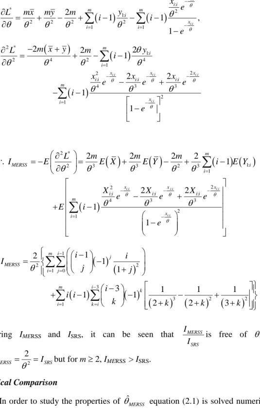
(2.1)Taking the second derivative we have
: 2 *2 : 2 2 2 1 2 1 1 1 2 1 i i x m i i x i x e L m i m e
: : : 1: 3 1 4 1 1 2 2 1 i i i i x m i i i x i x e m x y i y m e
The first term of the above quantity is always negative and the second term is zero at any solution, ˆ, of (2.1). Thus
2 2 ˆ L
< 0. Thus, any solution of (2.1) maximizes the
likelihood and hence (2.1) should have at most one solution. But as 0, LHS of (2.1) goes to a negative number and as it goes to . Hence, (2.1) has a unique solution and this solution is the MLEof . This estimator is denoted by ˆMERSS
2.3. PROPERTIES OF THE ML ESTIMATOR
Theorem 2.1: Assume that the sampling is from an exponential distribution using moving extreme ranked set sampling then for any real number “a”
a) ˆ 1:1 2:2 : 1:1 1: , ,..., m m , ,..., m MERSS X X X Y Y a a a a a
1:1 2:2 : 1:1 1:
1 ˆ , ,..., , ,..., MERSS X X Xm m Y Ym a b) Var ˆMERSS X1:1,X2:2,...,Xm m: ,Y1:1,...,Y1:m a a a a a
1:1 2:2 : 1:1 1:
2 1 ˆ , ,..., , ,..., MERSS m m m Var X X X Y Y a c) The efficiency is free of .
Proof:
a) ˆMERSSis the solution of (2.1)
: : : 1: 1 1 1 0 2 2 1 i i i i x m i i i x i X e X Y i Y m e
(*)Consider 1:1 2:2 : 1:1 1:
, ,..., m m, ,..., m
X X X Y Y
a a a a a . Then the MLE based on these observations is the
solution of
: : : 1: 1 1 1 0 2 2 1 i i i i x i i a m i x i X e Y X Y a i a m a e
i.e.
: : : 1: 1 1 1 0 2 2 1 i i i i x m a i i i x i a X e X Y a i Y m e
(**)Now, if t is a solution of (*) then t
ais a solution of (**). Hence 1:1 2:2 : 1:1 1: ˆ , ,..., m m, ,..., m MERSS X X X Y Y a a a a a
1:1 2:2 : 1:1 1:
1 ˆ , ,..., , ,..., MERSS X X Xm m Y Ym a (b) and (c) follows trivially from (a).
The information number for simple random sample of size 2m from an exponential distribution is ISRS 2m2
.The information number is a MERSSis given in the next theorem.
Theorem 2.2: with 0 1 k for k< i, we have
1 2 2 1 0 1 2 1 1 1 m i j MERSS i j i I i j j
3 3 2 2 1 1 3 1 1 1 1 1 2 2 3 m i k i k i i i k k k k
Proof:The likelihood function:
: : 1 1: 1: 1 1 1 1 . 1 . i i i i i i x x y i y i m i L i e e i e e
: 1: * 1 1 1 1log log log
i i i x y m m i i L L C e e
: 1: 1 1 1 log 1 1 log i i i x y m m i i i e i e
where C is constantNow,
: : : * 2 1: 2 2 2 2 1 1 2 1 1 , 1 i i i i x i i m m i x i i x e y L mx my m i i e
and
2 * 1: 2 4 2 4 1 2 2 2 1 m i i m x y y L m i
: : : : 2 2 : : : 4 3 3 2 1 2 2 1 1 i i i i i i i i x x x i i i i i i m x i x x x e e e i e
2 * 1: 2 3 3 2 3 1 2 2 2 2 1 m MERSS i i L m m m I E E X E Y i E Y
: : : : 2 2 : : : 4 3 3 2 1 2 2 1 1 i i i i i i i i x x x i i i i i i m x i X X X e e e E i e
1 2 2 1 0 1 2 1 1 m i j MERSS i j i i I j j
3 3 2 2 1 3 1 1 1 1 1 2 2 3 m i k i k i i i i k k k k
Comparing IMERSS and ISRS, it can be seen that MERSS
SRS I
I is free of and for
m=1,IMERSS 22 ISRS
but for m 2, IMERSS > ISRS.
Numerical Comparison
In order to study the properties of ˆMERSS equation (2.1) is solved numerically. The simulation confirms the unbiasedness of the estimator. Also, the efficiency of the estimator is compared with that of SRS.
Table 2.1: Summary of a Simulation with 10000 iterations to studyˆMERSSfor Exp (1)
m ˆ
ˆ
MERSS
E Varˆ
ˆMERSS
MSEˆ
ˆMERSS
eff
ˆMERSS,ˆSRS
1 1.00175 0.50104 0.501039 0.9979
2 1.00544 0.20880 0.208833 1.1971
3 1.00853 0.12448 0.124552 1.3381
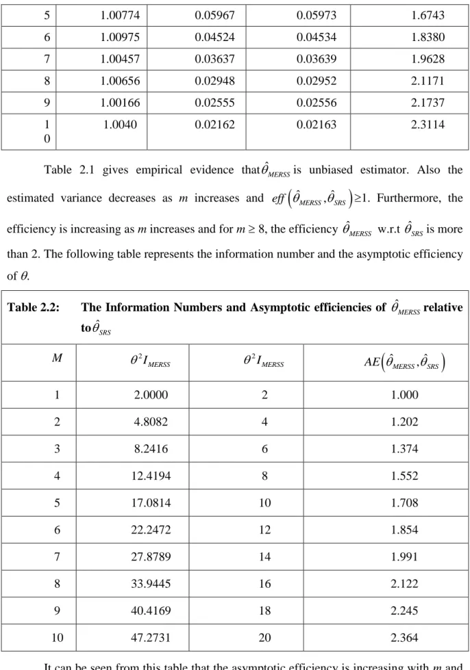
5 1.00774 0.05967 0.05973 1.6743 6 1.00975 0.04524 0.04534 1.8380 7 1.00457 0.03637 0.03639 1.9628 8 1.00656 0.02948 0.02952 2.1171 9 1.00166 0.02555 0.02556 2.1737 1 0 1.0040 0.02162 0.02163 2.3114
Table 2.1 gives empirical evidence that ˆMERSSis unbiased estimator. Also the estimated variance decreases as m increases and eff
ˆMERSS,ˆSRS
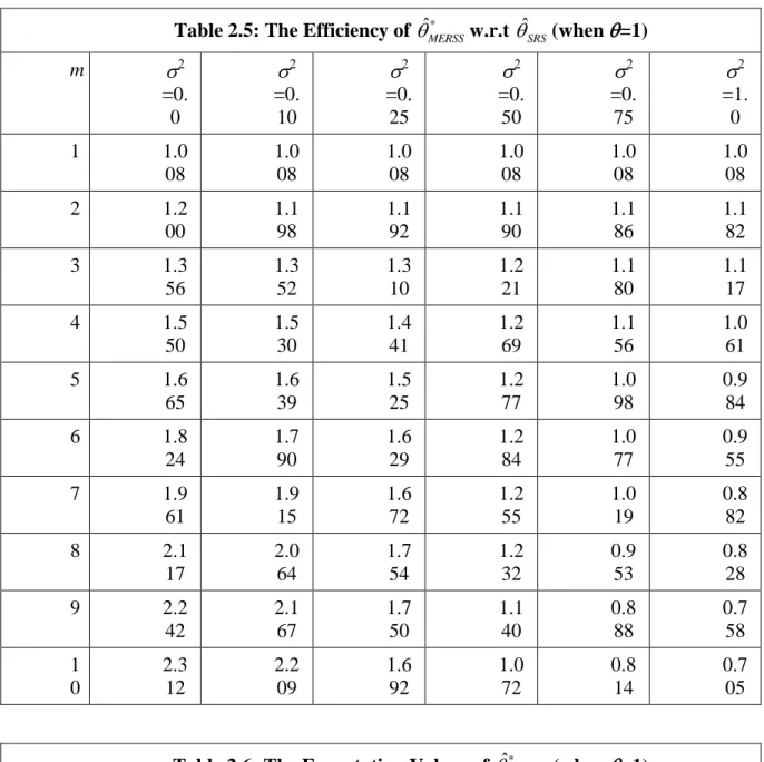
1. Furthermore, the efficiency is increasing as m increases and for m 8, the efficiency ˆMERSS w.r.t ˆSRSis more than 2. The following table represents the information number and the asymptotic efficiency of .Table 2.2: The Information Numbers and Asymptotic efficiencies of ˆMERSSrelative toˆSRS M 2 MERSS I 2 MERSS I
ˆ ,ˆ
MERSS SRS AE 1 2.0000 2 1.000 2 4.8082 4 1.202 3 8.2416 6 1.374 4 12.4194 8 1.552 5 17.0814 10 1.708 6 22.2472 12 1.854 7 27.8789 14 1.991 8 33.9445 16 2.122 9 40.4169 18 2.245 10 47.2731 20 2.364It can be seen from this table that the asymptotic efficiency is increasing with m and is always larger than 1 for m > 1. Note also that the relative efficiencies reported in Table 2.1 are smaller than the corresponding values in Table 2.2, i.e., the reported results of the two tables are in agreement with the Cramer-Rao inequality (information inequality). Furthermore, the two types of efficiency are very close, indicating thatˆMERSS
the Minimum Variance Unbiased Estimator (MVUE), its variance is close to the variance of MVUE (which does not exist).
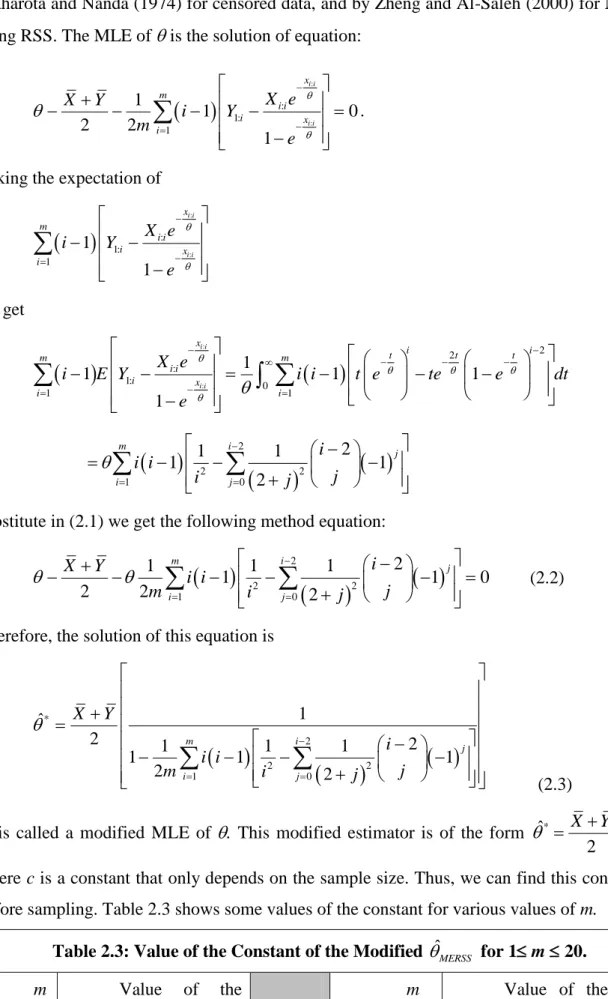
2.4. MODIFIED MLE
In order to get a closed form approximate MLE of , the last term of the left-hand side of the likelihood equation is replaced by its expectation. This technique was used by Maharota and Nanda (1974) for censored data, and by Zheng and Al-Saleh (2000) for MLE using RSS. The MLEof is the solution of equation:
: : : 1: 1 1 1 0 2 2 1 i i i i x m i i i x i X e X Y i Y m e
.Taking the expectation of
: : : 1: 1 1 1 i i i i x m i i i x i X e i Y e
we get
: : 2 2 : 1: 0 1 1 1 1 1 1 1 i i i i x i i t t t m m i i i x i i X e i E Y i i t e te e dt e
2 2 2 1 0 2 1 1 1 1 2 m i j i j i i i j i j
substitute in (2.1) we get the following method equation:
2 2 2 1 0 2 1 1 1 1 1 0 2 2 2 m i j i j i X Y i i j m i j
(2.2)Therefore, the solution of this equation is
* 2 2 2 1 0 1 ˆ 2 1 1 1 2 1 1 1 2 2 m i j i j X Y i i i j m i j
(2.3) * ˆ is called a modified MLE of . This modified estimator is of the form ˆ* * , 2
X Y c
where c is a constant that only depends on the sample size. Thus, we can find this constant before sampling. Table 2.3 shows some values of the constant for various values of m.
Table 2.3: Value of the Constant of the Modified ˆMERSS for 1m 20.
constant constant 1 1.0 11 0.7785 2 1.0 12 0.7632 3 0.9729 13 0.7492 4 0.9412 14 0.7364 5 0.9105 15 0.7245 6 0.8824 16 0.7134 7 0.8570 17 0.7032 8 0.8342 18 0.6936 9 0.8138 19 0.6847 10 0.7953 20 0.6760
From Table 2.3, for m = 1, 2 the constant is exactly 1 and thus ˆ* 2
X Y is
. For m > 2, c is smaller than 1, which means that this constant is a shrinkage factor, i.e. ˆ*
2
X Y
.
Also, for small value of m, ˆ* is not very far from 2
X Y
but the constant gets smaller as m
increases and therefore the estimator departures from 2
X Y
.
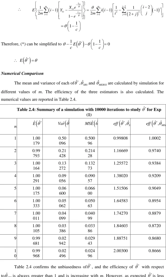
Theorem 2.3: The modified MLE, ˆ*is an unbiased estimator of .
Proof: * ˆ * 2 X Y c
ˆ* * 2 X Y E E c i.e. 1
ˆ* 2 X Y E E c It is well known that under some regularly conditions f x
; dx 0
. As aconsequence of this fact we have: