Prediction of sand production onset in petroleum reservoirs using a reliable classification approach

Original article

Prediction of sand production onset in petroleum reservoirs

using a reliable classi

fi

cation approach

Farhad Gharagheizi

a

, Amir H. Mohammadi

b,c,d,*

, Milad Arabloo

e

, Amin Shokrollahi

e a_{Department of Chemical Engineering, Texas Tech University, Lubbock, TX, United States}

b_{Thermodynamics Research Unit, School of Engineering, University of KwaZulu-Natal, Howard College Campus, King George V Avenue, Durban, 4041,}

South Africa

c_{Institut de Recherche en Genie Chimique et Petrolier (IRGCP), Paris Cedex, France}

d_{Departement de Genie des Mines, de la Metallurgie et des Materiaux, Facult e des Sciences et de Genie, Universite Laval, Quebec (QC), G1V 0A6,}

Canada

e_{Young Researchers and Elites Club, North Tehran Branch, Islamic Azad University, Tehran, Iran}

a r t i c l e i n f o

Article history:

Received 11 October 2015 Received in revised form 31 January 2016 Accepted 3 February 2016 Keywords: Sand production Least square SVM ROC graph

Classification description Modeling

Sanding onset

a b s t r a c t

Controlling sand production in the petroleum industry has been a long-standing problem for more than 70 years. To provide technical support for sand control strategy, it is necessary to predict the conditions at which sanding occurs. To this end, for thefirst time, least square support machine (LSSVM) classification approach, as a novel technique, is applied to identify the conditions under which sand production occurs. The model presented in this communication takes into account different parameters that may play a role in sanding. The performance of proposed LSSVM model is examined usingfield data reported in open literature.

It is shown that the developed model can accurately predict the sand production in a realfield. The results of this study indicates that implementation of LSSVM modeling can effectively help completion designers to make an on time sand control plan with least deterioration of production. Copyright©2016, Southwest Petroleum University. Production and hosting by Elsevier B.V. on behalf of KeAi Communications Co., Ltd. This is an open access article under the CC BY-NC-ND license (http://creativecommons.org/licenses/by-nc-nd/4.0/).

1. Introduction

The sand production prediction is one of the long-standing

and complex problems in the petroleum industry[1]. From the

phenomenological viewpoint, sand production can occur when

the formation do not present sufficient strength to withstand

destabilizing forces generated during theflow of reservoirfluid

[2e4]. A wide variety of problems such as production loss due

to plugging the perforations[2,3,5,6], wellbore instability[6e8],

equipment erosion[2,8e11], and additional costs for waste sand

depositional [8,9,11] can occur due to sand production. This

may result in reduced production time and increased main-tenance and operating costs. It is a complex phenomenon which depends on various factors such as lithology of the formation, stress distribution around the wellbore, reservoir

characteristics (i.e., rock and fluid properties), wellbore/

completion geometry, and production conditions. Due to the importance of sand production prediction in the petroleum industry, great efforts have been directed to develop robust and reliable methods for sand production prediction. Morita

et al.[12]proposed an analytical approach to study the effects

of many parameters on sand production. According to their research following parameters may affect sand production: wellbore pressure and stress distribution around well; drag

forces induced byfluidflow; rock strength of formation; shot

density and perforation geometry; cyclic loading history.

Morita and Boyd [13]presented analyses offive typical sand

problems commonly observed in thefield. Thefirst is the

sear-type sand problem in poorly consolidated sand formation in *Corresponding author. Thermodynamics Research Unit, School of

Engi-neering, University of KwaZulu-Natal, Howard College Campus, King George V Avenue, Durban, 4041, South Africa.

E-mail addresses: a.h.m@irgcp.fr, amir_h_mohammadi@yahoo.com (A.H. Mohammadi).

Peer review under responsibility of Southwest Petroleum University.

Production and Hosting by Elsevier on behalf of KeAi

Contents lists available atScienceDirect

Petroleum

j o u r n a l h o m e p a g e : w w w . k e a i p u b l i s h i n g . c o m / e n / jo u r n a l s/ p e t l m

http://dx.doi.org/10.1016/j.petlm.2016.02.001

2405-6561/Copyright©2016, Southwest Petroleum University. Production and hosting by Elsevier B.V. on behalf of KeAi Communications Co., Ltd. This is an open access article under the CC BY-NC-ND license (http://creativecommons.org/licenses/by-nc-nd/4.0/).

Alaska. The second is the sands produced from intermediate strength formation following water break through. Loss of capillary pressure holding the sand species together is the

pri-mary cause of this sand production[13]. The third is from North

Sea reservoirs where sand was produced from consolidated for-mations with reservoir pressure depletion. The fourth type of sand observed in consolidated formations located in California close to the San Andrea fault with high horizontal tectonic forces.

Finally, thefifth sand production type was produced with high

pressure gradient around cavity surface due to multiple

perfo-rations with high perforation depth. Doan et al.[14]developed

numerical modeling of gravitational deposition of sand in a horizontal well in heavy oil reservoirs. Examination of simulation

results revealed that oil viscosity and_flow rate along with sand

particle size play important roles in the gravity deposition of sands inside horizontal heavy oil reservoirs. Bianco and Halleck

[9] experimentally evaluated the behavior, morphology, and

stability of sand arches near the wellbore in two-phase saturated

sand samples. They analyzed the effects of changes influidflow

velocity and water saturation during the sand production

pro-cess. With the growing use of artificial intelligence modeling in

petroleum engineering, Kanj and Abousleiman[15]developed an

artificial neural network (ANN) modeling to predict important

sanding indication parameters for gas wells of Northern Adriatic Basin. Later, another ANN model was developed by Azad et al.

[16] to predict critical bottom holeflowing pressure inhibiting

sand production using 38 datasets collected from three different

oilfields wells located in the southeast of Iran. The results

showed that the developed model provides better prediction than other analytical models. Although the ANN-based models have been generally proven to provide high accuracy for

pre-diction problems[17e20], they often have some limitations and

shortcomings. They may have the disadvantages of non-reproducibility of results, over-fitting problems, getting stuck in local minima, setting too many controlling parameters, and etc

[21e25]. In this communication, for the first time, a new

computer-based algorithm namely least square support vector machine (LSSVM) modeling approach is presented for identifying the sanding condition.

2. Field data and model development

2.1. Database collection

A data set of 31 wells of Northern Adriatic Basin reported by

Moricca et al. [10] was used for modeling. Adriatic Sea is

geographically bounded by Italy, Albania, and the former Yugo-slavian republics. The northern and central portions of this area are known to form one geological unit commonly referred to as

the Northern Adriatic Basin[10]. The Northern Adriatic Basin is

considered Italy's main supplier in natural gas. Based on exten-sive experimental tests on core samples as well as drilled

cut-tings in different fields of the Northern Adriatic Basin, the

following data were obtained[10]:

1. The producing formation porosity varies between 10 and 40% while it has very low permeability ranging from 10 to 100 mD. 2. The lithology of vertical column is composed of sand shale alterations. While the producing formation contains

unce-mented clays. The cohesive strength averages to 19 kg/cm2.

According to AGIP's research group[10], out of all studied

wells, 23 wells considered as problematic due to sand produc-tion, and the remaining 8 wells considered as sand free. Reported main factors affecting sand production were: total vertical depth

(TVD), transmit time (TT), cohesive strength of the formation (COH), water and gasflow rates (Qw&Qg), bottom holeflowing

pressure (BHFP), drawdown pressure (DD), effective overburden stress (EOVS), shut per foot (SPF), perforation interval (Hperf).

This dataset was examined for incomplete data and as the result

two sets were removed. Thefinalized data set consisting of 29

data points is reported inTable 1.

As previously mentioned, our objective is to develop a math-ematical non-linear relationship between the available data which considered as inputs (i.e., TVD, TT, COH, Qw, Qg, BHFP, DD, EOVS,

SPF, and Hperf) and the output which is sanding indication. For this

purpose, mathematical background of LSSVM is presented.

2.2. Model development

The aim of this section is a review on some basic concept on support vector machines (SVM) for classification problems. SVM

can be considered as a non-probabilistic binary linear classi_fier

using regression analysis. This algorithm that is supervised learning manner for pattern recognition and data analysis has

been studied extensively for both classi_fication and regression

analysis[1,26e34]. The convergence of SVM method to global

optimum and detect a quick solution by standard algorithm is very probable It has no need for multiple adjustable parameters and network topology determination in advance (it will be determined automatically at the end of training process)

[35e38].

The SVM algorithm builds a separating hyper-surface in the input space. This process is performed as follows[1,35,38e40]: 1) It maps the input patterns into a higher dimensional feature

space through nonlinear mapping.

2) Builds a separating hyper-plane with maximum margin. By considering a training sample set of N data points

fxk;ykgNk¼1, in whichxk2Rnis thekth input pattern andyk2Rnis

thekth output pattern, the SVM algorithm is reduced to

con-structing a classifier of the below form for classification

problems: yðxÞ ¼sign " XN k¼1 a_ky_kJðx;x_kÞ þb # (1)

where

ak

positive real constants and b is a real constant.

J

(.,.) is a function that has some forms such as linear SVM, polynomial SVM, two layer neural SVM, and Radial Basis Function (RBF) SVM. Recent studies show that RBF SVM is hemmore reliable that other form of SVM[33,41e43].

The RBF for of this function is as follow:

Jðx;x_kÞ ¼exp ( kxxkk22 s2 ) (2)

where

s

2is the squared variance of the Gaussian function which

should be optimized by the user to obtain the support vector. Construction of classifier based on SVM approach is as follow. One assumes that

yk h

wT4ðxkÞ þb i

1 k¼1; ::::;N (3)

4(.) is a nonlinear function which maps the input space into a

higher dimensional space. The extension of linear SVMs to

Basically it is done by introducing additional slack variables into Eq.(3)as follows:

y_khwT4ðx_kÞ þbi1z_k; k¼1;2; :::;N (4)

z_k0 for k¼1; :::;N

The generalized optimal separating hyperplane is determined

by the vectorw, that minimizes the functional,

minjðw;zÞ ¼1 2w T_wþC 2 XN k¼1 z_k (5) subject to the constraints:

yk h

wT4ðxkÞ þb i

1z_k; k¼1;2; :::;N (6)

whereCis a positive real constant that determines the tradeoff

between the maximum margin and the minimum classification

error[34,38]. In the conventional SVM, optimal separating

hy-perplane is obtained by solving the above quadratic program-ming problem. The solution to the optimization problem of Eq.

(5)under the constraints of Eq.(6)is given by the saddle point

of the Lagrangian[44], Lðw;b;a;z;bÞ ¼1 2w T_wþC 2 XN i¼1 z_iXN k¼1 a_k yk h wT4ðxkÞ þb i 1þz_kXN k¼1 b_kz_k (7)

where

a

and,

b

are the Lagrange multipliers.

2.3. Least Square Supported Vector Machine (LSSVM)

In order to reduce the model complexity of SVM and also to

improve the speed of SVM, a modified version, called least square

LSSVM was proposed by Suykens&Vandewalle[38].

In LSSVM algorithm, solution is obtained by solving a linear set of equations, instead of solving a quadratic programming

problem involved by standard SVM[38].

In contrast to SVM, the LSSVM is trained by minimizing the cost function which is defined as follow[38]:

minjðw;zÞ ¼1 2w t_wþC 2 XN k¼1 z2 k (8)

subject to the constraints[38]:

y_khwT4ðx_kÞ þbi¼1z_k; k¼1;2; :::;N (9) In the LS-SVM, one works with equality instead of inequality constraints. Therefore, the optimal solution can be obtained by solving a set of linear equations instead of solving a quadratic

programming problem [38]. To derive the dual problem for

LSSVM non-linear classification problem, the Lagrange function

is defined as: Lðw;b;z;aÞ ¼1 2w T_wþC 2 XN k¼1 z2 k XN k¼1 a_k nðyk h wT4ðxkÞ þb i 1þz_kÞo (10)

where

ak

values are Lagrange multipliers, which is positive or

negative due to LSSVM formulation. The conditions for optimally are derived by differentiating the above equation with respect to Table 1

Field data[10]and predicticted results of proposed LSSVM model.

No. TVD TT COH Qg Qw BHFP DD EOVS SPF Hperf Field observed LSSVM predicted

1 319 105 22 42.3 5672 133.2 27.8 651 4 14 1a ₁ 2 3182 105 21.9 51.2 68 140.4 16.6 642 4 16 1 1 3 3366 100 24.7 66.9 157 156.2 18.9 601 4 6 1 1 4 3647 100 29.6 80.6 85 153.8 57.8 670 8 20 1 1 5 4548 85 53.2 48 886 209.1 58.9 823 4 18 1 1 6 4088 85 39.5 72.7 116 147 44 781 2 17 1 1 7 2100 115 10.8 28.5 724 160.1 8.9 300 4 15.5 1 1 8 1930 132 9.7 27.5 695 175.5 11.2 245 4 11.5 1 1 9 2139 112 11.1 36.8 280 185.5 6.1 283 4 10.5 1 1 10 2380 110 13 23 42 113 47.4 413 6 11 1 1 11 1122 150 5.7 108 0 107 8 115 12 10.5 1 1 12 1340 130 6.6 51 52 126.6 14.4 140 12 6.5 1 1 13 1070 170 5.5 82 70 103.8 0.7 111 4 9 1 1 14 1920 130 9.6 111 0 248 82 153 4 9 1 1 15 2530 100 14.3 58 68 302.2 97.8 242 4 4.5 1 1 16 1640 145 8 94 1260 189 46.8 150 12 10 1 1 17 2130 120 11 86 112 268.3 31.7 179 4 3.5 1 1 18 3655 100 19.8 69.8 1780 287.6 9.1 553 4 21 1 1 19 3668 100 30 75.8 150 272.3 9.2 571 4 21 1 1 20 1503 125 7.3 139.5 35 152.3 2.2 177 4 11.5 1 1 21 3170 100 21.7 48 2823 222.1 6.4 485 4 16 1 1 22 3197 95 22.1 73 273 184.6 48.6 535 2 12 1b ₁ 23 3230 105 22.6 117 68 210 10 517 27 4 1 1 24 3684 95 30.3 108.7 36 266.6 59.7 581 1 12 1 1 25 3005 93 19.5 55 91 67 1 615 33 4 1 1 26 3790 85 32.5 93.4 77 217.2 124.4 654 8.5 12 1 1 27 2750 98 16.5 125.8 75 251.8 3 372 8.5 4 1 1 28 2983 98 19.2 48 28 102 6.1 581 12 4 1 1 29 3175 100 21.8 30.3 1.698 216.1 17.1 492 20 4 1 1

a_{Sand production was observed.} b _{Sand production was not observed.}

w,

zk

,b, and

ak

, and then equating the resulting equations to zero (Eq.(11)). 8 > > > > > > > > > > > > > > > > < > > > > > > > > > > > > > > > > : vL vw¼00w¼ XN k¼1 a_kyk4ðxkÞ vL vb¼00 XN k¼1 a_kyk¼0 vL vz_k¼00ak¼Czk k¼1; ::::;N vL va_k¼00yk h wT_4ðx kÞ þb i 1þz_k¼0 k¼1; ::::;N (11)

The optimality condition (Eq.(11)) can be written as follow

[45]: 2 6 6 4 I 0 0 ZT 0 0 0 YT 0 0 CI I Z Y I 0 3 7 7 5 2 6 6 4 w b z a 3 7 7 5¼ 2 6 6 4 0 0 0 l ! 3 7 7 5 (12) where Z¼ ½4ðx1ÞT_y 1;:::::::::::::;4ðxNÞTyN, Y¼ ½y1; ::::::::::;yN, l ! ¼ ½l; ::::::::::;l,z¼ ½z1; ::::::::::;zN,a¼ ½a1; ::::::::::;aN. The solution is as follow:

0 YT Y ZZTþC1I b a ¼ 0 I (13)

By applying Mercer's condition to the matrix (

U

¼ZZT), we

have:

Ukl¼ykyl4ðxkÞT4ðxlÞ ¼ykylJðxk;xlÞ (14) Hence, the classifier (Eq.(1)) is found by solving the linear set

of Eq.(13)e(14)instead of quadratic programming. The detailed

information can be found in papers presented by Suykens and

Vandewalle[38].

3. Results and discussion

In order to develop the LSSVM classification model, the

MATLAB programming workspace was used. Initially, the dataset was divided into“training”and“validating”sets. The optimum values of the parameters of LSSVM algorithm namely

s

2 _and

_g

_{were evaluated by simulated annealing (SA) [46].}

Determined optimized values are:

s

2¼444.420282248436 and

g

¼ 10475.3147940118. It is worth it to point out that the

numbers of the reported digits of these parameters are gener-ally determined by sensitivity analysis of the total errors of the optimization procedure with respect to the corresponding values.

The most common method for evaluation of the quality of a

classification model is to compute a confusion matrix of the

actual class versus predicted class[47]. From this matrix some

parameters including true positives (TP), true negatives (TN), false positives (FP) and false negatives (FN) can be extracted and used to evaluate a binary classification model. In order to validate

the classification model, the Receiver Operating Characteristic

(ROC) curve can be used to measure the performance of a clas-sifier[48e51]. It is useful for assessing the accuracy of a binary classification.

ROC utilizes some parameters namely, goodness-of-fit,

robustness and predictivity of the classification. Goodness offit was estimated based on the accuracy (ACC), sensitivity (SE) and

speci_ficity (SP). Accuracy (AC) is the simplest type of LSSVM

quality measures and represents the ratio of the correctly assigned cases. Sensitivity (SE) is the rate at which model correctly classifies an observed sanding as observed. Specificity (SP) is the fraction of the correct classified cases from all of the population. ACC, SE, and SP are calculated in the following way, respectively: ACC¼ TPþTN TPþFNþTNþFP (15) SE¼ TP TPþFN (16) SP¼ TN TNþFP (17)

where, FP (false positive) is the number of errors made by

pre-dicting a case being “sanding” while field observation is “no

sanding”and FN (false negative) is the number of errors made by

predicting a case being“no sanding”whilefield observation is

“sanding”. TP and TN refer to the number of true positive and

true negative, respectively. Mattew's[52]correlation coefficient (MCC) is another statistic was also used for measuring the quality

of proposed classi_fication model. MCC is calculated by the

following equation:

MCC¼ ffiffiffiffiffiffiffiffiffiffiffiffiffiffiffiffiffiffiffiffiffiffiffiffiffiffiffiffiffiffiffiffiffiffiffiffiffiffiffiffiffiffiffiffiffiffiffiffiffiffiffiffiffiffiffiffiffiffiffiffiffiffiffiffiffiffiffiffiffiffiffiffiffiffiffiffiffiffiffiffiffiffiffiðTPTNÞ ðFPFNÞ ðTPþFPÞðTPþFNÞðTNþFPÞðTNþFNÞ

p (18)

The values of MCC vary between1 andþ1, whereþ1

rep-resents a perfect prediction, 0 an average random prediction,

and1 an inverse prediction[52]. Thefinal performance of the

proposed model was determined by measuring the ACC, SE, SP and MCC for both training and test sets.

The proposed LSSVM classification parameters are reported in

Table 2. As shown in this table the obtained values for FP, FN, SE, SP, ACC, and MCC for both_“training_”and_“test_” sets are exact.

This similarity indicates that the over-fitting has not been

occurred during the training phase. Also as shown inTable 1

none of cases in original_field data set was misclassi_fied. It is

worth noting that the criterion for onset of sand production is observation of little amount of sand during production or a spoonful as mentioned in the literature.

In addition to these statistical parameters, performance of the

developed LSSVM classifier was evaluated by ROC curve. As it was

previously mentioned, it is used for assessing the separation

ability of a binary classifier[48]. The ROC curve can be

repre-sented by plotting the fraction of TP (or sensitivity) versus the fraction of FP (or 1-specificity). In order to plot the ROC curve, the optimal operating point of the ROC curve, namely, TP and FP should be initially calculated. The slope of ROC curve is defined as: S¼costðP«NÞ costðN«NÞ

costðN«PÞ costðP«PÞ N

P (19)

where costðA«BÞis the cost of assigning an instance of class A to class B. P (total instance of positive class) and N (total instance of

Table 2

Statistical classification parameters obtained for proposed LSSVM model. TP TN FP FN SE SP ACC MCC Training set 19 5 0 0 1 1 1 1

negative class) are TPþFN and TNþFP, respectively. It should be mentioned that costðP«NÞ, costðN«NÞ, costðN«PÞand costðP«PÞ

are calculated from confusion matrix as follows: TP FN FP TN ¼ costðP«PÞ costðN«PÞ costðP«NÞ costðN«NÞ (20) The ROC curve should be plotted by moving the straight line

with slope S from upper left corner of the ROC plot (FP¼0,

TP¼1) down and to the right until it intersects the ROC curve.

An ROC curve is a two-dimensional depiction of classifier

performance. The area under the ROC curve is an index of

goodness of the classification model and has an important

sta-tistical property[49]. It is equivalent to the Wilcoxon test of

ranks[51]and closely related to the Gini coefficient[47]which is

twice the area between the diagonal and the ROC curve[49]. For

a perfect classifier model, the area under curve would be 1, and if

the area equals 0.5, the classifier model has no discriminative

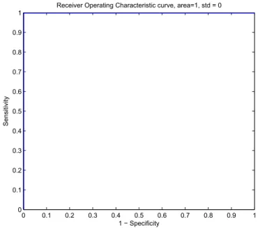
power at all. The ROC curves for both training and test sets are given inFigs. 1 and 2, respectively. The area under the ROC curve was 1 for both training and test sets, stating once again the high predictive power of our developed model.

To make a judgment based onTables 1 and 2andFigs. 1e2, it is concluded that developed LSSVM model is a very promising tool for sand production prediction. Thus, implementation of LSSVM modeling can effectively help completion designers to make an on time sand control plan with minimum impairment of production.

4. Conclusions

To provide technical support for sand control decision-making, it is necessary to identify the conditions at which sanding occurs. For this purpose, a novel compute-based model based on LSSVM methodology was developed for improved prediction of conditions under which sand is produced. A total of

29field data set was employed to construct and test the model.

Results of statistical quality measures and ROC graphs showed

that the proposed model has high classification power in

iden-tifying the sanding conditions. The results of present study will facilitate the strategies for sand-control decision making.

List of symbols

AC accuracy

B bias term

BHFP bottom holeflowing pressure (Kg/cm2)

C a positive constant

COH cohesive strength of the formation (Kg/cm2)

DD drawdown pressure (Kg/cm2₎

ek regression error

EOVS effective overburden stress (Kg/cm2)

FP false positives

FN false negatives

Hperf thickness of perforation interval (meter)

K(x,xk) Kernel function

LSSVM least-squares supported vector machine

MCC Mattew's correlation coefficient

MSE mean square error

Qg gas production rate (K standard m3/day)

Qw water production rate (liter/day)

RBF radial basis function

ROC receiver operating characteristic

SE sensitivity

SP specificity

SPF shot per foot

T transpose

TN true negatives

TP true positives

TT transmit time (micro second/ft)

TVD true vertical depth (meter)

Yrep:=predirepresented/predicted output of the model Greek letters

w a nonlinear function

ai

Lagrange multipliers

g

relative weight of the summation of the regression

errors

s

2 _{squared bandwidth} 0 0.1 0.2 0.3 0.4 0.5 0.6 0.7 0.8 0.9 1 0 0.1 0.2 0.3 0.4 0.5 0.6 0.7 0.8 0.9

1 Receiver Operating Characteristic curve, area=1, std = 0

1 − Specificity

Sensitivity

Fig. 1.Receiver operating characteristic (ROC) curve of the developed LSSVM model built on the basis of the training data.

0 0.1 0.2 0.3 0.4 0.5 0.6 0.7 0.8 0.9 1 0 0.1 0.2 0.3 0.4 0.5 0.6 0.7 0.8 0.9

1 Receiver Operating Characteristic curve, area=1, std = 0

1 − Specificity

Sensitivity

Fig. 2.Receiver operating characteristic (ROC) curve of the developed LSSVM model built on the basis of the test data.

References

[1] S.R. Amendolia, et al., A comparative study of K-nearest neighbour, support vector machine and multi-layer perceptron for thalassemia screening, Chemom. Intell. Lab. Syst. 69 (1e2) (2003) 13e20.

[2] HARV, et al., The diagnosis, well damage evaluation and critical drawdown calculations of sand production problems in the Ceuta Field, Lake Mar-acaibo, Venezuela, in: Latin American and Caribbean Petroleum Engi-neering Conference, Caracas, Venezuela, 1999.

[3] H. Rahmati, et al., Review of sand production prediction models, J. Petrol. Eng. 2013 (2013) 16.

[4] G. Servant, P. Marchina, J.-F. Nauroy, Near-wellbore modeling: sand pro-duction issues, in: SPE Annual Technical Conference and Exhibition, Ana-heim, California, U.S.A, 2007.

[5] D. Tiab, S.A. Rbeawi, The impact of sand and asphaltic production problems on pressure behavior andflow regimes, in: 2012 SPE Kuwait International Petroleum Conference and Exhibition, Kuwait City, Kuwait, 2012. [6] S.M. Willson, Z.A. Moschovidis, J.R. Cameron, I.D. Palmer, New model for

predicting the rate of sand production, in: SPE/ISRM Rock Mechanics Conference, Irving, Texas, 2002.

[7] J. Wang, A. Settari, D. Walters, R. Wan, An Integrated Modular Approach to Modeling Sand Production and Cavity Growth with Emphasis on the Multiphase and 3D Effects, 41st U.S. Symposium on Rock Mechanics, American Rock Mechanics Association, Colorado, 2006.

[8] L. Zhang, M.B. Dusseault, Sand-production simulation in heavy-oil reser-voirs, SPE Reserv. Eval. Eng. 7 (6) (2004) 399e407.

[9] L.C.B. Bianco, P.M. Halleck, Mechanisms of arch instability and sand pro-duction in two-phase saturated poorly consolidated sandstones, in: SPE European Formation Damage Conference, the Hague, Netherlands, 2001. [10] G. Moricca, G. Ripa, F. Sanfilippo, F.J. Santarelli, Basin Scale Rock Mechanics:

Field Observations of Sand Production, Rock Mechanics in Petroleum En-gineering, Delft, Netherlands, 1994.

[11] F. Sanfilippo, G. Ripa, M. Brignoli, F.J. Santarelli, Economical management of sand production by a methodology validated on an extensive database of

field data, in: SPE Annual Technical Conference and Exhibition, Dallas, Texas, 1995.

[12] N. Morita, D. Whitfill, O. Fedde, T. Levik, Parametric study of sand-production prediction: analytical approach, SPE Prod. Eng. 4 (1) (1989) 25e33. [13] N. Morita, P.A. Boyd, Typical sand production problems case studies and

strategies for sand control, in: SPE Annual Technical Conference and Exhibition, Dallas, Texas, 1991.

[14] Q.T. Doan, L.T. Doan, S.M.F. Ali, M. Oguztoreli, Sand deposition inside a hor-izontal well-a simulation approach, J. Can. Petrol. Technol. 39 (10) (2000). [15] M. Kanj, Y. Abousleiman, Realistic sanding predictions: a neural approach,

in: SPE Annual Technical Conference and Exhibition, Houston, Texas, 1999. [16] M. Azad, G. Zargar, R. Arabjamaloei, A. Hamzei, M. Ekramzadeh, A new approach to sand production onset prediction using artificial neural net-works, Petrol. Sci. Technol. 29 (19) (2011) 1975e1983.

[17] A. Chamkalani, et al., Soft computing method for prediction of CO2 corrosion inflow lines based on neural network approach, Chem. Eng. Commun. 200 (6) (2013) 731e747.

[18] A. Chapoy, A.-H. Mohammadi, D. Richon, Predicting the hydrate stability zones of natural gases using artificial neural networks, Oil Gas Sci. Technol. Revue de l'IFP 62 (5) (2007) 701e706.

[19] R. Gharbi, A. Elsharkawy, Neural network model for estimating the PVT properties of Middle East crude oils, SPE Reserv. Eval. Eng. 2 (3) (1999) 255e265.

[20] S.M.J. Majidi, A. Shokrollahi, M. Arabloo, R. Mahdikhani-Soleymanloo, M. Masihi, Evolving an accurate model based on machine learning approach for prediction of dew-point pressure in gas condensate reser-voirs, Chem. Eng. Res. Des. 92 (5) (2014) 891e902.

[21] M. Arabloo, M.-A. Amooie, A. Hemmati-Sarapardeh, M.-H. Ghazanfari, A.H. Mohammadi, Application of constrained multi-variable search methods for prediction of PVT properties of crude oil systems, Fluid Phase Equilibr. 363 (2014) 121e130.

[22] K.-S. Shin, T.S. Lee, H.-j. Kim, An application of support vector machines in bankruptcy prediction model, Expert Syst. Appl. 28 (1) (2005) 127e135. [23] S.R. Taghanaki, et al., Implementation of SVM framework to estimate PVT

properties of reservoir oil, Fluid Phase Equilibr. 346 (2013) 25e32. [24] F.E.H. Tay, L. Cao, Application of support vector machines infinancial time

series forecasting, Omega 29 (4) (2001) 309e317.

[25] B. Verlinden, J.R. Duflou, P. Collin, D. Cattrysse, Cost estimation for sheet metal parts using multiple regression and artificial neural networks: a case study, Int. J. Prod. Econ. 111 (2) (2008) 484e492.

[26] A. Baylar, D. Hanbay, M. Batan, Application of least square support vector machines in the prediction of aeration performance of plunging overfall jets from weirs, Expert Syst. Appl. 36 (4) (2009) 8368e8374.

[27] T.-S. Chen, et al., A novel knowledge protection technique base on support vector machine model for anti-classification, in: M. Zhu (Ed.), Electrical Engineering and Control. Lecture Notes in Electrical Engineering, Springer Berlin Heidelberg, 2011, pp. 517e524.

[28] A. Fayazi, M. Arabloo, A.H. Mohammadi, Efficient estimation of natural gas compressibility factor using a rigorous method, J. Nat. Gas Sci. Eng. 16 (2014) 8e17.

[29] A. Fayazi, M. Arabloo, A. Shokrollahi, M.H. Zargari, M.H. Ghazanfari, State-of-the-Art least square support vector machine application for accurate determination of natural gas viscosity, Ind. Eng. Chem. Res. 53 (2) (2013) 945e958.

[30] M. Mesbah, E. Soroush, A. Shokrollahi, A. Bahadori, Prediction of phase equilibrium of CO2/Cyclic compound binary mixtures using a rigorous modeling approach, J. Supercrit. Fluids 90 (2014) 110e125.

[31] I. Nejatian, M. Kanani, M. Arabloo, A. Bahadori, S. Zendehboudi, Prediction of natural gasflow through chokes using support vector machine algo-rithm, J. Nat. Gas Sci. Eng. 18 (2014) 155e163.

[32] H. Safari, et al., Prediction of the aqueous solubility of BaSO4using pitzer ion interaction model and LSSVM algorithm, Fluid Phase Equilibr. 374 (2014) 48e62.

[33] A. Shokrollahi, M. Arabloo, F. Gharagheizi, A.H. Mohammadi, Intelligent model for prediction of CO2ereservoir oil minimum miscibility pressure, Fuel 112 (2013) 375e384.

[34] E.D. Übeyli, Least squares support vector machine employing model-based methods coefficients for analysis of EEG signals, Expert Syst. Appl. 37 (1) (2010) 233e239.

[35] C. Cortes, V. Vapnik, Support-vector networks, Mach. Learn 20 (3) (1995) 273e297.

[36] M. Curilem, G. Acuna, F. Cubillos, E. Vyhmeister, Neural networks and~ support vector machine models applied to energy consumption optimi-zation in semiautogeneous grinding, Chem. Eng. Trans. 25 (2011) 761e766.

[37] K. Pelckmans, et al., LS-SVMlab: a Matlab/c Toolbox for Least Squares Support Vector Machines. Tutorial, KULeuven-ESAT, Leuven, Belgium, 2002.

[38] J.A. Suykens, J. Vandewalle, Least squares support vector machine

classi-fiers, Neural Process. Lett. 9 (3) (1999) 293e300.

[39] A. Bazzani, et al., An SVM classifier to separate false signals from micro-calcifications in digital mammograms, Phys. Med. Biol. 46 (6) (2001) 1651. [40] J.A.K. Suykens, T.V. Gestel, J.D. Brabanter, B.D. Moor, J. Vandewalle, Least Squares Support Vector Machines, World Scientific Pub. Co., Singapor, 2002.

[41] M. Arabloo, A. Shokrollahi, F. Gharagheizi, A.H. Mohammadi, Toward a predictive model for estimating dew point pressure in gas condensate systems, Fuel Process. Technol. 116 (2013) 317e324.

[42] A. Hemmati-Sarapardeh, et al., Reservoir oil viscosity determination using a rigorous approach, Fuel 116 (2014) 39e48.

[43] A.H. Mohammadi, et al., Gas hydrate phase equilibrium in porous media: mathematical modeling and correlation, Ind. Eng. Chem. Res. 51 (2) (2011) 1062e1072.

[44] M. Minoux, Mathematical Programming: Theory and Algorithms, John Wiley and Sons, 1986.

[45] R. Fletcher, Practical Methods of Optimization, John Wiley&Sons, 2013. [46] S. Xavier de Souza, J.A.K. Suykens, J. Vandewalle, D. Bolle, Coupled

simu-lated annealing, IEEE Trans. Syst. Man Cybern. Part B 40 (2) (2010) 320e335.

[47] L. Breiman, J. Friedman, R. Olshen, C. Stone, Classification and Regression Trees, Wadsworth International Group, Wadsworth International Group, Belmont, CA, 1984.

[48] C.D. Brown, H.T. Davis, Receiver operating characteristics curves and related decision measures: a tutorial, Chemom. Intell. Lab. Syst. 80 (1) (2006) 24e38.

[49] T. Fawcett, An introduction to ROC analysis, Pattern Recognit. Lett. 27 (8) (2006) 861e874.

[50] J.A. Hanley, Characteristic (ROC) curvel, Radiology 743 (1982) 29e36. [51] J.A. Hanley, B.J. McNeil, A method of comparing the areas under receiver

operating characteristic curves derived from the same cases, Radiology 148 (3) (1983) 839e843.

[52] B.W. Matthews, Comparison of the predicted and observed secondary structure of T4 phage lysozyme, Biochim. Biophys. acta 405 (2) (1975) 442.