MPRA
Munich Personal RePEc Archive
Sparse Linear Models and Two-Stage
Estimation in High-Dimensional Settings
with Possibly Many Endogenous
Regressors
Ying Zhu
University of California, Berkeley
17. September 2013
Online at
http://mpra.ub.uni-muenchen.de/49846/
Sparse Linear Models and Two-Stage Estimation in High-Dimensional
Settings with Possibly Many Endogenous Regressors
∗Ying Zhu†
September 16, 2013
Abstract
This paper explores the validity of the two-stage estimation procedure for sparse linear models in high-dimensional settings with possibly many endogenous regressors. In particular, the number of en-dogenous regressors in the main equation and the instruments in the rst-stage equations can grow with and exceed the sample sizen. The analysis concerns the exact sparsity case, i.e., the maximum number
of non-zero components in the vectors of parameters in the rst-stage equations,k1, and the number of
non-zero components in the vector of parameters in the second-stage equation,k2, are allowed to grow
withnbut slowly compared ton. I consider the high-dimensional version of the two-stage least square
estimator where one obtains the tted regressors from the rst-stage regression by a least square esti-mator withl1- regularization (the Lasso or Dantzig selector) when the rst-stage regression concerns
a large number of instruments relative ton, and then construct a similar estimator using these tted
regressors in the second-stage regression. The main theoretical results of this paper are non-asymptotic bounds from which I establish sucient scaling conditions on the sample size for estimation consistency inl2−norm and variable-selection consistency (i.e., the two-stage high-dimensional estimators correctly
select the non-zero coecients in the main equation with high probability). A technical issue regarding the so-called restricted eigenvalue (RE) condition for estimation consistency and the mutual inco-herence (MI) condition for selection consistency arises in the two-stage estimation procedure from allowing the number of regressors in the main equation to exceed nand this paper provides analysis
to verify these RE and MI conditions. Depending on the underlying assumptions that are imposed, the upper bounds on the l2−error and the sample size required to obtain these consistency results
dier by factors involvingk1and/ork2. Simulations are conducted to gain insight on the nite sample
performance of the high-dimensional two-stage estimator.
JEL Classication: C13, C31, C36
Keywords: High-dimensional statistics; Lasso; sparse linear models; endogeneity; two-stage estimation
∗First and foremost, I thank James Powell and Martin Wainwright for useful suggestions and helpful comments. I am also
grateful to Ron Berman, Elena Manresa, Minjung Park, Demian Pouzo, Miguel Villas-Boas, and other participants at the UC Berkeley econometric seminar. All errors are my own. This work was supported by Haas School of Business at Berkeley.
†Haas School of Business, UC Berkeley. 2220 Piedmont Ave., Berkeley, CA 94720. [email protected]. Tel:
1 Introduction
The objective of this paper is consistent estimation and selection of regression coecients in models with a large number of endogenous regressors. Consider the linear model
yi =xTi β∗+i = p X
j=1
xijβj∗+i, i= 1, ..., n (1)
whereiis a zero-mean random error possibly correlated withxiandβ∗is an unknown vector of parameters
of our main interests. The jth component of β∗ is denoted by βj∗. A component in the p−dimensional
vector xi is said to be endogenous if it is correlated with i (i.e., E(xii) 6= 0) and exogenous otherwise
(i.e.,E(xii) =0). Without loss of generality, I will assume all regressors are endogenous throughout the
rest of this paper for notational convenience (a modication to allow mix of endogenous and exogenous regressors is trivial.). When endogenous regressors are present, the classical least squares estimator will be inconsistent forβ∗ (i.e., βˆOLS
p
9β∗) even when the dimension p of β∗ is small relative to the sample
size n. The classical solution to this problem of endogenous regressors supposes that there is some L
-dimensional vector of instrumental variables, denoted by zi, which is observable and satisesE(zii) =0
for all i. In particular, the two-step estimation procedures including the two-stage least square (2SLS)
estimation and the control function approach play an important role in accounting for endogeneity that comes from individual choice or market equilibrium (e.g., Wooldrige, 2002). Consider the following rst
stage equations for the components ofxi
xij =zTijπ ∗ j +ηij = dj X l=1 zijlπ∗jl+ηij, i= 1, ...., n, j= 1, ..., p. (2)
For each j = 1, ..., p, zij is a dj ×1 vector of instrumental variables, and ηij a zero-mean random error
which is uncorrelated with zij, and πj∗ is an unknown vector of nuisance parameters. I will refer to the
equation in (1) as the main equation (or second-stage equation) and the equations in (2) as the rst-stage equations. Throughout the rest of this paper, I will impose the following assumption. Without loss of generality, this assumption implies a triangular simultaneous equations model structure.
Assumption 1.1: The data{yi,xi,zi}ni=1 are i.i.d. with nite second moments;E(ziji) =E(zijηij) =0
for all j= 1, ..., p and E(zijηij0) =0 for allj 6=j 0
.
Statistical estimation and variable selection in the high-dimensional setting is concerned with models in which the dimension of the parameters of interests is larger than the sample size. In the past decade, a tremendous increase of research activities in this eld has been facilitated by the advances in data collection technology. In the literature on high-dimensional sparse linear regression models, a great deal
of attention has been given to the l1−penalized least squares. In particular, the Lasso and the Dantzig
selector are the most studied techniques (see, e.g., Tibshirani, 1996; Candès and Tao, 2007; Bickel, Ritov, and Tsybakov, 2009; Belloni, Chernozhukov, and Wang, 2011; Belloni and Chernozhukov, 2011b; Loh and Wainwright, 2012; Negahban, Ravikumar, Wainwright, and Yu, 2012). Variable selection when the dimension of the problem is larger than the sample size has also been studied in the likelihood method
setting with penalty functions other than the l1−norm (see, e.g., Fan and Li, 2001; Fan and Lv, 2011).
Lecture notes by Koltchinskii (2011), as well as recent books by Bühlmann and van de Geer (2011) and Wainwright (2014) have given a more comprehensive introduction to high-dimensional statistics.
The Lasso procedure is a combination of the residual sum of squares and a l1−regularization dened
by the following program
min β∈Rp 1 2n|y−Xβ| 2 2+λn|β|1 .
Denote the minimizer to the above program by βˆLas. A necessary and sucient condition of βˆLas is that
0 belongs to the subdierential of the convex function β 7→ 1
2n|y−Xβ|
2
2 +λn|β|1. This implies that the
Lasso solutionβˆLas satises the constraint 1 2nX T(y−Xβˆ Las) ∞ ≤λn.
The Dantzig selector of the linear regression function is dened as a vector having the smallest l1−norm
among allβ satisfying the above constraint, i.e.,
ˆ
βDan= arg min |β|1: 1 2nX T(y−Xβ) ∞ ≤λn .
Recently, these l1−penalized techniques have been applied in a number of economics studies. Caner
(2009) studies a Lasso-type GMM estimator. Rosenbaum and Tsybakov (2010) study the high-dimensional errors-in-variables problem where the non-random regressors are observed with additive error and they present an application to hedge fund portfolio replication. Lecture notes by Belloni and Chernozhukov
(2011b) discuss the l1−based penalization methods with various econometric problems including earning
regressions and instrumental selection in Angrist and Krueger data (1991). Belloni and Chernozhukov
(2011a) study the l1-penalized quantile regression and illustrate its use on an international economic
growth application. Belloni, Chen, Chernozhukov, and Hansen (2012) estimate the optimal instruments using the Lasso and in an empirical example dealing with the eect of judicial eminent domain decisions on economic outcomes, they nd the Lasso-based instrumental variable estimator outperforms an intuitive benchmark. Belloni, Chernozhukov, and Hansen (2012) propose robust methods for inference on the eect of a treatment variable on a scalar outcome in the presence of very many controls with an application to abortion and crime. Fan, Lv, and Li (2011) review the literature on sparse high-dimensional econometric models including the vector autoregressive model for measuring the eects of monetary policy, panel data model for forecasting home price, and volatility matrix estimation in nance. Their discussion is not restricted tol1−based regularization methods.
High dimensionality arises in the triangular simultaneous equations structure (1) and (2) when the dimension p of β∗ is large relative to the sample size n (namely,p n) or when the dimension dj of πj∗
is large relative to the sample size n (namely, dj n) for at least one j. In this paper, I consider the
scenario where the number of non-zero coecients in β∗ and π∗j is small relative to n (i.e.,β∗ and π∗jfor j = 1, ..., p are exactly sparse). The case wheredj n for at least onej but pn has been considered
by Belloni and Chernozhukov (2011b), where they showed the instruments selected by the Lasso technique in the rst-stage regression can produce an ecient estimator with a small bias at the same time. To the
best of my knowledge, the case where p n and dj nfor all j, or the case where p nand dj n
for at least one j in the context of triangular simultaneous equations with two-stage estimation has not
been studied in the literature. In both cases, one can still use the ideas of the 2SLS estimation together
with the Lasso technique. For instance, in the case wherepnand dj nfor all j, one can obtain the
tted regressors by a standard least square estimation on each of the rst-stage equations separately as usual and then apply a Lasso-type technique with these tted regressors in the second-stage regression.
Similarly, in the case wherepnanddj nfor all j, one can obtain the tted regressors by performing
a regression with a Lasso-type estimator on each of the rst-stage equations separately and then apply another Lasso-type estimator with these tted regressors in the second-stage regression.
Compared to existing two-stage techniques which limit the number of regressors entering the rst-stage equations or the second-stage equation or both, the two-stage estimation procedures withl1−regularization
in both stages are more exible and particularly powerful for applications in which the vector of param-eters of interests is sparse and there is lack of information about the relevant explanatory variables and instruments. In terms of practical implementations, these above-mentioned high-dimensional two-stage estimation procedures are intuitive and can be easily implemented using existing software packages for the standard Lasso-type technique for linear models without endogeneity. In analyzing the statistical properties of these estimators, the extension from models with a few endogenous regressors to models with
many endogenous regressors (p n) in the context of triangular simultaneous equations with two-stage
estimation is not obvious. This paper aims to explore the validity of these two-step estimation procedures for the triangular simultaneous linear equation models in the high-dimensional setting under the sparsity scenario.
In the presence of endogenous regressors, the direct implementation of the Lasso or Dantzig selector fails as sparsity of coecients in equation (1) does not correspond to sparsity of linear projection coecients. The linear instrumental variable model with a single or a few endogenous regressors and many instruments has been studied in the econometrics literature on high dimensional models. For example, Belloni and Chernozhukov (2011b) consider the following triangular simultaneous equation model:
yi = θ0+θ1x1i+xT2iγ+i
x1i = zTi β+xT2iδ+ηi,
with E(i|x2i,zi) = E(ηi|x2i,zi) = 0. Here yi, x1i, and x2i denote wage, education (the endogenous
regressor), and a vector of other explanatory variables (the exogenous regressors) respectively, and zi
denotes a vector of instrumental variables that have direct eect on education but are uncorrelated with the unobservables (i.e., i) such as innate abilities in the wage equation.
In many applications, the number of endogenous regressors is also large relative to the sample size. One example concerns the nonparametric regression model with endogenous explanatory variables. Consider the model yi = f(xi) +i where i ∼ N(0, σ2) and f(·) is an unknown function of interest. Assume
E(i|Xi)= 06 for all i. Suppose we want to approximate f(xi) by linear combinations of some set of basis
functions, i.e., f(xi) = Ppj=1βjφj(xi), where {φ1, ..., φp} are some known functions. Then, we end up
with a linear regression model with many endogenous regressors.
con-sumer products (e.g., personal computers, automobiles, pharmaceutical drugs, residential housing, etc.) sold within a market (say, market i) or by a rm (say, rm i). There are two major issues with using rm i's (or, market i's) product characteristics as the explanatory variables. First, the number of explana-tory variables formed by the characteristics (and the transformations of these characteristics) of products such as personal computers, automobiles, and residential houses can be very large. For example, in the study of hedonic price index analysis in personal computers, the data considered by Benkard and Bajari involved 65 product characteristics (Benkard and Bajari, 2005). Together with the various transforma-tions of these characteristics, the number of the potential regressors can be very large. On the other hand, it is plausible that only a few of these variables matter to the underlying prices but which variables constitute the relevant regressors are unknown to the researchers. Housing data also tends to exhibit a similar high-dimensional but sparse pattern in terms of the underlying explanatory variables (e.g., Lin and Zhang, 2006; Ravikumar, et. al, 2009). Second, rm i's product characteristics are likely to be endogenous because just like price, product characteristics are typically choice variables of rms, and it is possible that they are correlated with unobserved components of price (Ackerberg and Crawford, 2009). An alternative is to use other rms' (other markets') product characteristics as the instruments for rm i's (market i's) product characteristics. In demand estimation literature, this type of instruments are sometimes referred to as BLP instruments, e.g., Berry, et. al., 1995 (respectively, Hausman instruments, e.g., Nevo, 2001).
Another empirical example of many endogenous regressors concerns the study of network or community inuence. For example, Manresa (2013) looks at how a rm's production output is inuenced by the investment of other rms. As a future extension, she suggests an alternative model that looks at the network inuence in terms of the output of the other rms rather than their investment:
yit=αi+ζt+xTitθ+
X
j∈{1,...,n}, j6=i
βjiyjt+it, i= 1, ..., n, t= 1, ..., T
xit denotes a vector of exogenous regressors specic to rm i (e.g., investment) at period t. αi and ζt
are the xed eects of rm i and period t, respectively. Notice that yjt, the output of other rms enters
the right-hand-side of the equations above as additional regressors and βji, j = 1, ..., n, and j 6= i are
interpreted as the network inuence arising from other rms' output on rm i's output. Furthermore, the inuence on rm i from rm j is allowed to dier from the inuence on rm j from rm i. Endogeneity arises from the simultaneity of the output variables when cov(it, jt) 6= 0 (e.g., presence of unobserved
network characteristics that are common to all rms). As a result, the number of endogenous regressors in the model above is of the orderO(n), which exceeds the number of periods T in the application considered
by Manresa (2013).
The case of many endogenous regressors and many instrumental variables has been studied in the context of Generalized Method of Moments by Fan and Liao (2011), and Gautier and Tsybakov (2011). Fan and Liao show that the penalized GMM and penalized empirical likelihood are consistent in both estimation and selection. Gautier and Tsybakov propose a new estimation procedure called the Self Tuning
Instrumental Variables (STIV) estimator based on the moment conditionsE(zii) =0. They discuss the
STIV procedure with estimated linear projection type instruments, akin to the 2SLS procedure, and nd it works successfully in simulation. Gautier and Tsybakov also speculate on the rate of convergence for this type of two-stage estimation procedures when both stage equations are in the high-dimensional settings.
As will be shown in the subsequent section, the results in this paper partially conrm their conjecture. In the low-dimensional setting, the properties of the 2SLS and GMM estimators are well-understood. However, it is unclear how the regularized 2SLS procedures compare to the regularized GMM procedures in the dimensional and sparse setting, so it is important to study these regularized two-stage high-dimensional estimation procedures in depth. Another important contribution of this paper is to introduce a set of assumptions that are suitable for showing estimation consistency and selection consistency of the two-step type of high-dimensional estimators. When endogeneity is absent from model (1), there is a
well-developed theory on what conditions on the design matrix X ∈ Rn×p are sucient (sucient and
necessary) for an l1−based regularized estimator to consistently estimate (select) β∗. In some situations
one can impose these conditions directly as an assumption on the underlying design matrix. However, when employing a regularized 2SLS estimator in the context of triangular simultaneous linear equation models in the high-dimensional setting, namely, (1) and (2), there is no guarantee that the random matrix
ˆ
XTXˆ (withXˆ obtained from regressingXon the instrumental variables) would automatically satisfy these
previously established conditions for estimation or selection consistency. This paper explicitly proves that these conditions for estimation consistency indeed hold forXˆTXˆ with high probability under a broad class
of sub-Gaussian design matrices formed by the instrumental variables allowing for arbitrary correlations among the covariates. It also establishes the sample size required for XˆTXˆ to satisfy these conditions.
Furthermore, with an additional stronger assumption on the structure of the design matrices formed by the instrumental variables, this paper shows XˆTXˆ also satises the conditions for selection consistency
under a stronger sample size requirement. In summary, the aims of this paper, as mentioned earlier, are to provide a theoretical justication that has not been given in literature for these regularized 2SLS procedures in the high-dimensional setting.
I begin in Section 2 with background on the standard Lasso theory of high-dimensional estimation techniques as well as basic denitions and notation used in this paper. Results regarding the estimation consistency and selection consistency of the high-dimensional 2SLS procedure under the sparsity scenario are established in Section 3. Section 4 presents simulation results. Section 5 concludes this paper and discusses future extensions. All the proofs are collected in the appendix (Section 6).
2 Background, notation and denitions
Notation. For the convenience of the reader, I summarize here notations to be used throughout this paper. Thelq norm of a vectorv∈m×1is denoted by|v|q,1≤q≤ ∞where|v|q := (Pmi=1|vi|q)1/q when 1≤q <∞and|v|q:= maxi=1,...,m|vi|whenq=∞. For a matrixA∈Rm×m, write|A|∞:= maxi,j|aij|to
be the elementwisel∞- norm ofA. Thel2-operator norm, or spectral norm of the matrixAcorresponds to
its maximum singular value; i.e., it is dened as||A||2:= supv∈Sm−1|Av|2, whereSm−1={v∈Rm| |v|2=
1}. The l∞ matrix norm (maximum absolute row sum) ofA is denoted by||A||∞:= maxiPj|aij|(note
the dierence between |A|∞ and ||A||∞). I make use of the bound||A||∞≤
√
m||A||2 for any symmetric
matrix A∈Rm×m. For a matrixΣ, denote its minimum eigenvalue and maximum eigenvalue byλ
min(Σ)
and λmax(Σ), respectively. For functions f(n) and g(n), write f(n) % g(n) to mean that f(n) ≥ cg(n)
for a universal constant c ∈ (0,∞) and similarly, f(n) - g(n) to mean that f(n) ≤ c0g(n) for a
some integer s ∈ {1,2, ..., m}, the l0-ball of radius s is given by B0m(s) := {v ∈ Rm| |v|0 ≤ s} where
|v|0 := Pmi=11{vi 6= 0}. Similarly, the l2-ball of radius r is given by Bm2 (r) := {v ∈ Rm| |v|2 ≤ r}.
Also, write K(s, m) := Bm0(s)∩Bm2 (1) and K2(s, m) := K(s, m)×K(s, m). For a vector v ∈ Rp, let
J(v) ={j∈ {1, ..., p} |vj 6= 0} be its support, i.e., the set of indices corresponding to its non-zero
compo-nentsvj. The cardinality of a setJ ⊆ {1, ..., p}is denoted by |J|.
I will begin with a brief review of the case where all components in X in (1) are exogenous. Assume
the number of regressors pin equation (1) grows with and exceeds the sample size n. Let us focus on the
class of models whereβ∗ has at mostknon-zero parameters, wherekis also allowed to increase to innity
withnbut slowly compared to n. Consider the following Lasso program:
ˆ
βLas ∈arg min β∈Rp 1 2n|y−Xβ| 2 2+λn|β|1 ,
whereλn>0 is some tuning parameter. Alternatively, we can consider a constrained version of the Lasso ˆ
βLas ∈arg min β∈Rp
1
2n|Y −Xβ|
2
2 such that|β|1 ≤R.
By Lagrangian duality theory, the above two programs are equivalent. For example, for any choice of radius R > 0 in the constrained variant of the Lasso, there is a tuning parameter λn(R) ≥ 0 such that
solving the Lagrangian form of the Lasso is equivalent to solving the constrained version.
Consider the constrained Lasso program above with radius R = |β∗|1. With this setting, the true
parameter vectorβ∗ is feasible for the problem. By denition, the estimateβˆLas minimizes the quadratic
loss function L(β; (y, X)) = 21n|y−Xβ|2
2 over the l1−ball of radius R. As n increases, we expect that
β∗ should become a near-minimizer of the same loss, so thatL( ˆβLas; (y, X))≈ L(β∗; (y, X)). But when
does closeness in the loss imply that the error vector v := ˆβLas−β∗ is also small? The link between the
excess loss L( ˆβLas)− L(β∗) and the size of the error v = ˆβLas−β∗ is the Hessian of the loss function,
∇2L(β) = 1
nXTX, which captures the curvature of the loss function. In the low-dimensional setting
where p < n, as long as rank(X) = p, we are guaranteed that the Hessian matrix, Σ =ˆ 1nXTX, of the
loss function is positive denite, i.e.,vTΣˆv≥δ > 0for v ∈Rp\{0}. In the high-dimensional setting with
p > n, the Hessian is ap×pmatrix with rank at mostn, so that it is impossible to guarantee that it has
a positive curvature in all directions.
The restricted eigenvalue (RE) condition is one of the plausible ways to relax the stringency of the
uniform curvature condition. The RE condition assumes that the Hessian matrix,Σ =ˆ 1
nXTX, of the loss
function is positive denite on a restricted set (the choice of this set is associated with the l1−penalty
and to be explained shortly). In the high-dimensional setting, it is well-known that the RE condition is a sucient condition for lq- consistency of the Lasso estimate βˆLas (see, e.g., Bickel, et. al., 2009;
Meinshausen and Yu, 2009; Raskutti et al., 2010; Bühlmann and van de Geer, 2011; Loh and Wainwright, 2012; Negahban, et. al., 2012). In this paper, I will use the following denition (see, Negahban, et. al., 2012; Wainwright, 2014).
with parameter (δ, γ)if 1 n|Xv| 2 2 |v|2 2 ≥δ >0 for allv∈C(S;γ)\{0}, (3) where
C(S;γ) :={v∈Rp| |vSc|1≤γ|vS|1} for some constant γ ≥1
with vS denoting the vector in Rp that has the same coordinates asv on S and zero coordinates on the
complement Sc ofS.
When the unknown vector β∗ ∈ Rp is exactly sparse, a natural choice of S is the support set of β∗,
i.e., J(β∗). RE is a weaker condition than other restrictions in the literature including the pairwise
incoherence condition (Donoho, 2006; Gautier and Tsybakov, 2011, Proposition 4.2) and the restricted isometry property (Candès and Tao, 2007). As shown by Bickel et al., 2009, the restricted isometry prop-erty implies the RE condition but not vice versa. Additionally, Raskutti et al., 2010 give examples of matrix families for which the RE condition holds, but the restricted isometry constants tend to innity
as(n, |S|)grow. Furthermore, they show that even when a matrix exhibits a high amount of dependency
among the covariates, it might still satisfy RE. To be more precise, they show that, ifX∈Rn×p is formed
by independently sampling each row Xi ∼ N(0,Σ), then there are strictly positive constants (κ1, κ2),
depending only on the positive denite matrix Σ, such that
|Xv|2 2 n ≥κ1|v| 2 2−κ2 logp n |v| 2 1, for allv∈Rp,
with probability at least1−c1exp(−c2n)for some universal constantsc1 andc2. The bound above ensures
the RE condition holds with δ = κ1
2 and γ = 3 as long as n > 32
κ2
κ1klogp. To see this, note that for
any v ∈ C(J(β∗),3), we have |v|2
1 ≤ 16|vJ(β∗)|21 ≤ 16k|vJ(β∗)|22. Given the lower bound above, for any
v∈C(J(β∗); 3), we have the lower bound
|Xv|2 2 n ≥ κ1−16κ2 klogp n |v|22 ≥ κ1 2 |v| 2 2,
where the nal inequality follows as long as n > 32(κ2
κ1)
2klogp. An appropriate choice of the tuning
parameter λn in the Lasso program ensuresvˆ:= ˆβLas−β∗∈C(J(β∗); 3). This fact can be formalized in
the following proposition.
Proposition 2.1. For the linear model yi = xiβ∗ +i where E(xii) = 0, if we solve the Lasso
pro-gram with parameterλn≥ n2||XT||∞>0, then the errorvˆ:= ˆβLas−β∗∈C(J(β∗),3).
Proof. Dene the Lagrangian L(β;λn) = 21n|y−Xβ|22+λn|β|1. Since βˆLas is optimal, we have
L( ˆβ;λn)≤L(β∗;λn) = 1 2n||
2
Some algebraic manipulation of the basic inequality above yields 0 ≤ 1 2n|Xvˆ| 2 2 ≤ 1 nXvˆ+λn n |βJ∗(β∗)|1− |(βJ∗(β∗)+ ˆvJ(β∗),vˆJ(β∗)c)|1 o ≤ |ˆv|1|1 nX T| ∞+λn |vˆJ(β∗)|1− |vˆJ(β∗)c|1 ≤ λn 2 3|ˆvJ(β∗)|1− |ˆvJ(β∗)c|1 ,
where the last line applies the assumption on λn.
Rudelson and Zhou (2011) as well as Loh and Wainwright (2012) extend this type of RE analysis from the case of Gaussian designs to the case of sub-Gaussian designs. The sub-Gaussian assumption says that the explanatory variables need to be drawn from distributions with well-behaved tails like Gaussian. In contrast to the Gaussian assumption, sub-Gaussian variables constitute a more general family of distribu-tions. In this paper, I make use of the following denition for a sub-Gaussian matrix.
Denition 2: A random variable X with mean µ = E[X] is sub-Gaussian if there is a positive
num-ber σ such that
E[exp(t(X−µ))]≤exp(σ2t2/2) for allt∈R,
and a random matrix A ∈ Rn×p is sub-Gaussian with parameters (ΣA, σ2A) if (a) each row ATi ∈ Rp is
sampled independently from a zero-mean distribution with covarianceΣA, (b) for any unit vectoru∈Rp,
the random variable uTATi is sub-Gaussian with parameter at mostσ2A.
For example, if A ∈ Rn×p is formed by independently sampling each row A
i ∼ N(0,ΣA), then the
resulting matrix A ∈ Rn×p is a sub-Gaussian matrix with parameters (Σ
A,||ΣA||2), recalling ||ΣA||2
denotes the spectral norm ofΣA.
3 High-dimensional 2SLS estimation
Suppose from performing a rst-stage regression on each of the equations in (2) separately, we obtain estimatesπˆj and letxˆj :=Zjˆπj forj= 1, ..., p. Denote the tted regressors from the rst-stage estimation
by Xˆ, whereXˆ = (ˆx1, ...,xˆp). For the second-stage regression, consider the following Lasso program: ˆ βH2SLS∈argminβ∈Rp : 1 2n|y−Xβˆ | 2 2+λn|β|1. (4)
The following is a standard assumption in the literature on sparsity for high-dimensional linear models.
Assumption 3.1: The numbers of regressors p(= pn) and dj(= djn) for every j = 1, ..., p in (1) and
(2) can grow with and exceed the sample size n. The number of non-zero components in π∗j is at most
k1(=k1n)for allj= 1, ..., p, and the number of non-zero components inβ∗ is at mostk2(=k2n). Bothk1
and k2 can increase to innity withnbut slowly compared to n.
Lemma 3.1 (General upper bound on the l2−error). Let Γ =ˆ 1nXˆTXˆ and e = (X−Xˆ)β∗ +ηβ∗ +.
Suppose the random matrix Γˆ satises the RE condition (3) with γ = 3 and the vector β∗ is supported
on a subsetJ(β∗)⊆ {1,2, ...p} with its cardinality|J(β∗)| ≤k2. If a solutionβˆH2SLS, dened in (4) has
λnsatisfying λn≥2| 1 nXˆ Te| ∞>0,
for any givenn, then there is a constantc >0 such that
|βˆH2SLS−β∗|2 ≤
c δ
p
k2λn.
The proof for Lemma 3.1 is provided in Section 6.1.
Notice that the choice of λn in Lemma 3.1 depends on unknown quantities and therefore Lemma 3.1
does not provide guidance to practical implementation. Rather, it should be viewed as an intermediate lemma for proving consistency of the two-stage estimator later on. In the appendix (Section 6) we show that the term|1
nXˆ Te|
∞can be bounded from above and the order of the resulting upper bound can be used
to set the tuning parameter λn. In order to apply Lemma 3.1 to prove consistency, we need to show (i)
ˆ
Γ = n1XˆTXˆ satises the RE condition (3) withγ = 3and (ii) the term|n1XˆTe|∞-f(k1, k2, d1, ..., dp, p, n)
with high probability, and then we can show
|βˆH2SLS−β∗|2
-p
k2f(k1, k2, d1, ..., dp, p, n)
by choosingλnf(k1, k2, d1, ..., dp, p, n). The assumption
√
k2f(k1, k2, d1, ...dp, p, n) =o(1)will
there-fore imply the l2-consistency of βˆH2SLS. Applying Lemma 3.1 to the triangular simultaneous equations
model (1) and (2) requires additional work to establish conditions (i) and (ii) discussed above, which
depends on the specic rst-stage estimator forXˆ. It is worth mentioning that, while in many situations
one can impose the RE condition as an assumption on the design matrix (e.g., Belloni and Chernozhukov, 2011b; Belloni, Chen, Chernozhukov, and Hansen, 2012) in analyzing the consistency property of the Lasso,
appropriate analysis is needed in this paper to verify that 1
nXˆ
TXˆ satises the RE condition because Xˆ
is obtained from a rst-stage estimation and there is no guarantee that the random matrix 1
nXˆ
TXˆ would
automatically satisfy the RE condition. To the best of my knowledge, previous literature has not dealt with this issue directly. Consequently, the RE analysis introduced in this paper is particularly useful for analyzing the statistical properties of the two-step type of high-dimensional estimators in the simultaneous
equations model context. As discussed previously, this paper focuses on the case wherepnanddj n
for all j and the case wherep nand dj nfor at least one j. The following two subsections present
results concerning estimation consistency and variable-selection consistency for the exact sparsity case.
3.1 Estimation consistency for the sparsity case
To derive the non-asymptotic bounds and asymptotic properties (i.e., estimation consistency and selection consistency) for βˆH2SLS, I impose the following regularity conditions.
vec-tors with parameters σ2 and σ2η, respectively. The random matrix Zj ∈ Rn×dj is sub-Gaussian with
parameters(ΣZj, σ
2
Z) for j= 1, ..., p.
Assumption 3.3: For every j = 1, ..., p, x∗j := Zjπ∗j. The matrix X∗ ∈ Rn×p is sub-Gaussian with
parameters(ΣX∗, σ2
X∗) where the jth column of X∗ isx∗j.
Assumption 3.4: For every j = 1, ..., p, wj := Zjvj where vj ∈ K(k1, dj) := Bd0j(k1)∩Bd2j(1). The
matrix W ∈Rn×p is sub-Gaussian with parameters(ΣW, σW2 )where the jth column ofW is wj.
Assumption 3.5a: The rst-stage estimator πˆT ∈ Rp×d satises the bound max
j=1,...,p|πˆj −πj∗|1 ≤
cση
λmin(ΣZ)k1
q
log max(d, p)
n with probability at least 1−c1exp(−c2log max(d, p, n))for some universal
con-stants c1 and c2, where d= maxj=1,...,pdj andλmin(ΣZ) = minj=1,...,pλmin(ΣZj).
Assumption 3.5b: The rst-stage estimator πˆT ∈ Rp×d satises the bound max
j=1,...,p|πˆj −πj∗|2 ≤
cση
λmin(ΣZ)
q
k1log max(d, p)
n with probability at least 1−c1exp(−c2log max(d, p, n))for some universal
con-stants c1 and c2, where d= maxj=1,...,pdj andλmin(ΣZ) = minj=1,...,pλmin(ΣZj).
Assumption 3.6: For every j = 1, ..., p, the rst-stage estimator πˆj achieves the selection consistency
(i.e., it recovers the true supportJ(πj∗)) or has at most kj∗ components that are dierent from the
compo-nents inJ(π∗j) wherek∗j n, with probability at least1−c1exp(−c2log max(d, p, n))for some universal
constants c1 and c2, where d= maxj=1,...,pdj. For simplicity, we consider the case where the rst-stage
estimator recovers the true supportJ(πj∗) for every j= 1, ..., p.
Remarks
Assumption 3.2 is common in the literature (see, Loh and Wainwright, 2012; Negahban, et. al 2012;
Rosenbaum and Tsybakov, 2013). The assumption that Zj ∈ Rn×dj is sub-Gaussian with parameters
(ΣZj, σ
2
Z)for allj provides a primitive condition which guarantees that the random matrix formed by the
instrumental variables satises the RE condition with high probability.
Based on the second part of Assumption 3.2 that Zj ∈ Rn×dj is sub-Gaussian with parameters
(ΣZj, σ
2
Z) for all j, we have that Zjπ∗j := xj∗ and Zjvj := wj are sub-Gaussian vectors where vj ∈
K(k1, dj) :=B0dj(k1)∩B
dj
2 (1). Therefore, the conditions thatX
∗ ∈
Rn×p is a sub-Gaussian matrix with
parameters (ΣX∗, σ2
X∗) where the jth column of X∗ is x∗j(Assumption 3.3) and W ∈ Rn×p is a
sub-Gaussian matrix with parameters(ΣW, σW2 )where the jth column ofW iswj (Assumption 3.4) are mild
extensions. In terms of the instrumental variables and their linear combinations, Assumptions 3.2-3.4 together with Assumption 3.5a (or 3.5b) on the rst-stage estimation error provide primitive conditions
which guarantee that the random matrix 1
nXˆ
TXˆ formed by the tted regressorsxˆ
j(:=Zjπˆj)forj= 1, ..., p
satises the RE condition with high probability.
For Assumptions 3.5a(b), many existing high-dimensional estimation procedures such as the Lasso or Dantzig selector (see, e.g., Candès and Tao, 2007; Bickel, et. al, 2009; Negahban, et. al. 2012) simultaneously satisfy the error boundsmaxj=1,...,p|πˆj−πj∗|1≤ λmincσ(ΣηZ)k1
q
log max(d, p)
and maxj=1,...,p|πˆj−π∗j|2 ≤ λmincσ(ΣηZ)
q
k1log max(d, p)
n (Assumption 3.5b) with high probability. The reason
I introduce Assumptions 3.5a and 3.5b separately will be explained shortly. It is worth noting that while the l1−error (l2−error) from applying the Lasso on a single rst-stage equation should be of the order
O k1 q logd n (respectively, O q k1logd n
) with probability at least 1−c1exp(−c2log max(d, n)), the
extra termlogpin the errorsmaxj=1,...,p|πˆj−πj∗|1 andmaxj=1,...,p|ˆπj−πj∗|2and the probability guarantee
1−c1exp(−c2log max(d, p, n))with which these errors hold comes from the application of a union bound
which takes into account the fact that there arep endogenous regressors in the main equation and hence,
p equations to estimate in the rst-stage. As a result, it is not hard to see that the sample size required
for consistently estimating p equations simultaneously when a Lasso-type procedure is applied on each
of the rst-stage equations separately should satisfy qk1log max(d, p)
n = o(1) as opposed to the condition
q k1logd
n =o(1)for the case where a single equation is estimated with a Lasso-type procedure.
Assumption 3.6 says that the rst-stage estimators correctly select the non-zero coecients with prob-ability close to 1. In analogy to the various sparsity assumptions on the true parameters in the high-dimensional statistics literature (including the case of exact sparsity assumption meaning that the true parameter vector has only a few non-zero components, or approximate sparsity assumption based on im-posing a certain decay rate on the ordered entries of the true parameter vector), Assumption 3.6 can be interpreted as an exact sparsity constraint on the rst-stage estimate πˆj for j = 1, ..., p, in terms of the
l0- ball, given by Bd0j(k1) := ˆ πj ∈Rdj| dj X l=1 1{πˆjl6= 0} ≤k1 for j= 1, ..., p.
It is known that under some stringent conditions such as the irrepresentable condition (Zhao and Yu, 2006; Bühlmann and van de Geer, 2011) or the mutual incoherence condition (Wainwright, 2009) together with the beta-min condition (Bühlmann and van de Geer, 2011), Lasso and Dantzig types of selectors can recover the support of the true parameter vector with high probability. The irrepresentable condition, as discussed in Bühlmann and van de Geer, 2011, is in fact a sucient and necessary condition to achieve variable-selection consistency with the Lasso. Furthermore, they show that the irrepresentable condition implies the RE condition. Assumption 3.6 is the key condition that dierentiates the upper bounds in
the two theorems to be presented immediately. Similar to the problem of estimating p equations as in
the discussion of Assumptions 3.5a(b), the sample size required for consistently selecting the coecients
in each of the p equations simultaneously when a Lasso-type selector is applied on each of the rst-stage
equations separately should satisfy qk1log max(d, p)
n = O(1) as opposed to the condition
q k1logd
n =O(1)
for the case where a single equation is estimated with a Lasso-type selector. In addition, the beta-min condition for consistent selection in the p-equation problem needs to satisfy minj=1,...,pminl∈J(π∗
j)|π ∗ jl| ≥ O q log max(d, p) n
as opposed to minj=1,...,pminl∈J(π∗
j)|π ∗ jl| ≥O q logd n
for the consistent selection in a single equation problem.
First, I present two results for the case where p n and dj n for at least one j. As discussed
earlier, the key dierence between the two theorems is that the bound in the second theorem hinges on the additional assumption that the rst-stage estimators correctly select the non-zero coecients with probability close to 1, i.e., Assumption 3.6. With this assumption, when the rst-stage estimation error
dominates the second-stage error, the statistical error of the parameters of interests in the main equation
can be bounded by the rst-stage estimation error in l2−norm. However, without Assumption 3.6, the
statistical error of the parameters in the main equation needs to be bounded by the rst-stage estimation error in l1−norm.
Theorem 3.2 (Upper bound on the l2−error and estimation consistency): Suppose Assumptions 1.1,
3.1-3.3, and 3.5a hold. Then, if1
k12k22log max(d, p)
n = O(1),
k12log max(d, p)
n = o(1),
and the tuning parameterλnsatises
λnk1k2 r log max(d, p) n , we have |βˆH2SLS−β∗|2-max{ϕ1 p k1k2 r k1log max(d, p) n , ϕ2 r k2logp n }, where ϕ1 = σηmaxj,j0|cov(x∗ 1j0,z1j)|∞|β ∗| 1 λmin(ΣZ)λmin(ΣX∗) , ϕ2 = max σX∗ση|β∗|1 λmin(ΣX∗), σX∗σ λmin(ΣX∗) ,
with probability at least1−c1exp(−c2log max(min(p, d), n))for some universal positive constantsc1 and
c2. If we also havek2k1
q
k2log max(d, p)
n =o(1), then2 the two-stage estimatorβˆH2SLS isl2−consistent for
β∗.
Theorem 3.3 (An improved upper bound on the l2−error and estimation consistency): Suppose
As-sumptions 1.1, 3.1-3.4, 3.5b, and 3.6 hold. Then, if
1
nmin
k21k22log max(d, p), min r∈[0,1]max
k31−2rlogd, k13−2rlogp, kr1k2logd, k1rk2logp
= O(1)
k1log max(d, p)
n = o(1),
1If the termo(1)in k21log max(d, p)
n =o(1) (similarly,o(1)in k1log max(d, p) n =o(1) in Theorem 3.3,o(1)in logp n =o(1) in Corollary 3.4,o(1)in max
k1M2(d, p, k1, n), lognp =o(1) in Theorem 3.5, ando(1)in max
M2(d, p, k
1, n), lognp =
o(1) in Theorem 3.6) is replaced byO(1), the statistical error of the parameters in the main equation will have the same
scaling in terms ofd,p,k1,k2, andnas before with the only changes to the constants inϕ1andϕ2.
2The extra factork
2 in front of these scaling conditions for consistency in Theorem 3.2 (as well as in the subsequent
and the tuning parameterλnsatises λnk2 r k1log max(d, p) n , we have, |βˆH2SLS−β∗|2-max{ϕ1 p k2 r k1log max(d, p) n , ϕ2 r k2logp n },
with probability at least 1−c1exp(−c2log max(min(p, d), n)) for some universal positive constants c1
and c2, where ϕ1 andϕ2 are dened in Theorem 3.2. If we also havek2
q
k1k2log max(d, p)
n =o(1), then the
two-stage estimator βˆH2SLS is l2−consistent for β∗.
The proofs for Theorems 3.2 and 3.3 are provided in Sections 6.2 and 6.3, respectively.
The proofs for Theorems 3.2 and 3.3 each consist of two parts. The rst part is to show 1
nXˆ
TXˆ satises
the RE condition (3) and the second part is to bound the term |n1XˆTe|
∞ from above. Based on Lemma
3.1, the upper bound on|1
nXˆ Te|
∞ pins down the scaling requirement ofλn, as mentioned previously. The
scaling conditions ofnandλndepend on the sparsity parametersk1 andk2, which are typically unknown.
Nevertheless, I will assume that upper bounds on k1 and k2 are available, i.e., we know thatk1≤¯k1 and
k2 ≤k¯2 for some integers ¯k1 and ¯k2 that grow with n just like k1 and k2. Meaningful values of ¯k1 and
¯
k2 are small relative to n presuming that only a few regressors are relevant. This type of upper bound
assumption on the sparsity is called sparsity certicate in the literature (see, e.g., Gautier and Tsybakov, 2011).
In Theorems 3.2 and 3.3, we see that the statistical errors of the parameters of interests in the main equation depend on ση, σ, σX∗, λmin(ΣZ), λmin(ΣX∗), and max
j,j0|cov(x
∗
1j0,z1j)|∞. In the simple case
ofση = 0(for example,η=0 with probability 1 as in a high-dimensional linear regression model without
endogeneity), thel2−errors in Theorems 3.2 and 3.3 reduce to |βˆH2SLS−β∗|2 - σX
∗σ λmin(ΣX∗) q k2logp n , where the factor σX∗σ
λmin(ΣX∗) has a natural interpretation of an inverse signal-to-noise ratio. For instance, whenX
∗
is a zero-mean Gaussian matrix with covarianceΣX∗ =σ2
X∗I, one has λmin(ΣX∗) =σ2
X∗, so
σX∗σ
λmin(ΣX∗) =
σ
σX∗,
which measures the inverse signal-to-noise ratio of the regressors in a high-dimensional linear regression model without endogeneity. Hence, the statistical error of the parameters of interests in the main equation matches the scaling of the upper bound for the Lasso in the context of the high-dimensional linear regression model without endogeneity, i.e.,qk2logp
n .
The terms maxj,j0 |cov(x∗
1j0,z1j)|∞ in Theorems 3.2 and 3.3 are related to the degree of dependency
between the columns of the design matrices formed by the instrumental variables and their linear combi-nations. For instance, for anyl= 1, ..., dj and j= 1, ..., p, notice that
cov(x∗1j, z1jl) =cov(z1jπj∗, z1jl).
The higher dependency between the columns of the design matrixZj we have, the greatermaxlcov(x∗1j, z1jl)
is, and the harder the estimation problem becomes. In the special case ofmaxj,j0|cov(x∗
1j0,z1j)|∞=σ
2
λmin(ΣZ) =σZ2, andλmin(ΣX∗) =σ2 X∗,ϕ1 = σσ2η X∗ |β∗|1 = σ1 X∗ σ η σX∗
|β∗|1, where the multiplier σ1
X∗
σ
η
σX∗
inϕ1 is the inverse signal-to-noise ratio of X∗ scaled by σ1
X∗.
Under the assumption that the rst-stage estimators correctly select the non-zero coecients with high probability (Assumption 3.6), the scaling of the sample size required in Theorem 3.3 is guaranteed to be
no greater (and in some cases strictly smaller) than that in Theorem 3.2. For instance, if p ≤ d , then
letting r= 1 yields
max{k1logd, k1logp, k1k2logd, k1k2logp}=k1k2logd≤k21k22log max(d, p) =k12k22logd.
In this example, Theorem 3.2 suggests that the choice of sample size needs to satisfy k2
1k22logd
n =O(1)and k2
1logd
n =o(1) while Theorem 3.3 suggests that the choice of sample size only needs to satisfy
k1k2logd
n =
O(1)and k1logd
n =o(1).
From Theorem 3.2 (respectively, Theorem 3.3), we see that the estimation error of the parameters of interests in the main equation is of the order of the maximum of the rst-stage estimation error inl2−norm
multiplied by a factor of √k1k2 (respectively,
√
k2) and the second-stage estimation error. Upon the
additional condition that the rst-stage estimators correctly select the non-zero coecients with probability close to 1, note that the bound on thel2−error ofβˆH2SLSin Theorem 3.3 is improved upon that in Theorem
3.2 by a factor of √k1 if the rst term in the braces dominates the second one. It is possible that the
error bound and scaling of the sample size required in Theorem 3.2 is suboptimal. Section 5 provides a
heuristic argument that may potentially improve the bound on the l2−error of βˆH2SLS in Theorem 3.2
when the rst-stage estimates fail to satisfy the exact sparsity constraint specied by thel0- ball discussed
earlier. Intuitively, the most direct eect on the l2−error of the second-stage estimate βˆH2SLS should
be attributed to the l2−errors (rather than the selection performance per se) of the rst-stage estimates.
Imposing the exact sparsity constraint, namely, selection consistency on the rst-stage estimates such as Assumption 3.6 is an example of showing how special structures that impose a certain decay rate on the
ordered entries of the rst-stage estimates from the l1−regularized procedure can be utilized to tighten
thel2−error bound.
The estimation error of the parameters of interests in the main equation can be bounded by the maxi-mum of a term involving the rst-stage estimation error and a term involving the second-stage estimation
error, which partially conrms3 the speculation in Gautier and Tsybakov (2011) (Section 7.2) that the
two-stage estimation procedure can achieve the estimation error of an order qlogp
n . My results show
thatqlogp
n is achieved either when the second-stage estimation error dominates the rst-stage estimation
error, or when p is large relative to d. In the case where the second-stage estimation error dominates
the rst-stage estimation error, the statistical error of the parameters of interests in the main equation matches (up to a factor of|β∗|1) the order of the upper bound for the Lasso estimate in the context of the
high-dimensional linear regression model without endogeneity, i.e., qk2logp
n . An example of the second
case wherepis large relative todis when the rst-stage estimation concerns regressions in low-dimensional
settings and the result for this specic example is formally stated in Corollary 3.4 below.
3To verify whether the rateqlogp
n is achievable for the triangular simultaneous linear equations models, a minimax lower
Corollary 3.4 (First-stage estimation in low-dimensional settings): Suppose Assumptions 1.1, 3.2, and
3.3 hold. Assume the number of regressors p(= pn) in (1) can grow with and exceed the sample size n;
the number of non-zero components inβ∗ is at mostk2, which is allowed to increase to innity withnbut
slowly compared ton; alsod= maxj=1,...,pdj nand does not grow withn. Suppose that the rst-stage
estimator πˆ satises the boundmaxj=1,...,p|πˆj −π∗j|2
-q
logp
n with probability at least 1−O(
1 max(p, n)). Then, if k2logp n = O(1), logp n = o(1),
and the tuning parameterλnsatises
λnk2 r logp n , we have |βˆH2SLS−β∗|2-max{ϕ1 p k2 r logp n , ϕ2 r k2logp n },
with probability at least 1−O(max(1p, n)), where ϕ1 and ϕ2 are dened in Theorem 3.2. If we also have
k2
q k2logp
n =o(1), then the two-stage estimator βˆH2SLS isl2−consistent forβ
∗.
Note that Corollary 3.4 is a special case of Theorem 3.3 and hence the result is obvious from Theorem 3.3.
Under the condition that the rst-stage estimators correctly select the non-zero coecients with
prob-ability close to 1, we can also compare the high-dimensional two-stage estimator βˆH2SLS with another
type of multi-stage procedure. These multi-stage procedures include three steps. In the rst step, one carries out the same rst-stage estimation as before such as applying the Lasso or Dantzig selector. Under some stringent conditions that guarantee the selection-consistency of these rst-stage estimators (such as the irrepresentable condition or the mutual incoherence condition described earlier), we can recover the supports of the true parameter vectors with high probability. In the second step, we apply OLS with the regressors in the estimated support set to obtainπˆOLS
j for j= 1, ..., p. In the third step, we apply a Lasso
technique to the main equation with these tted regressors based on the second-stage OLS estimates. This type of procedure is in the similar spirit as the literature on sparsity in high-dimensional linear models without endogeneity (see, e.g., Candès and Tao, 2007; Belloni and Chernozhukov, 2013).
Under this three-stage procedure, Corollary 3.4 above tells us that the statistical error of the parameters
of interests in the main equation is of the orderO
|β∗|1 q k2logp n
, which is at least as good as βˆH2SLS.
Nevertheless, this improved statistical error is at the expense of imposing stringent conditions that ensure the rst-stage estimators to achieve selection consistency. These assumptions only hold in a rather narrow range of problems, excluding many cases where the design matrices exhibit strong (empirical) correlations. If these stringent conditions in fact do not hold, then the three-stage procedure may not work. On the other hand, even in the absence of the selection-consistency in the rst-stage estimation, βˆH2SLS is still
a valid procedure and the bound as well as the consistency result in Theorem 3.2 still hold. Therefore,
ˆ
rst-stage design matrices (formed by the instruments)Zj ∈Rn×dj for j = 1, ..., p exhibit a high amount
of dependency among the covariates.
For Theorems 3.2 and 3.3, the results are derived for the case where each of the rst-stage equations is estimated separately with a Lasso-type procedure. Depending on the specic structures of the rst-stage equations, other methods that take into account the interrelationships between these equations might yield a smaller rst-stage estimation error and consequently a potential improvement on thel2−error ofβˆH2SLS.
This paper does not pursue these more ecient rst-stage estimators but rather considers the extensions of Theorems 3.2 and 3.3 in the following manner. Notice that for Theorem 3.2 (or Theorem 3.3), we give an explicit form of the rst-stage estimation error in Assumptions 3.5a (respectively, 3.5b) and as discussed earlier, Lasso type of techniques yield these estimation errors. However, the estimation error of the parameters of interests in the main equation can be bounded by the maximum of a term involving the rst-stage estimation error inl2−norm multiplied by a factor of
√
k1k2 (or
√
k2 if the rst-stage estimators
correctly select the non-zero coecients with probability close to 1) and a term involving the second-stage estimation error, which holds for general rst-stage estimation errors as long as|πˆj−π∗j|1
√
k1|πˆj−π∗j|2
for4 j= 1, ..., p. This claim is formally stated in Theorems 3.5 and 3.6 below.
Theorem 3.5: Suppose Assumptions 1.1 and 3.1-3.3 hold. Also, assume the rst-stage estimator πˆ
satises the boundmaxj=1,...,p|πˆj−πj∗|1 ≤
√
k1M(d, p, k1, n)with probability 1−α. Then, if
max k22k1M2(d, p, k1, n), k2logp n = O(1), max k1M2(d, p, k1, n), logp n = o(1),
and the tuning parameterλnsatises
λnk2max ( p k1M(d, p, k1, n), r logp n ) , we have |βˆH2SLS−β∗|2 -max{ϕ1 p k1k2M(d, p, k1, n), ϕ2 r k2logp n }, where ϕ1 = maxj,j0 |cov(x∗ 1j0,z1j)|∞|β ∗| 1 λmin(ΣX∗) , ϕ2 = max σX∗ση|β∗|1 λmin(ΣX∗), σX∗σ λmin(ΣX∗) ,
with probability at least1−α−c1exp(−c2log max(p, n))for some universal positive constantsc1 andc2.
If we also have k2max
√ k1k2M(d, p, k1, n), q k2logp n
=o(1), then the two-stage estimatorβˆH2SLS is
l2−consistent forβ∗.
4Negahban, et. al (2012) discusses the type of penalized estimators that satisfy such a relationship between thel1−error
Theorem 3.6: Suppose Assumptions 1.1, 3.1-3.4, and 3.6 hold. Also, assume the rst stage estima-torπˆ satises the boundmaxj=1,...,p|πˆj−πj∗|2≤M(d, p, k1, n) with probability1−α. Then, if
min n max n k22k1M2(d, p, k1, n), k2logn p o ,minr∈[0,1]max n k21−2rM2(d, p, k1, n), k r 1k2logd n , kr 1k2logp n oo =O(1), max M2(d, p, k1, n), logp n =o(1),
and the tuning parameterλnsatises
λnk2max ( M(d, p, k1, n), r logp n ) , we have |βˆH2SLS−β∗|2 -max{ϕ1 p k2M(d, p, k1, n), ϕ2 r k2logp n },
with probability at least1−α−c1exp(−c2log max(p, n))for some universal positive constantsc1 andc2,
where ϕ1 and ϕ2 are dened in Theorem 3.5. If we also have k2max
√ k2M(d, p, k1, n), q k2logp n =
o(1), then the two-stage estimator βˆH2SLS is l2−consistent for β∗.
The proofs for Theorems 3.5 and 3.6 are provided in Section 6.4.
Upon an additional condition that the rst-stage estimators correctly select the non-zero coecients with probability close to 1, note that the bound on the l2−error of βˆH2SLS in Theorem 3.6 is improved
upon that in Theorem 3.5 by a factor of√k1 if the rst term in the braces dominates the second one. The
scaling of the sample size required in Theorem 3.6 is also improved upon that in Theorem 3.5.
3.2 Variable-selection consistency
In this subsection, I address the following question: given an optimal two-stage Lasso solution βˆH2SLS,
when do we have P[J( ˆβH2SLS) = J(β∗)] → 1? That is, when can we conclude βˆH2SLS correctly selects
the non-zero coecients in the main equation with high probability? This property is referred to as variable-selection consistency. For consistent variable selection with the standard Lasso in the context of linear models without endogeneity, it is known that the so-called neighborhood stability condition (Meinshausen and Bühlmann, 2006) for the design matrix, re-formulated in a nicer form as the irrepre-sentable condition by Zhao and Yu, 2006, is sucient and necessary. A further rened analysis is given in Wainwright (2009), which presents under a certain incoherence condition the smallest sample size needed to recover a sparse signal. In this paper, I adopt the analysis by Wainwright (2009), Ravikumar,
Wainwright, and Laerty (2010), and Wainwright (2014) to analyze the selection consistency ofβˆH2SLS.
In particular, I need the following assumptions. Assumption 3.7: E h X1∗,JT(β∗)cX1∗,J(β∗) i h E(X1∗,JT(β∗)X1∗,J(β∗)) i−1 ∞ ≤1−φ for some φ∈(0,1].
Assumption 3.8: The smallest eigenvalue of the submatrixE
h
X1∗,JT(β∗)X1∗,J(β∗)
i
satises the bound
λmin E h X1∗,JT(β∗)X1∗,J(β∗) i ≥Cmin >0. Remarks
Assumption 3.7, the so-called mutual incoherence condition originally formalized by Wainwright (2009), captures the intuition that the large number of irrelevant covariates cannot exert an overly strong eect on the subset of relevant covariates. In the most desirable case, the columns indexed byj ∈J(β∗)cwould
all be orthogonal to the columns indexed by j ∈ J(β∗) and then we would have φ = 1. In the
high-dimensional setting, this perfect orthogonality is not possible, but one can still hope for a type of near orthogonality to hold.
Notice that in order for the left-hand-side of the inequality in Assumption 3.7 to always fall in [0,1),
one needs some type of normalization on the matrix Xj∗ = (X1∗j, ... , Xnj∗ )T for all j = 1, ..., p. One
possibility is to impose a column normalization as follows:
max j=1,...,p
|Xj∗|2
√
n ≤κc, 0< κc<∞.
Under Assumptions 1.1 and 3.3, we know that each column Xj∗, j = 1, ..., p is consisted of i.i.d.
sub-Gaussian variables. Without loss of generality, we can assumeE(X1∗j) = 0for allj= 1, ..., p. Consequently,
the normalization above follows from a standard bound for the norms of zero-mean sub-Gaussian vectors and a union bound
P max j=1,...,p |Xj∗|2 √ n ≤κc
≥1−2 exp(−cn+ logp)≥1−2 exp(−c0n),
where the last inequality follows fromnlogp. For example, ifX∗ has a Gaussian design, then we have
max j=1,...,p |Xj∗|2 √ n ≤j=1max,...,pΣjj 1 + r 32 logp n ! ,
wheremaxj=1,..,pΣjj corresponds to the maximal variance of any element ofX∗(see Raskutti, et. al, 2011).
Assumption 3.8 is required to ensure that the model is identiable even if the support set J(β∗) were
known a priori. Assumption 3.8 is relatively mild compared to Assumption 3.7.
Theorem 3.7 (Selection consistency): Suppose Assumptions 1.1, 3.1-3.3, 3.5a, 3.7, and 3.8 hold. If
1 nmax n k1k32/2logp, k23logp o = O(1), 1 nk 2 1k22log max(d, p) = o(1),
and the tuning parameterλnsatises
λnk1k2
r
log max(d, p)
n ,
then, we have: (a) The Lasso has a unique optimal solutionβˆH2SLS, (b) the support J( ˆβH2SLS)⊆J(β∗),
(c) |βˆH2SLS, J(β∗)−β∗ H2SLS, J(β∗)|∞≤cmax ( ϕ1k1 r k2log max(d, p) n , ϕ2 r k2logp n ) :=B1, where ϕ1 = σηmaxj,j0 |cov(x∗ 1j0,z1j)|∞|β ∗| 1 λmin(ΣZ)Cmin , ϕ2 = max σX∗ση|β∗|1 Cmin , σX∗σ Cmin ,
with probability at least1−c1exp(−c2log max(min(p, d), n)), (d) ifminj∈J(β∗)|βj∗|> B1, thenJ( ˆβH2SLS)⊇
J(β∗) and hence βˆH2SLS is variable-selection consistent, i.e., J( ˆβH2SLS) =J(β∗).
Theorem 3.8 (Selection consistency): Suppose Assumptions 1.1, 3.1-3.4, 3.5b, 3.6-3.8 hold. If
1 nmax n k11/2k32/2logp k32logp o = O(1), 1 nmin
k21k22log max(d, p), min r∈[0,1]max
k13−2rlogd, k31−2rlogp, k1rk2logd, kr1k2logp
= o(1), 1 nk1k 2 2log max(d, p) = o(1),
and the tuning parameterλnsatises
λnk2
r
k1log max(d, p)
n ,
then, we have: (a) The Lasso has a unique optimal solutionβˆH2SLS, (b) the support J( ˆβH2SLS)⊆J(β∗),
and (c) |βˆH2SLS, J(β∗)−β∗ H2SLS, J(β∗)|∞≤c 0 max ( ϕ1 r k1k2log max(d, p) n , ϕ2 r k2logp n ) :=B2
with probability at least 1−c1exp(−c2log max(min(p, d), n)), whereϕ1 and ϕ2 are dened in Theorem
3.7, (d) if minj∈J(β∗)|βj∗|> B2, then J( ˆβH2SLS) ⊇J(β∗) and hence βˆH2SLS is variable-selection consis-tent, i.e.,J( ˆβH2SLS) =J(β∗).
The proofs for Theorems 3.7 and 3.8 are provided in Section 6.6.
The proof for Theorems 3.7 and 3.8 hinges on an intermediate result that shows the mutual in-coherence assumption on E[X1∗TX1∗] (the population version of n1X
probability, analogous conditions hold for the estimated quantity 1
nXˆ
TXˆ, formed by the tted regressors
from the rst-stage regression. This result is established in Lemma 6.5 in Section 6.5.
The proofs for Theorems 3.7 and 3.8 are based on a construction called Primal-Dual Witness (PDW) method developed by Wainwright (2009) (also see Wainwright, 2014). This method constructs a pair
( ˆβ, µˆ). When this procedure succeeds, the constructed pair is primal-dual optimal, and acts as a witness
for the fact that the Lasso has a unique optimal solution with the correct signed support. The procedure is described in the following.
1. Set βˆ
J(β∗)c = 0.
2. Obtain( ˆβJ(β∗),µˆJ(β∗)) by solving the oracle subproblem
ˆ βJ(β∗)∈arg min βJ(β∗)∈Rk2 { 1 2n|y− ˆ XJ(β∗)βJ(β∗)|22+λn|βJ(β∗)|1},
and choose µˆJ(β∗) ∈ ∂|βˆJ(β∗)|1, where ∂|βˆJ(β∗)|1 denotes the set of subgradients at βˆJ(β∗) for the function | · |1: Rk2 →R.
3. Solve forµˆJ(β∗)c via the zero-subgradient equation
1
n
ˆ
XT(y−Xˆβˆ) +λnµˆ= 0,
and check whether or not the strict dual feasibility condition|µˆJ(β∗)c|∞<1 holds.
Theorems 3.7 and 3.8 include four parts. Part (a) guarantees the uniqueness of the optimal solution
of the two-stage Lasso procedure, βˆH2SLS (from the proofs for Theorems 3.7 and 3.8, we have that
ˆ
βH2SLS = ( ˆβJ(β∗),0) where βˆJ(β∗) is the solution obtained in step 2 of the PDW construction above). Based on this uniqueness claim, one can then talk unambiguously about the support of the two-stage Lasso estimate. Part (b) guarantees that the Lasso does not falsely include elements that are not in the support of β∗.
Part (c) ensures that βˆH2SLS, J(β∗) is uniformly close to β∗
J(β∗) in the l∞−norm5. Notice that the
l∞−bound in Part (c) of Theorem 3.8 is improved by a factor of
√
k1 upon that in Part (c) of Theorem
3.7 if the rst term in the braces dominates the second one. Also, the scaling of the sample size required in Theorem 3.8 is improved upon that in Theorem 3.7. Similar observations were made earlier when we compared the bound in Theorem 3.2 with the bound in Theorem 3.3 (or, the bound in Theorem 3.5 with the bound in Theorem 3.6). Again, these observations are attributed to that the additional assumption of the rst-stage estimators correctly selecting the non-zero coecients (Assumption 3.6) is imposed in Theorem 3.8 but not in Theorem 3.7. Recall earlier comparison between Theorem 3.2 and Theorem 3.3 in the scaling of the required sample size. A similar comparison can be made between Theorem 3.7 and Theorem 3.8. Under the assumption that the rst-stage estimators correctly select the non-zero coecients with high probability (Assumption 3.6), the scaling of the sample size required in Theorem 3.8 is guaranteed
to be no greater (and in some cases strictly smaller) than that in Theorem 3.7. For instance, if p ≤ d,
5The factor√k
2in thel∞−bound in Theorems 3.7 and 3.8 seems to be extra and removing it may require a more involved
then by lettingr = 1,
mink12k22log max(d, p),max{k1logd, k1logp, k1k2logd, k1k2logp} =k1k2logd.
In this example, Theorem 3.7 suggests that the choice of sample size needs to satisfy k21k22logd
n = o(1)
and max
n
k1k32/2logp, k32logp
o
n =O(1) while Theorem 3.8 suggests that the choice of sample size only needs
to satisfy k1k22logd
n = o(1) and
maxnk11/2k32/2logp, k3
2logp
o
n = O(1). However, as discussed previously, it is
possible that the error bound and scaling of the sample size required in Theorem 3.7 is suboptimal. Section 5 provides a heuristic argument that may potentially improve the bound in Theorem 3.7 when the rst-stage estimates fail to satisfy the exact sparsity constraint specied by the l0- ball.
The last claim is a consequence of this uniform norm bound: as long as the minimum value of |βj∗|
overj ∈J(β∗) is not too small, then the two-stage Lasso does not falsely exclude elements that are in the
support ofβ∗with high probability. The minimum value requirement of|β∗j|overj∈J(β∗)is comparable
to the so-called beta-min condition in Bühlmann and van de Geer (2011). Combining the claims from (b) and (d), the two-stage Lasso is variable-selection consistent with high probability.
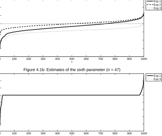
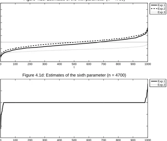
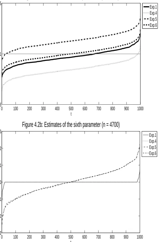
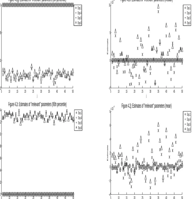
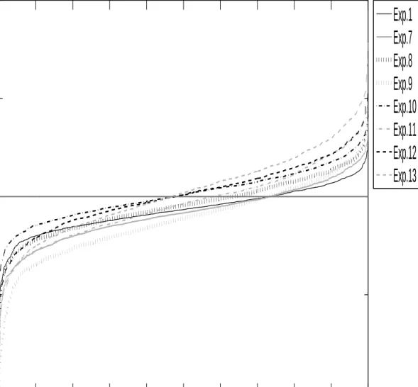
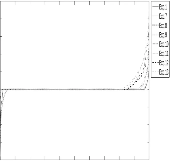
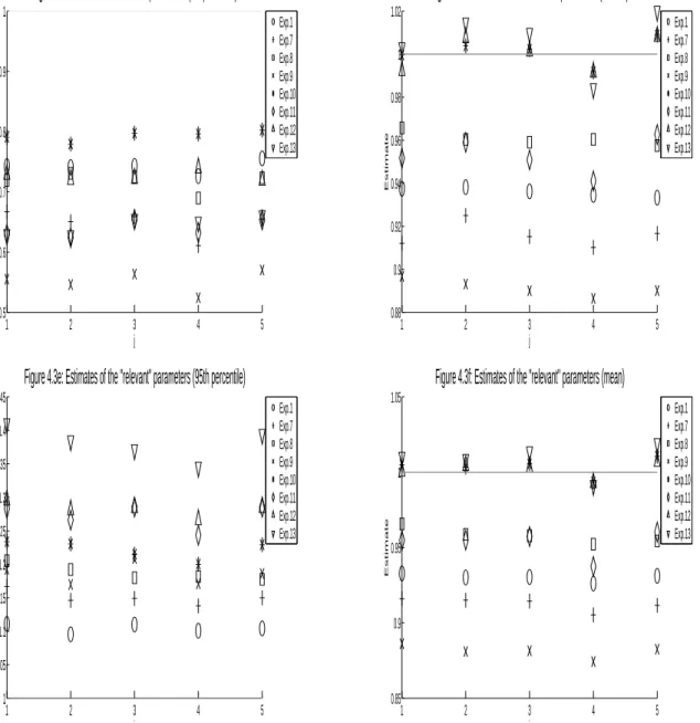
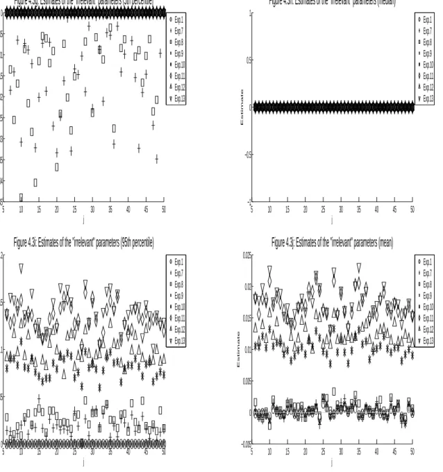
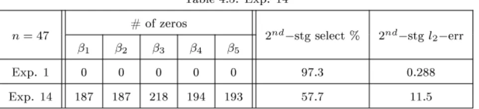
4 Simulations
In this section, simulations are conducted to gain insight on the nite sample performance of the regularized two-stage estimators. I consider the triangular simultaneous equations model (1) and (2) from Section 1 wheredj =d for allj = 1, ..., p,(yi,xTi ,zTi, i,ηi) arei.i.d., and (i,ηi) have the following joint normal
distribution (i,ηi)∼N 0 0 ... 0 , σ2 ρσση · · · ρσση ρσση ση2 0 · · · 0 ... 0 ση2 · · · ... ... ... ... ... 0 ρσση 0 · · · 0 ση2 .
The matrixzTi is ap×dmatrix of normal random variables with identical variancesσz, andzTij is
indepen-dent of (i, ηi1, ..., ηip) for all j = 1, ..., p. With this setup, I simulate 1000 sets of (yi,xTi ,zTi , i,ηi)ni=1
where n is the sample size (i.e., the number of data points) in each set, and perform 14 Monte Carlo
simulation experiments constructed from various combinations of model parameters (d,k1,p, k2, β∗,σ,
and ση), the design of zi, the random matrix formed by the instrumental variables, as well as the types
of rst-stage and second-stage estimators employed (Lasso vs. OLS). For each replication t= 1, ...,1000,
I compute the estimates βˆt of the main-equation parameters β∗, l
2−errors of these estimates, |βˆt−β∗|2,
and selection percentages of βˆt (computed by the number of the elements in βˆt sharing the same sign as
their corresponding elements inβ∗, divided by the total number of elements inβ∗). Table 4.1 displays the
designs of the 14 experiments. For Experiment 1 and Experiments 3-14, I set the number of parameters in
each rst-stage equation d= 100, the number of parameters in the main equation p= 50, the number of
non-zero parameters in each rst-stage equation k1 = 4, the number of non-zero parameters in the main