Sparse Nonlinear MIMO Filtering and Identification

ΣΤΟ ΦΥΣΙΚΟ ΕΠΙΠΕΔΟ 380202

ΑΣΦΑΛΕΙΣ ΑΣΥΡΜΑΤΕΣ ΜΗ-ΓΡΑΜΜΙΚΕΣ ΕΠΙΚΟΙΝΩΝΙΕΣ ΣΤΟ ΦΥΣΙΚΟ ΕΠΙΠΕΔΟ

D2.1 STATE-OF-THE-ART REPORT ON NONLINEAR REPRESENTATION OF SOURCES AND CHANNELS

1

01/02/2012 - 01/05/2013

ΕΘΝΙΚΟ ΚΑΙ ΚΑΠΟΔΙΣΤΡΙΑΚΟ ΠΑΝΕΠΙΣΤΗΜΙΟ ΑΘΗΝΩΝ ΕΘΝΙΚΟ ΚΑΙ ΚΑΠΟΔΙΣΤΡΙΑΚΟ ΠΑΝΕΠΙΣΤΗΜΙΟ ΑΘΗΝΩΝ ΚΑΘΗΓΗΤΗΣ ΝΙΚΟΛΑΟΣ ΚΑΛΟΥΠΤΣΙΔΗΣ

D2.3.1 ΚΕΦΑΛΑΙΟ ΒΙΒΛΙΟΥ: SPARSE NONLINEAR MIMO FILTERING AND IDENTIFICATION

munications

at the Physical Layer

MIS 380202

Deliverable 2.3.1

Sparse Nonlinear MIMO Filtering and

Identification

G. Mileounis and N. Kalouptsidis

date:

March 11, 2014

version:

1.00

and Identification

G. Mileounis and N. Kalouptsidis

Abstract In this chapter system identification algorithms for sparse nonlinear multi input multi output (MIMO) systems are developed. These algorithms are poten-tially useful in a variety of application areas including digital transmission systems incorporating power amplifier(s) along with multiple antennas, cognitive process-ing, adaptive control of nonlinear multivariable systems, and multivariable biolog-ical systems. Sparsity is a key constraint imposed on the model. The presence of sparsity is often dictated by physical considerations as in wireless fading channel– estimation. In other cases it appears as a pragmatic modelling approach that seeks to cope with the curse of dimensionality, particularly acute in nonlinear systems like Volterra type series.

Three identification approaches are discussed: conventional identification based on both input and output samples, semi–blind identification placing emphasis on minimal input resources and blind identification whereby only output samples are available plus a–priori information on input characteristics. Based on this taxonomy a variety of algorithms, existing and new, are studied and evaluated by simulations.

1 Introduction

System nonlinearities are present in many practical situations and remedies based on linear approximations often degrade system performance. A popular model that captures system nonlinearities is Volterra series [69, 71, 77]. This model is employed in communications, digital magnetic recording, physiological systems, control of multivariable systems, etc. Volterra series constitute a class of polynomial models that can be regarded as a Taylor series with memory. An attractive feature of this model is that the unknown parameters enter linearly at the output. On the other

G. Mileounis and N. Kalouptsidis are with the Department of Informatics and Telecommunica-tions, Division of Communications and Signal Processing, University of Athens, Panepistimiopo-lis, 157 84 Ilisia, Greece (e-mail: [email protected]; [email protected])

hand, the number of terms increases exponentially with the order and memory of the model.

Most of the work reported in the literature focuses on modelling and identifi-cation of single input single output (SISO) Volterra systems. When the underlying nonlinear system is a MIMO system, the resulting model is more complicated and has received little attention. MIMO models are addressed in this chapter. Nonlinear MIMO systems involve a large number of parameters to be estimated, which in-creases exponentially with the order, the memory and the number of inputs. There-fore, there is a strong need to reduce complexity by considering those terms that strongly contribute to the outputs. This leads naturally to a sparse approximation of the underlying nonlinear MIMO system. Identification of sparse nonlinear MIMO systems is approached under three different settings: conventional, semi–blind and blind. Blind methods identify the unknown system parameters merely based on the output signals. On the other hand, conventional and semi–blind methods, require a training or a pilot sequence.

The objective of this chapter is twofold. First, it extends existing algorithms for adaptive filtering of SISO models to the MIMO case and demonstrates their appli-cability to nonlinear MIMO systems. Secondly, it presents new algorithms for blind and semi–blind identification of nonlinear MIMO systems excited by finite alpha-bet inputs. The chapter is divided into four sections. The sparse nonlinear MIMO models under consideration are presented in Section 2. Adaptive filters for sparse MIMO systems are discussed in Section 3. Then, algorithms for blind and semi– blind identification are addressed in Section 4. Finally, summary and future work are discussed in Section 5.

2 System Model

MIMO polynomial systems form the basic class of models we shall be working with. These finitely parametrizable recursive structures are defined next. First the basic notation from SISO Volterra series is reviewed. Then MIMO extensions are considered and some special cases of interest are introduced. Finally, various appli-cations which employ MIMO Volterra models are briefly reviewed.

Volterra series constitute a popular model for the description of nonlinear be-haviour [69, 71]. A SISO discrete–time Volterra model has the following form

y(n) = ∞

∑

p=1 ∞

∑

τ1=−∞ ···

∑

∞ τp=−∞ hp(τ1, . . . ,τp) [ p

∏

i=1 x(n−τi) ] . (1)

Each output is formed by weighting the input shifted samplesx(n−τi)and their

products. The weightshp(τ1, . . . ,τp)constitute theVolterra kernelsof orderp. Well

possessedness conditions ensuring that inputs give rise to well defined outputs are given in [51, 13]. If only a finite number of nonlinearities enters Eq. (1), the resulting expression defines a finite Volterra system. Suppose the kernels of a finite Volterra

system are causal and absolutely summable. Then Eq. (1) defines a bounded input bounded output (BIBO) stable system and can be approximated by the polynomial system y(n) = P

∑

p=1 M

∑

τ1=0 ···

∑

M τp=0 hp(τ1, . . . ,τp) [ p

∏

i=1 x(n−τi) ] . (2)

Eq. (2) is parametrized by the finite Volterra kernels and has finite memoryM. A more general result established by Boyd and Chua [14, 13] states that any shift invariant causal BIBO stable system withfading memorycan be approximated by Eq. (2). The fading memory is a continuity property with respect to a weighted norm which penalizes the remote past in the formation of the current output. The reader may consult [13, 14, 51] for more details.

A key feature of Eq. (2) is that it islinear in the parameters. For estimation pur-poses it is useful to write Eq. (2) in matrix form using Kronecker products [15]. Indeed, let x(n) = [x(n),x(n−1),···,x(n−M)]T (the superscriptT denotes the transpose operation) and thepth–order Kronecker power

xp(n) =x_{| {z }}⊗ ··· ⊗x

ptimes

, p=2, . . . ,P.

The Kronecker power contains all pth–order products of the input. Likewiseh= [

h1(·),···,hp(·)

]T

is obtained by treating thep–dimensional kernel as aMp_column

vector. We rewrite Eq. (2) as follows

y(n) =[xT(n)x₂T(n)···xT_p(n)]      h1 h2 .. . hp     =xT(n)h. (3)

Collecting n successive output samples from the above equation into the vector y(n) = [y(1), . . . ,y(n)]results in the following system of linear equations:

y(n) =X(n)h

when

X(n) =[xT(1), . . . ,xT(n)]T.

From a practical viewpoint, Volterra models of order higher than three are rarely considered. This is due to the fact that the number of parameters (∑P_p=1Mp) in-volved in the model of Eq. (2) grows exponentially as a function of the memory size and the order of nonlinearity. To cope with this complexity several sub–families of Eq. (2) have been considered, most notable Wiener, Hammerstein and Wiener– Hammerstein models. In all cases the universal approximation capability is lost. A Wiener system is the cascade of a linear filter followed by a static nonlinearity. If we approximate the static nonlinearity with its Taylor expansion up to a certain order, we obtain the following expression for the output of the Wiener system

y(n) = P

∑

p=1 [ M

∑

τ=0 hp(τ)x(n−τ) ]p . (4)

The Hammerstein system (or memory polynomial) is composed of a memoryless nonlinearity (a Taylor approximation of the static nonlinearity is employed) fol-lowed by a linear filter, and has the following form

y(n) = P

∑

p=1 M

∑

τ=0 hp(τ)xp(n−τ). (5)

A Wiener–Hammerstein or sandwich model is composed of a memoryless nonlin-earity sandwiched between two linear filters with impulse responsesh(·)andg(·)

and is defined as y(n) = P

∑

p=1 M

∑

τ1=0 ···

∑

M τp=0 M_hp+Mgp

∑

k=0 gp(k) p

∏

l=1 hp(τl−k)x(n−τl). (6)

The above models have been employed in a wide range of applications including: satellite, telephone channels, mobile cellular communications, wireless LAN de-vices, radio and TV stations, digital magnetic systems and others [8, 32, 71, 77, 80].

2.1 Nonlinear MIMO systems with universal approximation

capability

The discussion of the previous subsection is next extended to MIMO nonlinear systems. Attention is limited to MIMO polynomial systems. These are finitely parametrizable structures that naturally extend Eq. (2) and preserve a universal ap-proximation capability over a broad class of multivariables systems. We start our discussion by considering cases where either the MIMO system has a single input or a single output. In the end, sparsity is imposed in order to reduce the number of unknown parameters.

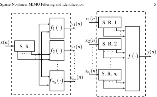
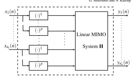
The input–output relationship of nonlinear single input multiple output (SIMO) system is yr(n) = p

∑

p=1 M

∑

τ1=0 ···

∑

M τp=0 h(pr)(τ1, . . . ,τp) p

∏

i=1 x(n−τi) (7)

whereyr(n)is the output associated with therth output signal andh

(r)

p (τ1, . . . ,τp)is

thepth–order Volterra kernelof therth output. The difference between Eq. (2) and Eq. (7) is that a distinct kernelh(pr)(τ1, . . . ,τp)is associated with each output signal

yr(n). This is illustrated in Fig. 1. SIMO systems can be obtained by oversampling

the output signal of a SISO system at a sufficiently high rate and demultiplexing the samples [44].

S. R.

f

1

(

_·

)

x(n)

y

1

(n)

y

2

(n)

y

no

(n)

f

2

(

_·

)

f

n0

(

·

)

S. R. 1

S. R. 2

S. R.

n

i

f

(

·

)

x

1

(n)

y(n)

x

2

(n)

x

ni

(n)

Fig. 1 SIMO and MISO polynomial systems (SR denotes a shift register)

A multiple input single output (MISO) system comprisesniinput signals and a

single output. The input–output of a MISO system has the form

y(n) = P

∑

p=1 ni

∑

t=1 M

∑

τ1=0 ···

∑

M τp=0 hp(τ1, . . . ,τp) p

∏

i=1 xt(n−τi) (8)

wherext(n)is thetth input signal (1≤t≤ni). A shift register (SR) is associated

with each input. The contents of all registers are then converted into the output by means of a feed forward polynomial as shown in Fig. 1.

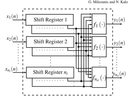
The general MIMO case is readily construed from the above special cases. A MIMO finite support Volterra system withniinputs andnooutputs has the following

form:

yr(n) = fr(x1(n),x1(n−1), . . . ,x1(n−M),···,xni(n),xni(n−1), . . . ,xni(n−M)),

r=1, . . . ,no. (9)

Each outputyr(n)is obtained by a polynomial combination of theni inputs and

their shifts. The parameterM specifies the memory of theni registers associated

with each input. The MIMO finite support Volterra architecture is depicted in Fig. 2. This model is capable of capturing nonlinear effects resulting from any product combinations of theniinputs and their shifts. Expanding fr(·)as a polynomial of

degreePgives rise to the nonlinear MIMO Volterra model with ni inputs and no

outputs defined as yr(n) = P

∑

p=1 ni

∑

t1=1 ···

∑

ni tp=1 M

∑

τ1=0 ···

∑

M τp=0 hp(r,t1···tp)(τ1, . . . ,τp) p

∏

i=1 xti(n−τi) (10)

Shift Register 1

Shift Register 2

Shift Register

n

i

f

1

(

·

)

x

1

(n)

x

2

(n)

x

ni

(n)

y

1

(n)

y

2

(n)

y

no

(n)

f

2

(

·

)

f

no

(

·

)

Fig. 2 A nonlinear MIMO Volterra

whereh(r,t1···tp)

p (τ1, . . . ,τp)is the pth order Volterra kernel associated with therth

output and the(t1···tp)inputs. In this case, the Volterra kernels have

multidimen-sional indices(r,t1···tp).

The above expressions are made complicated by the presence of multiple sum-mations. Kronecker products alleviate this problem. Let

¯

x(n) = [x1(n),x1(n−1), . . . ,x1(n−M),···,xni(n),xni(n−1), . . . ,xni(n−M)]

T

and hence the nonlinear input vector is given by

x(n) = [x¯(n),x¯2(n),···,x¯p(n)]T. (11)

Then Eq. (10) takes the form:

y(n) =Hx(n) (12)

wherey(n) = [y1(n), . . . ,yno(n)]

T _{is the output vector, and the system matrix isH=} [h1:, . . . ,hno:]

T_{, withh}

no:containing all the Volterra kernels associated with therth output. In this case the parameter matrix contains

p

∑

i=1

(ni×M)p

parameters. The MIMO polynomial family of Eq. (9) has a universal approximation capability in the following sense: every nonlinear system with more than one inputs and outputs that is causal, shift invariant, bounded input bounded output stable and has fading memory can be approximated by a MIMO polynomial system of the form given in Eq (10). This assertion is established if the same statement is proved for

MISO systems. The latter follows with straightforward modifications of the proof for the SISO case.

2.1.1 Sparsity aware Volterra kernels

A major obstacle in using Volterra series in practical applications is the exponential growth of the model parameters (as a function of the order, the memory length of the systems and the number of inputs). Thus models of order p>3 and memory lengthM>5, translate into increased computational complexity cost and data re-quirements for identification purposes. For this reason, parsimonious, reduced order alternatives become relevant.

Sparse representations provide a viable alternative. The parameter matrixHin Eq. (12) iss–sparse if the number of non–zero elements is less thans,i.e.

∥vec[H]∥_ℓ0 ={#(i,j):Hi j̸=0} ≤s.

2.2 Special classes of MIMO Nonlinear Systems

In this section, some special classes of MIMO Volterra systems are studied. We start with a simplified version of the MIMO Volterra model. Then structured nonlinear models like Wiener, Hammerstein and Wiener–Hammerstein are extended to the MIMO case. These models are formed by the cascade connection of linear MIMO filters and MIMO static nonlinearities.

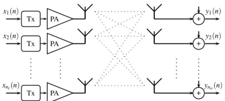
2.2.1 Parallel cascade MIMO Volterra

In MIMO systems the signals from theni inputs interact with each other and the

resulting mixture is received at each output. A special case of Eq. (10) results when the MIMO system obtains from the parallel connection of SISO systems, where each SISO system is often referred to as a path or parallel system. If the path between each input and each output is modelled as a Volterra system, then therth output is expressed as follows yr(n) = P

∑

p=1 ni

∑

t=1 M

∑

τ1=0 ···

∑

M τp=0 h(pr,t)(τ1, . . . ,τp) p

∏

i=1 xt(n−τi) (13)

whereh(pr,t)(τ1, . . . ,τp)is thepth–order Volterra kernelbetween thetth input and

therth output for allt=1, . . . ,niandr=1, . . . ,no. The above model does not

al-low product combinations along different inputs. Instead each input is nonlinearly transformed and then all different inputs are linearly mixed. Such a model can be considered as a parallel cascade ofniSIMO Volterra models.

Tx Tx Tx PA PA PA + + + xn_i(n) x₂(n) x₁(n) yn_o(n) y₂(n) y₁(n)

Fig. 3 An example of a parallel cascade MIMO Volterra channel

Eq. (13) can be written in a form identical to that of Eq. (12). Define thetth input regressor vector as

x(t)(n) = [x(t)(n),x(t)(n−1), . . . ,x(t)(n−M)]T. Then the linearly mixed input vector takes the form:

x(n) = [x(₁1)(n),x₂(1)(n), . . . ,x(p1)(n),···,x(₁ni)(n),x₂(ni)(n), . . . ,x(pni)(n)]T.

The total number of parameters of the above linearly mixed model is

ni p

∑

i=1

Mp

and is considerably reduced when compared to the general case.

The linearly mixed model finds application in nonlinear communications. Com-munication nonlinearities can be categorized into the following three types: trans-mitter nonlinearity (due to nonlinearity in amplifiers), inherent physical channel nonlinearity, and receiver nonlinearity (e.g., due to nonlinear filtering). The power amplifier (PA) (which is located at the transmitter) constitutes the main source of nonlinearity. In a system equipped with multiple transmit antennas, each transmit-ter amplifies the signal. Amplifiers often operate near saturation to achieve power efficiency. In those cases they introduce nolinearities which cause interference and reduce spectral efficiency. At the receiver end, each antenna receives a linear su-perposition of all transmitted signals, as illustrated in Fig. 3. It should be pointed out that the nonlinear effects are applied to each input signal individually prior to mixing the transmitted signals.

Linear

MIMO System

H

(

·

)

1

(

·

)

p

x

1

(

n

)

x

_ni

(

n

)

y

1

(

n

)

y

no

(

n

)

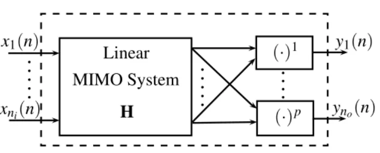
Fig. 4 A MIMO Wiener System

2.2.2 Block–structured classes of nonlinear MIMO systems

TheMIMO Wiener modelis shown in Fig. 4. It consists of a linear MIMO system in cascade with a polynomial nonlinearity for each output. The output is given by

yr(n) = P

∑

p=1 ni

∑

t1=1 ···

∑

ni tp=1 M

∑

τ1=0 ···

∑

M τp=0 p

∏

i=1 h(r,ti) p (τi)xti(n−τi). (14) This model is a special subclass of the MIMO Volterra series model. The relation-ship between thepth–order Volterra kernel andpth–order Wiener kernel is

h(rt1···tp) p (τ1, . . . ,τp) = p

∏

i=1 h(r,ti) p (τi).

Thus a MIMO Wiener model is equivalent to a MIMO Volterra system with separa-ble kernels. The MIMO Hammerstein model is one of the simplest and most popular subclasses of MIMO Volterra models. As the diagram of Fig. 5 shows, the MIMO Hammerstein is a cascade connection of a static polynomial nonlinearity for each input connected in series by a linear MIMO system. It consists of the same building blocks as the Wiener model, but connected in reverse order. It has the following form: yr(n) = P

∑

p=1 ni

∑

t=1 M

∑

τ=0 h(pr,t)(τ)xp(n−τi). (15)

Thepth–order Volterra kernel of a Hammerstein model is given by

h(rt1···tp)

p (τ1, . . . ,τp) =hp(τ1)δ(τ2−τ1)···δ(τp−τ1)δ(t2−t1)···δ(tp−t1) (16)

A Hammerstein system prohibits product interactions between different inputs and hence corresponds to a diagonal MIMO Volterra model.

We finally consider the case where the MIMO Volterra kernels have factorable form: h(rt1···tp) p (τ1, . . . ,τp) = Mh+Mg

∑

k=0 gr_p(k) p

∏

i=1 hti p(τi−k)

(

·

)

1

(

·

)

p

Linear MIMO

System

H

y

₁

(

n

)

y

no

(

n

)

x

₁

(

n

)

x

_ni

(

n

)

(

·

)

1

(

·

)

p

Fig. 5 A MIMO Hammerstein system

Substituting the above form into Eq. (10), we obtain:

yr(n) = P

∑

p=1 ni

∑

t1=1 ···

∑

ni tp=1 M

∑

τ1=0 ···

∑

M τp=0 Mh+Mg

∑

k=0 gr_p(k) p

∏

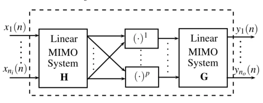
i=1 hti p(τi−k)xti(n−τi). (17) Thepth–order kernel corresponds to a cascade connection of a linear MIMO system followed by a memoryless nonlinearity followed by another linear MIMO system and is known asMIMO Wiener–Hammersteinor sandwich model. In its simplest form a MIMO Wiener–Hammerstein system has a sandwiched structure with a sin-gle input sinsin-gle output static nonlinearity placed between a MISO and a SIMO linear systems. In the general case, illustrated in Fig. 6, the two linear filters can have ar-bitrary input and output dimensions. Compatibility is secured by proper dimension-ing of the MIMO static nonlinearity. The Wiener–Hammerstein has been widely employed in satellite transmission, where both the earth station and the satellite re-peater employ (nonlinear) power amplifiers. In such cases the signal bandwidth is very carefully defined depending on the application so that the output signal contains only spectral components near the carrier frequencyωc. This leads to theMIMO

baseband Wiener–Hammersteinsystem [8, Ch. 14], given by

yr(n) = ⌊P−1 2 ⌋

∑

p=1 ni

∑

t1=1 ···

∑

ni t2p+1=1 M

∑

τ1=0 ···

∑

M τ2p+1=0 Mh+Mg

∑

k=0 gr_p(k) p

∏

i=1 (18) ×p

∏

+1 i=1 hti 2p+1(τi−k)xti(n−τi) 2p+1

∏

j=p+2 ht_2pj ₊₁(τj−k)xt∗j(n−τj) where⌊·⌋denote the floor operation. The above representation only considers odd– order powers with one more unconjugated input than conjugated input. This way the output does not create spectral components outside the frequency band of interest.

Linear

MIMO

H

(

·

)

1

(

·

)

p

x

1

(

n

)

x

ni

(

n

)

y

1

(

n

)

y

no

(

n

)

System

Linear

MIMO

G

System

Fig. 6 A MIMO Wiener–Hammerstein system

2.3 Practical applications of MIMO Volterra systems

Nonlinear MIMO systems are found in a range of communication and control ap-plications. These are shortly reviewed next.

2.3.1 Nonlinear communication systems

Communication systems equipped with multiple transmit and/or receive antennas are MIMO systems that help provide spatial diversity. Exploitation of spatial diver-sity results in higher capacity and performance improvements in interference reduc-tion, fading mitigation and spectral efficiency. Most of existing MIMO schemes are limited to linear systems. However, in many cases, system nonlinearities are present and possible remedies based on linear MIMO approximations degrade performance significantly.

In a communication system, there are often limited resources (power, frequency, and time slots) which have to be efficiently shared by many users. Quite often in practice we encounter a situation whereby the number of users exceeds the num-ber of available frequency or time slots. In infrastructure–based networks, a base station or an access point is responsible for allocating resources among the users, thereby reducing the access delays/transmission latency and improving quality–of– service (QoS). This is established through a variety of multiple accessschemes. Two key multiple access technologies suitable for higher data rates are: orthogonal frequency–division multiple access (OFDMA) and code–division multiple access (CDMA).

OFDMA dynamically allocates resources both in frequency (by dividing the available bandwidth into a number of subbands, called subcarriers) and in time (via OFDM symbols). The transmission system assigns different users to groups of orthogonal subcarriers and thus allows them to be spaced very close together with no overhead as in frequency division multiple access. Furthermore it prevents interference between adjacent subcarriers. OFDMA has been implemented in sev-eral wireless communication standards (IEEE 802.11a/g/n wireless local area net-works (WLANs), IEEE 802.16e/m worldwide interoperability for microwave access

(WiMAX), Hiperlan II), high–bit–rate digital subscriber lines (HDSL), asymmetric digital subscriber lines (ADSL), very high-speed digital subscriber lines (VHDSL), digital audio broadcasting (DAB), digital television and high-definition television (HDTV).

OFDMA is capable of mitigating intersymbol interference (ISI), (due to mul-tipath propagation) using low–complexity/simple equalization structures. This is achieved by transforming the available bandwidth into multiple orthogonal narrow-band subcarriers, where each subcarrier is sufficiently narrow to experience rela-tively flat fading. Nevertheless, OFDM is sensitive to synchronization issues and is characterized by high peak–to–average–power–ratio (PAPR), caused by the sum of several symbols with large power fluctuations. Such variations are problematic because practical communication systems are peak powered limited. In addition, OFDM transceivers are intrinsically sensitive to power amplifier (PA) nonlinear dis-tortion [38], which dissipates the highest amount of power. One way to avoid nonlin-ear distortion is to operate the PA at the so–called “back–off” regime which results in low power efficiency. The trade–off between power efficiency and linearity mo-tivated the development of signal processing tools that cope with MIMO–OFDM nonlinear distortion [40, 45, 38].

CDMA is based upon spread spectrum techniques. It plays an important role in third generation mobile systems (3G) and has found application in IEEE 802.11b/g (WLAN), Bluetooth, and cordless telephony. In CDMA multiple users share the same bandwidth at the same time through the use of (nearly) orthogonal spread-ing codes. The whole process effectively spreads the bandwidth over a wide fre-quency range (using pseudo–random code spreading or frefre-quency hopping) several magnitudes higher than the original data rate. Two critical factors that limit the per-formance of CDMA systems are interchip and intersymbol interference (ICI/ISI), due to multipath propagation, mainly because they tend to destroy orthogonality between user codes and thus prevent interference elimination. Suppression of the detrimental effects of interference (ICI and ISI) get further complicated when non-linear distortion is introduced due to power amplifiers. The combined effects of ICI, ISI and nonlinearities are comprehensively examined in [40, 67]. However, as recently illustrated in [22], the CDMA system model is sparse due to user inac-tivity/uncertainty, timing offsets and multipath propagation. CDMA system perfor-mance can be expected to improve further if nonlinearities along with sparse ICI/ISI are revisited.

2.3.2 MIMO nonlinear physiological systems

In several physiological applications it is mandatory to gain as much insight infor-mation is possible about the functioning of the system. It is well documented in the biomedical literature that nonlinear systems can significantly enhance the quality of modelling [57, 80]. Very often linear approximations discard significant infor-mation about the nonlinearities. For this reason, several physiological systems like sensory systems (cockroach tactile spine, auditory system, retina), reflex loops (in

the control of limb and eye position), organ systems (heart rate variability, renal auto–regulation) and tissue mechanics (lung tissue, skeletal muscle) have been ap-proached via nonlinear system analysis using Volterra series [57, 80]. Many of the above physiological systems receive excitation from more than one input, and hence leads naturally to MIMO Volterra models.

2.3.3 Control applications

Quite often control applications exhibit multivariable interactions and nonlinear be-haviour, which make the modelling task and design more challenging. Examples of such control systems include: multivariable polymerization reactor [32], fluid catalytic cracking units (FCCU) [83, 84], and rapid thermal chemical vapor decom-position systems (RTCVD) [72].

Multivariable polymerization reactor aims to control the reactor temperature at the unstable steady state by manipulating the cooling water and monomer flow rates. MIMO Volterra models have been employed to capture/track the nonlinear plant output [32]. The FCCU unit constitutes the workhorse of modern refinery and its purpose is to convert gas oil into a range of hydrocarbon products. The major challenges related to FCCU are its internal feedback loops (interactions) and its highly nonlinear behaviour [84]. RTCVD is a process used to deposit thin films on a semiconductor wafer via thermally activated chemical mechanisms. Process and equipment models for RTCVD consist mainly of balance equations for conserva-tion of energy, momentum and mass, along with equaconserva-tions that describe the relevant chemical mechanisms. An important characteristic of RTCVD systems is their wide region of operation, which requires excitation of the system with as many modes as possible and hence a nonlinear MIMO system becomes relevant. A major challenge in all the above control applications is the large number of parameters required by the nonlinear MIMO models.

3 Algorithms for sparse multivariable filtering

Adaptive filters with a large number of coefficients are often encountered in multi-media signal processing, MIMO communications, biomedical applications, robotics, acoustic echo cancellation, and industrial control systems. Often, these applications are subject to nonlinear effects which can be captured using the models of Section 2. The steady–state and tracking performance of conventional adaptive algorithms can be improved by exploiting the sparsity of the unknown system. This is achieved via two different strategies [82]. The first is based onproportionate adaptive filters, which update each parameter of the filter independently of the others by adjusting the step size in proportion to the magnitude of the estimated filter parameter. In this manner, the adaptation gain is “proportionately” redistributed among all parameters, emphasizing the large coefficients in order to speed up convergence and increase the

overall convergence rate. The second strategy is motivated by thecompressed sens-ingframework [16, 76, 36]. Compressed sensing approaches follow two main paths: (a) theℓ1minimization (also referred to as basis pursuit) and (b) greedy algorithms

(matching pursuit). Basis pursuit penalizes the cost function by theℓ1–norm of the

unknown parameter vector (or a weighted ℓ1–norm), as the ℓ1–norm (unlike the

ℓ2–norm) favours sparse solutions. These methods combine conventional adaptive

filtering algorithms such as LMS, RLS, etc with a sparsity promoting operation. Ad-ditional operations include the soft–thresholding (originally proposed for denoising by D. L. Donoho in [30]) and the metric projection onto theℓ1–ball [25, 33]. Greedy

algorithms, on the other hand, iteratively compute the support set of the signal and construct an approximation of the parameters until convergence is reached. Propor-tionate adaptive filtering was developed by D. L. Duttweiler in 2000 [34]. There-after, a variety of improved versions has been proposed [64]. A connection between proportionate adaptive filtering and compressed sensing is discussed in [64].

3.1 Sparse multivariable Wiener filter

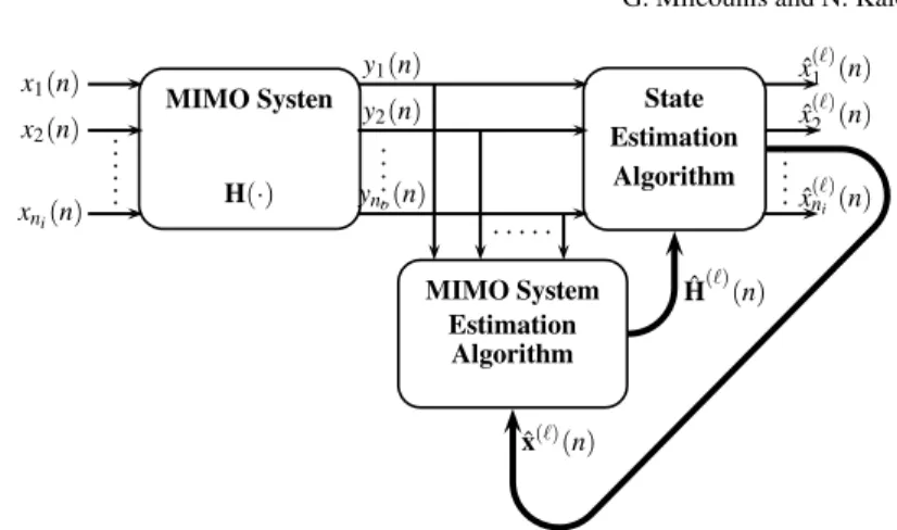
The block diagram of Fig. 7 shows a discrete–time MIMO filter withniinputs and

nooutputs [7, 47]. The outputy(n), the impulse response matrix Hand the input

x(n)are related by:

y(n) =Hx(n) +v(n) (19)

wherex(n)is defined in Eq. (11) andv(n) = [v1(n),v2(n),···,vno]

T _{is a Gaussian}

white noise vector. The following equation shows therth output signal

yr(n) = ni

∑

τ=1 hT_rτx_τ(n) +vr(n) (20) =hT_r:x(n) +vr(n), r=1, . . . ,no. (21) and H=    hT₁₁ ··· hT_1n i .. . . .. ... hT_n o1··· h T noni   =    hT_1: .. . hT_no:   . (22)

An adaptive process is employed to cause therth output to agree as closely as possible with the desired response signaldr(n). This is accomplished by comparing

the outputs with the corresponding desired responses and by adjusting the parame-ters to minimize the resulting estimation error. More specifically, given an estimate

ˆ

H(n)ofHthe estimation error is:

er(n) =yr(n)−dr(n) =yr(n)−hb T

r:(n)x(n), r=1, . . . ,no (23)

1 x1(n) x2(n) xn_i(n) Discrete–Time Filter H y1(n) y2(n) yno(n) + + + d1(n) d2(n) dno(n) e1(n)e2(n) en_o(n) Fig. 7 MIMO filtering

e(n) =y(n)−Hb(n)x(n). (24) The performance of a filter is assessed by a functional of the estimation error. LS filters, minimize the total squared error:

JLS(n) = n

∑

i=1 eH1(i)e(i) = n

∑

i=1 ∥e(i)∥2_ℓ 2 (25) = no

∑

r=1 Jhr:(n). (26)

The optimum MIMO filter is given by the system of linear equations

Ho(n)Rxx(n) =Pyx(n) (27)

whereRxx(n)is the input sample covariance matrix (which has block Toeplitz struc-ture) with Rxixj(n) = n

∑

t=1 xi(t)xHj(t), and Pyx(n) = n

∑

i=1 y(i)xH(i) =[pyx1(n)pyx2(n)··· pyxni(n) ] . (28)

Under broad conditions the solutions of Eq. (27) tends to be the optimum mean squared filter (occasionally referred to as Wiener filter) that minimizes the mean squared errorE{∥e(i)∥2

ℓ2}and satisfies the system of linear equations given by Eq. (27) (Pyx(n) =E{y(i)xH(i)} andRxx(n) =E{x(i)xH(i)}). Equation (27) can be decomposed innoindependent MISO equations each corresponding to an output

signal [9, 47], as follows:

hr:,o(n)Rxx(n) =pyrx(n), r=1, . . . ,no. (29)

Consequently, minimizing JLS(n)or minimizing eachJhr:(n)independently gives exactly the same results.

Two popular algorithms for adaptive filtering are the Least Mean Squares (LMS) algorithm and the Recursive Least Squares (RLS) algorithm. The LMS follows a stochastic gradient method and has a computationally simpler implementation. On the other hand, the more complex RLS has better convergence rate.

The LMS seeks to minimize the instantaneous error

JLMS(n) =eH(n)e(n). (30)

The LMS estimate for the impulse response matrix His based on the following update equation:

H(n) =H(n−1) +µe(n)xH(n) (31) where the step sizeµdetermines the convergence rate of the algorithm. To achieve convergence in the mean to the optimal Wiener solution,µshould be chosen so that:

0<µ< 2

M∑ni

τ σx2_τ

. (32)

The RLS algorithm attempts to minimize the exponentially weighted cost func-tion: JRLS(n) = n

∑

t=1 λn−t_eH_{(t)e(t) (33)}

whereλ denotes the forgetting factor. The RLS estimates are updated as follows: H(n) =H(n−1) +e(n)kT(n) (34) where k(n) = R −1 xx(n)x∗(n) λ+xT_(n)R−1 xx(n)x∗(n)

is known as theKalman gain[46, 70]. The matrix inversion lemma [46, 70], leads to:

R−_xx1(n) =λ−1R−_xx1(n−1)−k(n)xT(n)R_xx−1(n−1). (35)

3.2

L

1

constrained adaptive filters

These algorithms are based on the minimization of cost functions penalized by the ℓ1–norm (or a weightedℓ1–norm or an approximateℓ0–norm) and are inspired by

the fact that theℓ1–norm promotes sparse solutions and is the best convex relaxation

Table 1 ZA–LMS Algorithm Algorithm description H(0)=0 Forn:=1,2,. . .do 1: e(n) =d(n)−H(n−1)x(n) 2: H(n) =H(n−1) +µe(n)xH(n)−γsgn(H(n−1)) End For 3.2.1 LMS–type filters

The sparse cost function combines the instantaneous error with a sparseness induc-ing penalty term

JZA−LMS(n) =

1 2

(

eH(n)e(n))+τpen(H(n)) (36)

τ is a positive scalar regularization parameter which provides a trade–off between penalization and signal reconstruction error. The most well–known sparsity induc-ing penalty term is theℓ1–norm (pen(H(n)) =∥vec[H(n)]∥ℓ1). Although a large portion of the literature focuses on theℓ1–norm there are other functions which

pro-mote sparsity [48, 42]. In fact, any penalization term, with pen(H(n))being sym-metric, monotonically non–decreasing, and with decreasing derivative will serve the same purpose [36].

Sparse LMS–type variants obey the following updating scheme

   new parameter estimate   =    old parameter estimate   + { stepsize} { new in f ormation } +    zero attraction term   

where the new information term is the error vector between the outputs of the fil-ter and the desired signal vector. TheZero–Attraction(ZA) term is a norm related regularization function which exerts an attraction to zero on small parameters. Con-vergence of the recursion may be slow because the two parts are hard to balance. This issue is addressed in some detail later in the subsection.

The first of this type of algorithms (originally developed in [18, 19] for SISO systems) minimizes Eq. (36). The filter parameter matrix is updated by

H(n) =H(n−1)−µ∇JZA−LMS(n)

=H(n−1) +µe(n)xH(n)−γ∇spen(H(n−1)) (37) where∇spen(H(n−1))is the sub–gradient of the convex function pen(H(n−1)),

γ =µτ is the regularization parameter. In the adaptive filtering contextγ is also referred to as regularization step size. Usually the regularization step size is fine tuned offline (via exhaustive simulations) or in an ad–hoc manner. A systematic approach to choosingγis developed in [19].

Under the standard compressive sensing setting, the penalty is given by the ℓ1–norm and the resulting algorithm is shown in Table 1. Note that sgn(·) is a

component–wise sign functiondefined as

sgn(Hi j) = {

Hi j/|Hi j| ifHi j̸=0,

0 ifHi j=0.

(38)

It is well known that the LMS, in a stationary environment, achieves unbiased con-vergence in the mean to the Wiener solution (using the independence assumption) [46]. However, unlike the conventional LMS, ZA–LMS leads to a biased behaviour [48], that is

E[H(n)] =Ho−γ

µE[H(n)]Rxx−1(n), asn→∞ (39) Recall that a key difference between theℓ0 norm and theℓ1norm penalty, is that

theℓ1norm depends on the magnitudes of the non–zero components, whereas the

ℓ0–norm penalty does not. As a result, the larger a component is, the heavier it is

penalized by theℓ1penalty. To overcome this often unfair penalization two different

penalty terms are introduced in the conventional LMS cost function. Both form better approximations to theℓ0norm. The first is based on an approximation of the

step function [79] pen(H(n)) =

∑

i ( 1−exp−a′|veci[H(n)]| ) (40)

wherea>0 is a parameter that must be chosen. The authors in [49] reduce the com-putational complexity of the resulting zero attraction term by considering the first order Taylor series expansion of exponential functions. The resulting filter update iteration (namedℓ0–LMS) becomes

H(n) =H(n−1) +µe(n)xH(n)−γa(1−a|H(n−1)|)₊sgn(H(n−1)) (41) where(x)+=max{x,0}. Motivated by the re–weighted ℓ1 cost function in [17],

the authors in [18] follow this approach in order to reinforce the ZA–LMS by re– weighting the sparse penalty term. The proposed penalty term is given by

pen(H(n)) =

∑

i log ( 1+ε′−1|veci[H(n)]| ) . (42)

According to the stochastic gradient approach, the resulting filter update iteration is H(n) =H(n−1) +µe(n)xH(n)−γ sgn(H(n−1))

1+ε|H(n−1)| (43)

and the algorithm is named RZA–LMS. Small coordinates of the estimated ma-trix are more heavily weighted (by 1/(1+ε|H(n−1)|)) towards zero, and small weights encourage larger coordinates. As a result, the bias of the mean value of the converged matrix for RZA–LMS is reduced.

So far we have examined how to solve the penalized LMS cost function of Eq. (36) by embedding additional terms to the update formula. A different viewpoint arises by consideringproximity splittingmethods [21]. The proximity operator of a (possibly non–differentiable) convex functionΩ(H(n))is defined as

prox_τ,Ω(H(n)):=argmin H(n) 1 2τ∥Y(n)−H(n)∥ 2 ℓ2+Ω(H(n)).

Proximity operators are the main ingredient of proximal methods [21] which arise in many well–known algorithms (e.g., iterative thresholding, projected Landweber, projected gradient, alternating projections, alternating-direction method of multipli-ers, alternating split Bregman). In these algorithms, proximal methods can be un-derstood as generalizations of quasi–Newton methods to non–differentiable convex problems. An important example is the Iterative Thresholding procedure [24] which solves problems of the form:

min

H J(H) +Ω(H), (44)

J(H)is differentiable with Lipschitz gradient. By iterating the fixed point equation

H(n):= prox_µ,Ω | {z } backward step [H(n−1)−µ∇J(H(n−1))] | {z } forward step (45)

for values of the step–size parameterµin a suitable bounded interval. This scheme is known as a forward–backward splitting algorithm. In some cases, the proximity operator prox_µ,Ω can be evaluated in closed form.

If we consider the minimization of the cost functionJZA−LMS (defined in Eq.

(36)) with pen(H(n)) =∥vec[H(n)]∥ℓ1 we obtain min H 1 2|e(n)| 2_{+τ∥vec[H(n)]∥} ℓ1.

We observe that the above problem is a special case of Eq. (44) with

{

J: H7→1₂|e(n)|,

Ω: H7→τ∥vec[H(n)]∥_ℓ1.

Then it follows from [21, 61] that the proximity operator prox_µ,Ω leads to a non-linear component–wise shrinkage operation known as soft–thresholding [30]. The component-wisesoft–thresholdingoperation is defined by

Sτ[Hi j] =      Hi j−τ ifHi j≥τ, 0 if|Hi j| ≤0, Hi j+τ ifHi j≤τ (46)

or in compact notationS_τ[Hi j] =sgn(Hi j) (|Hi j| −τ)₊[30]. This operation shrinks

coefficients above the threshold in magnitude by an amount equal toτ. An instanta-neous proximity operation leads to the soft–thresholded LMS filter

H(n) =S_τ[H(n−1) +µe(n)xH(n)]. (47) Detailed analysis of the dynamics of Eq. (47) in its batch format, has shown that the algorithm converges initially relatively fast, then it overshoots theℓ1penalty, and it

takes very long to re–correct back. To avoid such a behaviour in the adaptive case, we force the successive iterates to remain within a particular ℓ1 ballBR [25]. To

achieve this the thresholding operation is replaced by a projectionPBR , where, for any closed convex setC and anyH, the projectionP_C(H)is defined as the unique point inC for which theℓ2distance toHis minimal. We thus obtain the projected

LMS onℓ1ball

H(n) =PBR

[

H(n−1) +µe(n)xH(n)]. (48) The projection operatorPBR[Hi j(n)]is obtained by a suitable thresholding ofHi j(n), given PBR[Hi j] =     

PBR[Hi j] =Sµ[Hi j] if∥vec[H(n)]∥ℓ1 >R, and chooseµ such that∥S_µ[vec[H(n)]]∥ℓ1=R

PBR[Hi j] =S0[Hi j] if∥vec[H(n)]∥ℓ1 ≤R.

(49)

Using proximal splitting methods other types of adaptive filters, such as NLMS/APA and Adaptive Projection algorithms, can be modified to promote sparsity [54, 61].

3.2.2 RLS–type filters

Sparse RLS–type filters modify the RLS cost function (33) by the addition of a sparsifying term:

JZA−RLS(n) =

1

2JRLS(n) +τpen(H(n)). (50) The regularization parameterτ controls sparsity and weighted squared error. The sparse RLS filter can be seen as an adaptive version of Gauss–Newton or Newton– Raphson search with sparse updates [55]. Alternatively, the RLS algorithm is a spe-cial case of a Kalman filter [46, 70]. The main recursion takes the following form:

   new parameter estimate   =    old parameter estimate   + { Kalman gain } { innovation vector } +    zero attraction term   

The correction term is proportional to the innovation error vector between the pre-dicted observations and the actual observations. The coefficients of this correction are provided by the Kalman gain. For the regularized Recursive Least Square

prob-lem of Eq. (50) the solution of the Wiener equation takes the form [35]:

H(n) =Pyx(n)C(n)−γ(1−λ)∇spen(H(n−1))C(n) (51) whereC(n) =R−1

xx(n),λ ∈(0,1)is the forgetting factor and∇spen(H(n−1))is a subgradient sinceJZA−RLS(n)is non–differentiable at any point whereHi j(n) =

0 [10, p. 227]. The exponentially weighted autocorrelation and cross–correlation matrices are recursively updated as:

Rxx(n) = n

∑

t=1 λn−t_x(t)xH_{(t) =λR} xx(n−1) +x(n)xH(n) (52) Pyx(n) = n

∑

t=1 λn−t_y(t)xH_{(t) =λP} yx(n−1) +y(n)xH(n). (53) The regularized RLS filter relies on the following recursion [35]:

H(n) =H(n−1) +e(n)kT(n)−γ(1−λ)∇spen(H(n−1))C(n) (54) where the regularization parameterγ is usually fine tuned offline or using the se-lection rule proposed in [35] (for white inputs). In this case the corresponding sub-gradient is∇s∥Hi j(n−1)∥ℓ1 =sgn(Hi j(n−1)). Instead we may utilize the penalty functions, suggested in the LMS context, given by Eqs. (40) and (42).

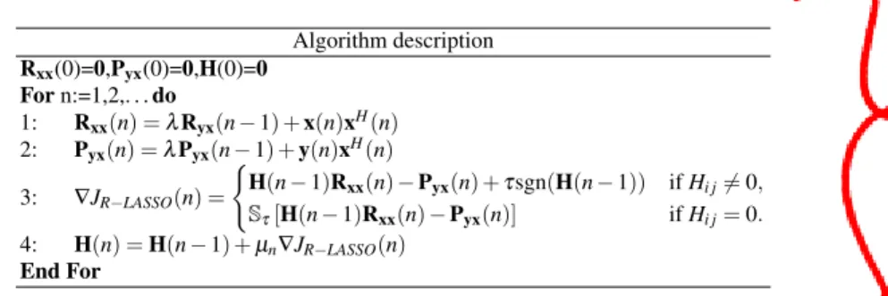
RLS algorithms are developed based on the batch LASSO estimator in [4, 3]. This method modifies the LASSO cost function to include a forgetting factor:

argmin H(n) 1 σ2 n

∑

i=1 λn−i_{∥y(i)−H(i)x(i)∥}2 ℓ2+γpen(H(n)). (55) The first order subgradient based optimality conditions for the exponentially weighted LASSO cost imply:

{

∇i jJRLS(n) +τsgn(Hi j(n)), ifHi j(n)̸=0

|∇i jJRLS(n)| ≤τ ifHi j(n) =0.

These conditions and the value of∇i jJRLS(n)are used to define a pseudo–gradient

for each component ofH[2]. The pseudo–gradient ofJR−LASSO(n)is the element of

the sub–differential ofJR−LASSO(n)atH(n)with minimum norm and is given by:

∇i jJR−LASSO(n) =          ∇i jJRLS(n) +τsgn(Hi j(n)), ifHi j(n)̸=0 ∇i jJRLS(n) +τ ifHi j(n) =0,∇i jJRLS(n)<−τ ∇i jJRLS(n)−τ ifHi j(n) =0,∇i jJRLS(n)>τ 0 ifHi j(n) =0,−τ≤∇i jJRLS(n)≤τ.

In the first case the function is differentiable, so the pseudo–gradient is simply the gradient with respect toi j(the only element of the sub–gradient). In the

remain-Table 2 R-LASSO Algorithm Algorithm description Rxx(0)=0,Pyx(0)=0,H(0)=0 Forn:=1,2,. . .do 1: Rxx(n) =λRyx(n−1) +x(n)xH(n) 2: Pyx(n) =λPyx(n−1) +y(n)xH(n) 3: ∇JR−LASSO(n) = { H(n−1)Rxx(n)−Pyx(n) +τsgn(H(n−1)) ifHi j̸=0, Sτ[H(n−1)Rxx(n)−Pyx(n)] ifHi j=0. 4: H(n) =H(n−1) +µn∇JR−LASSO(n) End For

ing three cases we obtain the minimum–norm solution by the soft–thresholding op-eration to ∇i jJRLS(n). The global solution to the smooth part of the LASSO cost

function is the Wiener equation, where the autocorrelation and the cross–correlation matrices are recursively updated from Eqs. (52) and (53).

Using the subgradient, an instantaneous subgradient descent strategy is employed for online updating as follows

H(n) =H(n−1) +µ∇JR−LASSO(n). (56)

The Recursive LASSO (R–LASSO) filter outlined here is summarized in Table 2. As with the batch LASSO estimator, the R–LASSO does not necessarily converge to the true parameterHsince it fails to recover the correct support and at the same time estimate the non–zero entries ofHconsistently [4].

In order to improve the performance of the R–LASSO filter, one could use a dif-ferent penalty term which is signal dependent and weights difdif-ferently the entries in theℓ1norm, that is pen(H(n)) =∑iwτ(|veci

[ b

HRLS(n) ]

|)∥veci[H(n)]∥ℓ1. By gen-eralizing theSmoothly Clipped Absolute Deviation(SCAD) regularizer introduced for the batch weighted LASSO estimator to its adaptive case, the following weight function is obtained

w_τ(|veci[H(n)]|) =

[ατ− |veci[H(n)]|]+

τ(α−1) u(|veci[H(n)]|−τ)+u(τ−|veci[H(n)]|)

u(·)stands for the step function andα is usually set to 3.7. The reweighted LASSO estimator (RW–LASSO) places higher weight to small entries, and lower weight to entries with large amplitudes. In fact, the estimates of size less thanτ are penal-ized as in R–LASSO, while estimates betweenτandατ are penalized in a linearly decreasing manner. Estimates larger thanατ are not penalized at all. The imple-mentation of RW–LASSO is established using an instantaneous pseudo–gradient descent strategy, similar to R–LASSO. The downside of this estimator is its high complexity because it requires running in parallel an RLS algorithm to supply the needed weights.

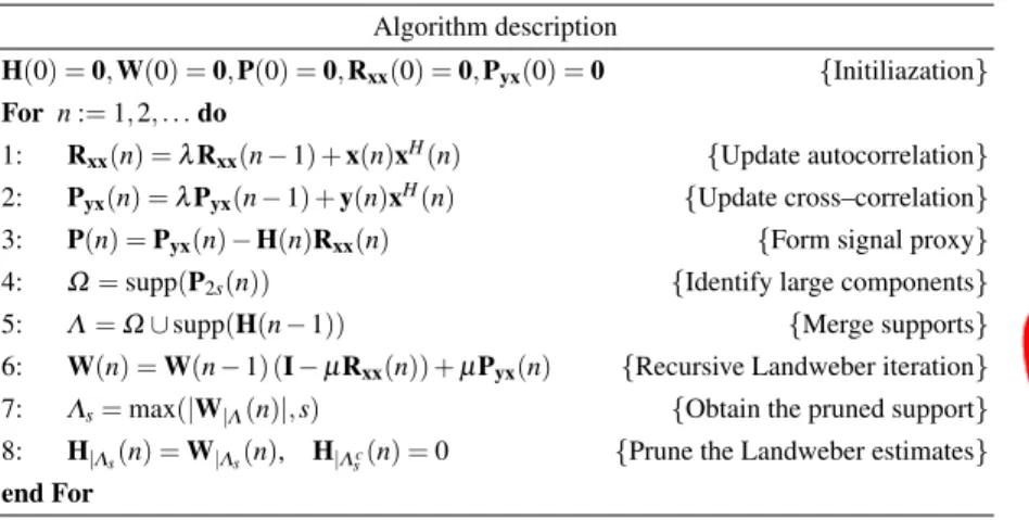
Table 3 spaRLS Algorithm Algorithm description Rxx(0)=0,Pyx(0)=0,H(0)=0 Forn:=1,2,. . .do 1: Rxx(n) =λRxx(n−1) +a 2 σ2x(n)x H_(n) 2: Pyx(n) =λPyx(n−1) +a 2 σ2y(n)x H_(n) 3: Repeat 4: Gb(λ)(n) =Hb(λ)(n) (I−Rxx(n)) +Pyx(n) 5: Hb(λ)(n) =S_γa2 [ b G(λ)(n) ] 6: Untilλ=k End For

A different viewpoint to sparse RLS algorithms is provided in [5] (and its MIMO extension in [53]). This approach makes use of the Expectation Maximization (EM) method [27] to derive an adaptive filter that solve a penalized Maximum Likeli-hood problem. The penalized Recursive Least Squares problem may be posed as a penalized Maximum Likelihood problem [41]. This penalized ML problem can be efficiently solved by an EM algorithm following the noise decomposition idea (proposed in [41]) in order to divide the optimization problem into a denoising and a filtering problem. Consider the following decomposition forV(n)

V(n) =αV1(n)X(n) +V2(n). (57)

The noise matrices are ensembles of Gaussian–distributed random matrices V1(n) = (0,Ini⊗Ino)

V2(n) = (

0,(σ2Λ−1−α2X(n)XH(n))T⊗Ino

)

whereΛ:=diag[λn−1···λ0]andαis a constant which must fulfilα≤σ2/λmax[X(n)XH(n)]

withλmax[·]being the maximum eigenvalue. Sinceλmax[X(n)XH(n)]≈nifor large

nand for independent input,α2=σ2/5nisatisfies this condition with high

proba-bility. Therefore the model is rewritten as follows:

{

Y(n) =G(n)X(n) +V2(n)

G(n) =H(n) +αV1

. (58)

The EM algorithm is used to solve the following penalized ML problem H(n) =argmax

H(n) logP(Y(n),V(n),|H(n))−γpen(H(n))) (59) which is easier to solve, by employingV(n)as the auxiliary variable. Theλth iter-ation of the EM algorithm is defined as [5]:

   E–Step Q(H,H(n)) =− 1 2α2∥G(λ)(n)−H∥2ℓ2−γ∥vec[H]∥ℓ1 M–Step H(λ+1)(n) =argmax H(n) Q(H,H(n)) =Sγα2 ( G(λ)(n) ) ₍₆₀₎ where G(λ)(n) =H(λ)(n) ( I−α 2 σ2X(n)ΛX H_(n) ) +α 2 σ2Y(n)ΛX H_(n)

The above algorithm is an iterated shrinkage method. The soft thresholding function tends to decrease the support ofH(n), since it shrinks the support to those elements whose absolute value is greater thanγα2. The algorithm described above can be further simplified by considering only the corresponding positions of the non–zero entries within the thresholding step [5]. The autocorrelation and cross–corellation matrices, which appear in the E–step of the algorithm, can be obtained recursively and the resulting algorithm (known as spaRLS) is summarized in Table 3.

Another algorithm related to the EM approach is presented in [52]. Unlike the noise decomposition idea which is followed in [5], their approach uses normal priors on the unknown parameter matrix. In the EM approach the individual parameters are treated as missing variables, and the E–step computes the conditional expectation of the missing variables given past observations. Subsequently, the M–Step maximizes this expectation minus a sparsity inducing penalty (like theℓ1norm). To apply the

EM approach the complete and incomplete data must be specified. The matrixH(n)

at timenis taken to represent the complete data vector, whereasY(n−1)accounts for the incomplete data [39, pp. 31–33]. The resulting EM approach is summarized by the following equation:

G(n) =arg max G { Ep(H(n)|Y(n−1);G(n−1)) [ logp(H(n);G)]−γ∥vec[G]∥ℓ1 } . (61) The EM algorithm aims to maximize the log–likelihood of the complete data, logp(H(n);G). However, becauseH(n)is an unknown parameter, it maximizes in-stead its expectation given the incomplete dataY(n−1)and a current estimate of the parametersG(n−1). The E–step, computes the conditional expectation of the log–likelihood, given observationsY(n−1)and parameter estimateG(n−1)from the previous iteration

E-step : Q(G,G(n−1))=E_{p(H(n)|Y(n−1);G(n−1))}[logp(H(n);G)] (62)

=constant+GHS−1(n)E[H(n)|Y(n−1);G(n−1)]−1

2G

H_S−1_(n)G

whereS(n)is a diagonal covariance matrix, and the constant incorporates all terms that do not involveGand hence do not affect maximization. The M–step, described below, calculates the maximum of the penalized Q–function

M-step : G(n) =arg max G

{

Q(G,G(n−1))−γ∥vec[G]∥_ℓ1} (63)

Table 4 EM–RLS Algorithm Algorithm description H(0) =0,C0=δ−1Iwithδ=const. Forn:=1,2,. . .do 1: k(n) = C(n−1)x ∗_(n) λ+xT_(n)C(n−1)xH_(n) 2: G(n) =H(n−1) + (y(n)−H(n−1)x(n))kT_(n) 3: C(n) =λ−1C(n−1)−λ−1k(n)xT(n)C(n−1) 4: H(n) =S_γλ−1C(n−1)[G(n)] End For

which in turn leads to thesoft thresholding function. In order to carry out the conditional expectation of Eq. (62) (essentially the E–step), one needs to assume a prior onH(n)given the past observationsY(n−1)andG(n−1). Consider the Gaussian prior of the form

Prior=p(H(n)|Y(n−1);G(n−1))≃N (G(n−1),S(n)).

It is well known that this conditional expectation may be obtained recursively using the Kalman filter, if a Gaussian prior is assumed onH(n)given the past observa-tion. The Kalman filter then determines the posterior probability density function for H(n)recursively over time. In a Bayesian context ifH(n)is assumed to be Gaus-sian, the RLS filter can be regarded as a Kalman filter [55]. Therefore, the main recursion takes the form [55, 70]

H(n) =H(n−1) +e(n)kT(n)

C(n) =λ−1C(n−1)−λ−1k(n)xT(n)C(n−1)

where k(n) is the Kalman gain and e(n) denotes the prediction error given by e(n) =y(n)−H(n−1)x(n). HenceH(n)depends linearly onG. The Riccati equa-tion that updatesC(n) =Rxx−1(n)indicates thatC(n)does not depend onG. More-over,E[e(n)Y(n−1)] =0 because the prediction errore(n)is uncorrelated to mea-surements. Theithdiagonal component of the prior covarianceSi(n)can be

com-puted as follows

Si(n) =λ−1Ci(n−1).

The method outlined above is named EM–RLS filter and is summarized in Table 4.

3.3 Greedy adaptive filters

Greedy algorithms provide an alternative approach toℓ1penalization methods. For

the recovery of a sparse parameter matrix in the presence of noise, greedy algo-rithms iteratively improve the current estimate by modifying one or more elements

until a halting condition is met. The basic principle behind greedy algorithms is to iteratively find the support set of the sparse matrix and reconstruct it using the restricted support Least Squares (LS) estimate. The computational complexity de-pends on the number of iterations required to find the correct support set. One of the earliest algorithms proposed for sparse signal recovery is the Orthogonal Matching Pursuit (OMP) [26, 65, 75]. At each iteration, OMP finds the entry of the proxy matrixP(n) = (Y(n)−HX(n))XH(n)with the largest magnitude, and adds it to the support set. Then, it solves the following least squares problem:

ˆ

H=arg min

H ∥Y(n)−HX(n)∥

2 ℓ2

and updates the residual. By repeating these steps a total ofstimes, the support of His recovered.

Several improvements have been proposed for greedy reconstruction. The Stage-wise OMP (StOMP), proposed in [31], selects all proxy components whose values are above a certain threshold. Due to the multiple selection step, StOMP achieves better runtime than OMP. On the other hand, parameter tuning in StOMP might be difficult and there are rigorous asymptotic results available. A more sophisticated algorithm was developed by Needell and Vershynin, and is known as Regularized OMP (ROMP) [63]. ROMP chooses theslargest components of the proxy, and ap-plies a regularization step to ensure that not too many incorrect components are selected. The recovery bounds obtained in [63] are optimal up to a logarithmic fac-tor. Tighter recovery bounds which avoid the presence of the logarithmic factor are obtained by Needell and Tropp via the Compressed Sampling Matching Pursuit al-gorithm (CoSaMP) [62]. CoSaMP provides tighter recovery bounds than ROMP that are optimal up to a constant factor. An algorithm similar to the CoSaMP, was presented by Dai and Milenkovic and is known as Subspace Pursuit (SP) [23].

As with most greedy algorithms, CoSaMP takes advantage of the measurement matrix X(n) which is assumed to be approximately orthonormal (X(n)XH(n) is close to the identity matrix). Hence, the largest components of the signal proxy P(n) =HX(n)XH(n)most likely correspond to the non–zero rows ofH. Next, the algorithm adds the largest components of the signal proxy to the running support set and performs least squares to get an estimate for the signal. Finally, it prunes the least square estimation and updates the error residual. The main ingredients of the CoSaMP algorithm are outlined below:

Identificationof the largest 2scomponents of the proxy signal

Support Merger: forms the union of the set of newly identified components with the set of indices corresponding to theslargest components of the least squares estimate obtained in the previous iteration

Estimationvia least squares on the merged set of components

Pruning: restricts the LS estimate to itsslargest components

Sample update: updates the error residual.

The above steps are repeated until a halting criterion is met. The main difference be-tween CoSaMP and SP is in the identification step where the SP algorithm chooses theslargest components.

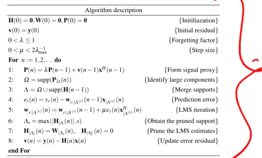
It was established in [58] that greedy algorithms can be converted into an adaptive mode, while maintaining their superior performance gains. We demonstrate below that this conversion is applicable in the multichannel set up. We focus our analysis on CoSaMP/SP due to their superior performance, but similar ideas are applicable to other greedy algorithms as well. Multichannel greedy algorithms can be approached via two strategies. The first approach assumes that the subsystems share the same sparsity pattern. Hence the greedy algorithm simultaneously recovers the support set (also known as joint sparsity or group sparsity) [12, 75] by choosing an element which reaches the maximum value of the multichannel energy. Under the second strategy adopted here, the subsystems exhibit different sparsity patterns [56]. Next greedy versions of the main adaptive multichannel algorithms are presented based on the CoSaMP/SP platform.

3.3.1 Greedy LMS filter

The multichannel adaptive greedy LMS algorithm modifies the proxy identification, estimation and error residual update. The error residual is evaluated by

v(n) =y(n)−H(n)x(n). (64) The above formula involves the current sample only, in contrast to the CoSaMP/SP scheme which requires all previous samples. A new proxy signal that is more suit-able for the adaptive mode, is defined as:

P(n) = n−1

∑

i=1 λn−1−i_v(i)xH_(i) and is updated by P(n) =λP(n−1) +v(n−1)xH(n)

This way the algorithm is capable of capturing variations on the support ofH. The estimateH(n)is updated by the LMS recursion [46, 70]. At each iteration the current regressorx(n)and the previous estimateH(n−1)are restricted to the instantaneous support originated from the support merging step. However, because the row support corresponding to each output is different, some extra care is required. Recall that any MIMO filter withnooutputs is simplified tonoMISO adaptive filters (all of

which have different row support). LetΛ denote the estimated set of indices and

Λ(r) _{(r=1,2, . . . ,n}

o) the set of indices associated with the rth row ofH(n). The

update equation for therth output is given by

h_r:|Λ(r)(n) =h_r:|Λ(r)(n−1) +µer(n)xH_|Λ(r)(n), ∀r=1, . . . ,no (65)

wherex_|Λ(r)(n)denotes the sub–vector corresponding to the index setΛ(r). If all rows ofHshare the same row support then the update step can be performed jointly