Developing methods of texture analysis in high resolution images of the Earth Philippe Maillard1
1
UFMG – Universidade Federal de Minas Gerais Av. Antônio Carlos, 6627 - Belo Horizonte – MG, Brasil
Abstract This paper presents the development and testing of two techniques of texture analysis based on different mathematical tools: the semi-variogram and the Fourier spectra. Three series of experiments are presented where these techniques are compared against a bench mark technique: the Grey-Tone Dependency Matrix. Results, their interpretation and conclusions are presented.
Keywords: texture analysis, semi-variogram, Fourier spectra, Bayes’theorem 1 Introduction
At high resolution, conceptual objects like forest or pasture usually show significant variations in their pixel values. Often stationary in nature, these variations can give rise to an apparent regular spatial pattern referred to as texture (Kittler, 1983). One of the key element that the interpreters use to identify, analyse and report was clearly the spatial arrangement of colour and tone that formed natural visual entities: visual texture (Haralick et al., 1973; Pratt et al., 1978).
Since there is no universally accepted definition of visual texture, one has to choose a definition that best reflects the objective or the results being sought. The definition chosen was given by Pratt (1991, p. 505): natural scenes containing semi-repetitive arrangements of pixels.
The principal objective of the research can be defined as follows: to investigate and compare major mathematical tools available for texture analysis and to implement and compare the most promising methods for texture segmentation / classification in digital images of the Earth. Within the context of this paper, the objective can be broken down in three goals:
− Goal n°1: To implement new tools, test and compare them against a more traditional approach. These tools should be computationally efficient and have some relation with psychophysical evidences about human visual texture perception.
− Goal n°2: To use these tools to understand better the mechanisms of texture recognition and to outline the most significant generic characteristics of texture without being tied to a particular method.
− Goal n°3: To outline and implement a systematic method for test and comparison of results obtained from different texture analysis method.
2 Current state of research
Recently, Reed and du Buf (1993) have made a extensive review of recent (since 1980) texture segmentation and feature extraction techniques. They claim that most development has been concentrated on feature extraction methods which seek to extract relevant textural information
Anais X SBSR, Foz do Iguaçu, 21-26 abril 2001, INPE, p. 1309-1319, Sessão Técnica Oral - Workshops
and map it onto a special dedicated channel called features. The authors classified the various
feature extraction methods as belonging to one of three possible classes: feature-based, model-based or structural. Cocquerez and Philipp (1995) have used a similar classification of image segmentation methods which they compare in various situations (including textured images).
In feature-based methods, some characteristics of texture (such as orientation, spatial frequency or contrast) are used to classify homogeneous regions in an image. Model-based methods rely on the hypothesis that an underlying process governs the arrangement of pixels (such as Markov chains or Fractals) and try to extract the parameters of such process. Structural methods assume that a texture can be expressed by the arrangement of some primitive element using a placement rule. Feature-based, model-based and hybrids methods have overwhelmingly dominated the scene in the last twenty years or so. One of their findings was that although so many different methods have been developed, no rigorous quantitative comparison of their results had ever been done. One possible reason for this situation lies in the mere fact that no strict methodology for performing such comparisons exists.
3 The development of two approaches to texture classification
Since Bela Julesz (1965) has shown evidence that human perception of texture could be modelled using second-order statistics (although he would later change his theory for the “texton” approach) many researchers have explored second-order statistics as possible features for texture analysis. Among the most common second-order statistics that have been used are the spatial-autocorrelation, the covariogram and the variogram. In particular, the semi-variogram has received much attention in the related field of Geostatistics (Clark 1979) and even directly applied to texture analysis (Woodcock et al. 1988; Ramstein and Raffy, 1989).
The frequency domain approach, also referred to as the Fourier Spectra approach, has been a long time favourite for texture analysis. From the early attempts at using it as a texture analysis tool by Rosenfeld (1962) to the recent use of Gabor functions in combination with it to create frequency- and orientation-specific texture features (e.g. Jain and Farrokhinia, 1991; Manjunath and Ma, 1996), the Fourier transform offers infinite possibilities not only for texture analysis but for applications requiring the analysis of spatial frequencies and their orientation. There is also some evidence that the Fourier transform is related to the way our perception of texture is processed by the visual cortex (Harvey and Gervais, 1978).
In order to evaluate a technique, it is necessary to have some comparison base. In this research, the comparison will take the form of another technique that has already been widely accepted by the scientific community and that, obviously performs reasonably well. Such method exists and was proposed by Haralick, Shanmugan and Dinstein (1973) who have named it Grey-Tone Spatial-Dependence Matrices. Not only do almost all the authors in visual texture analysis quote the GTDM but many have already used it as a comparison technique. Among them, Davis et al. (1979), Pratt (1991), Wu and Chen (1992) and Dikshit (1996) have either used the GDM method as a comparison or have described it in their review.
3.1The Variogram approach
After numerous tests using different ways to compute the variogram and transform it into texture features, the variogram approach was implemented the in following manner:
- For every pixel in the image, a neighbouring window (32 x 32 pixels) was considered.
- Four directional variograms (0°, 45°, 90° and 135°) were computed for all possible combinations in that window.
- The maximum lag size was equal to one half the window size.
- The semi-variogram was computed using its experimental form (Clark 1979):
( )
[
{
( ) (
)
}
2]
2 1 E * h = γγ x −γγ x+h γγ- Since the most important part of the variogram is usually its behaviour near the origin (Jupp
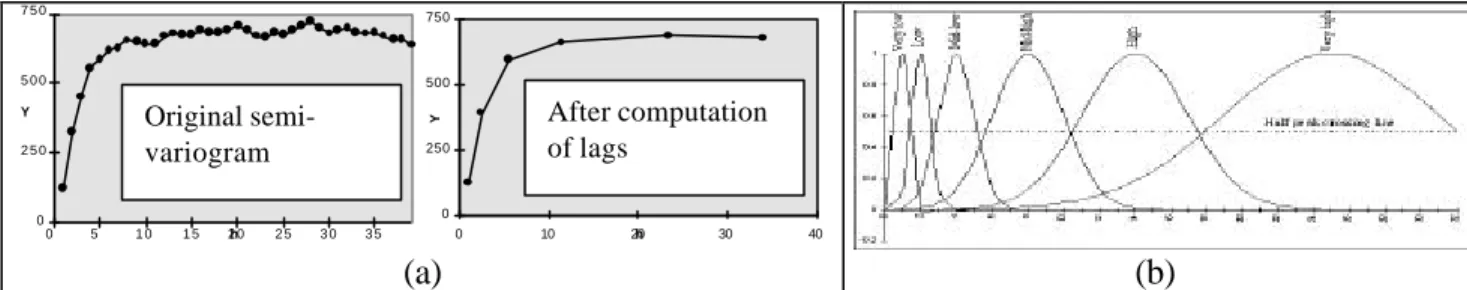
et al., 1989) six values (features) of the semi-variogram were computed according to the following semi logarithmic scheme: lag 1, lag 2, sum of lags 3 to 4, sum of lags 5 to 8, sum of lags 9 to 16 and sum of lags 17 to 32. Figure 1a illustrates the computation of these lags intervals. These values were computed for all four directions for a total of 24 features.
- The 24 directional features were then transformed to 18 rotation-invariant features: for each lag, the mean, standard deviation and sum of perpendicular ratios
(log[γγ0/γγ90+γγ90/γγ0+γγ45/γγ135+γγ135/γγ45]) was computed. 3.2The Fourier approach
In an effort to simplify the approach and to avoid a two-dimensional transform, the Fourier approach was implemented through appending all lines of pixels in the window in four directions (0°, 45°, 90° and 135°). This created artefact frequencies that were eliminated in a further step; the computation of the Fourier texture features can be summarised in the following manner: - For every pixel in the image, a neighbouring window (32 x 32 pixels) was considered. - Four directional transforms (0°, 45°, 90° and 135°) were computed for all appended lines. - Six Gaussian filters were applied to the transform to created the following texture frequency
features: very low (centred on 1 cycle per window of 32 or c/w), low (2 c/w), mid-low (4 c/w), mid-high (8 c/w), high (14 c/w), very high (25 c/w). Figure 1b illustrates these Gaussian filters. These values were computed for all four directions for a total of 24 directional features.
- The 24 directional features were then transformed to 18 rotation-invariant features: the mean,
standard deviation and sum of perpendicular ratios was computed for each frequency band.
0 2 5 0 5 0 0 7 5 0 0 5 1 0 1 5 2 0h 2 5 3 0 3 5 Y 0 250 500 750 0 10 20h 30 40 Y (a) (b)
Figure 1. The construction of texture features for the two main approaches to texture classification: a) the lag intervals of the semi-variogram, b) the Gaussian filters applied to the one-dimensional Fourier transform.
3.3The Grey-Tone Spatial-Dependence Matrices (Bench mark method)
The Grey-Tone Spatial-Dependence Matrices (GDM) method was implemented in similar Original
semi-variogram
After computation of lags
manner to its original form (Haralick et al., 1973). The measurements were chosen based on their success in a number of other studies (Davis et al., 1979; Sali and Wolfson, 1992; Wu and Chen, 1992 among others). The following summarises the implementation of the method:
- For every pixel in the image, a neighbouring window (32 x 32 pixels) was considered.
- Matrices were computed for three different lags (3, 6 and 12 based on the analysis of the variograms) and four directions (0°, 45°, 90° and 135°).
- Five measurements were computed for each matrix: contrast, angular second moment,
inverse difference moment, entropy and correlation for a total of 60 texture features.
- The 60 “directional” features were transformed into rotation-invariant features by computing the mean and standard deviation over the four original directions.
4 The experimental set up 4.1The test images
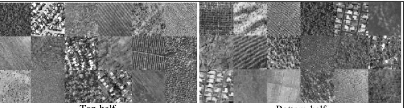
Many studies claim success rates for segmentation or classification of textures that are really dependent on the texture sample chosen for the experiments. This situation makes it difficult to perform any comparison between the results of these studies. To avoid this, only texture patches from real aerial photos were used in this research. The texture samples chosen are from six different generic classes: forest, residential areas, desert environment, agriculture, scrub and ocean waves. All were scanned at 450 dpi from 1:25000 black & white air photos giving an approximate resolution of 1.4 metre. All texture samples are presented in figure 2.
Top half Bottom half
Figure 2. The T36 texture set. The texture matrix is organised as six lines of six different textures. Each line contains an array of the six generic texture class; namely: forest, residential,
desert, crops, scrub and waves.
The first series of experiments was conducted on a small set of textures having great visual and geographical differences (the T6 set is formed by the first line of the top half of figure 2). The other experiments were implemented with the entire T36 set (figure 2) that has been constructed with a total of 36 texture samples from the same six generic classes but from different environmental conditions. This configuration bears various advantages:
• The first is that the initial set named T6, being small can easily and quickly be processed using the different methods and the results analysed for a meaningful comparison.
• The T36 texture set can easily be used in a variety of manners to infer the performance of the various techniques with respect to different experimental situations. The same set can be used to judge the amount of confusion at various levels like within groups (e.g. the group formed by the forest textures) and between groups (each of the row subsets).
• The T36 texture set has been arranged so that contiguous textures have little features in common so that texture edges are neatly defined to intentionally make the classification more difficult and to “challenge” the methods for texture edges situations.
4.2The comparison tool
Classification has been preferred over segmentation approaches for two main reasons:
- The decision rules of classification algorithm are simple and easy to control whereas many region-dependant segmentation algorithms use threshold that can be hard to set.
- The feature extraction phase enables a better analysis of the behaviour of the various textures for each method. These intermediary results can easily be analysed and described.
To avoid problems with the classifications, a number of considerations were taken:
1- Minimising Total Errors of Classification (TEC) is the best criterion. This is not, however, necessarily true since this does not consider the “cost” of every type of classification error. 2- In its normal form, the Bayes’rule assumes that all variables from the measurement vector
have a normal distribution. However, since the sample size is quite large (1024) and is the same for all textures, the assumption of normality can be relaxed (Scheffé, 1959).
3- TEC and its complement, Total Success of Classification (TSC) are acceptable ways to express the error measure through a contingency matrix. The Kappa statistics that considers the mere chance factor in the classification success (Jensen, 1996) will also be computed. 4- It is usually assumed when trying to perform a classification of an image that the conceptual
objects are homogeneous with respect to what is being classified. A quick glance at the texture patches reveals that this is not the case. Since it is the methods that are being tested rather than trying to achieve a real classification, this is an acceptable situation.
5- All a priori probabilities are equal since all texture samples are of equal size.
6- The edge effect has been considered by presenting unbiased results where the training areas and the edges and border areas have been removed from the statistics.
4.3Description of the experiments
Three series of experiments have been made, each aiming at different aspects of texture analysis. Experiment series #1: Separating a set of very different textures: evaluating the different approaches for separating and classifying a set of texture patches having very different visual characteristics and belonging to very different generic classes of objects with the T6 texture set.
Experiment series #2: Separating sets of similar textures: six subsets of the T36 texture set have been formed, each having six texture patches belonging to the same generic class. The objective is to assess the separation capability of the methods as well as their relative performance according to the textural context (e.g. forest vs residential).
Experiment series #3: Separating a mixture of both different and similar textures and testing the capacity of good association: testing the performance of each methods for the classification
of a large number of classes (36) belonging to both very similar and very different geographic realms. The experiment will also assess the good association capacity of all three methods. 5 Results and discussion
5.1First experiment: Separating a set of very different textures
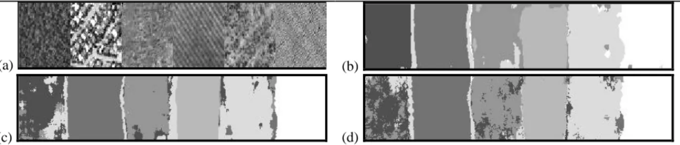
The first series of experiments has been organised in the following manner: first the grey-level dependency matrix method (GDM) will be applied to T6 then the variogram method (VGM) and finally the Fourier approach (FFT). In order to give more reliability to the results obtained with the T6 texture set, the classification tests were also performed on other five similar sets of six texture patches each. Figure 3 shows the graphical results of the best results obtained with the T6 set for each method while Table 1 show the tabular results of six sets of textures samples.
(a) (b)
(c) (d)
Figure 3. A graphical comparison of the best rotation-invariant classification results from all three methods: a) the initial T6 texture set, b) classification results from the GDM approach, c) the VGM approach and d) the FFT approach.
Texture set GDM Method
TSC (%) and (Kappa)
VGM Method
TSC (%) and (Kappa)
FFT Method
TSC (%) and (Kappa) Biased Unbiased Biased Unbiased Biased Unbiased
T6 91.41 (.897) 99.07 (.989) 85.00 (.820) 94.87 (.938) 83.56 (.803) 91.13 (.894) T6a 80.55 (.767) 94.07 (.929) 82.67 (.792) 95.29 (.943) 81.65 (.780) 95.85 (.950) T6b 82.62 (.791) 96.31 (.956) 80.56 (.767) 96.83 (.962) 80.52 (.766) 96.95 (.963) T6c 78.55 (.743) 94.15 (.930) 76.27 (.715) 94.26 (.931) 64.37 (.573) 86.21 (.834) T6d 75.97 (.712) 90.69 (.888) 71.45 (.657) 87.77 (.853) 72.91 (.675) 86.09 (.833) T6e 79.84 (.758) 94.10 (.929) 78.02 (.736) 96.29 (.956) 73.90 (.687) 91.21 (.895) Average 81.49 (.778) 94.71 (.937) 78.99 (.748) 94.22 (.931) 76.16 (.714) 91.24 (.895) Table 1. Classification scores (TSC and Kappa) from the classification of five textures sets. The sets all contained one sample of all the generic classes mentioned previously. The grey columns show the results without considering the borders, edges and training areas. The best results are in bold and the last line shows the average score .
The results clearly show that all three methods of texture analysis have very good potential for classification purposes since in all cases, the TSC obtained are well over 80%. However, given the slightly superior success rate of the GDM method, it has fail to demonstrate that the alternative methods proposed can bring any improvement to this traditional method. Although it is still early to draw conclusions, these first results suggest two thing about the GDM method:
(window size) is at the very heart of the GDM method and should be given proper importance as it can turn this somewhat traditional method a very powerful one.
2- The GDM method, when used properly, is perhaps the most efficient approach to simple texture classification problems where the texture characteristics are visually very different.
The second best method, the VGM approach, shows slightly poorer results with a difference in TSC of 6.5% with the T6 set (Kappa difference of ≈0.08) and about 2.5% for the average performance (all six sets). This difference cannot be attributed to mere chance and shows the superiority of the GDM approach for the classification of very different texture patches. Interestingly this gap falls significantly to a mere 0.5% with the unbiased results (eliminating borders and training areas) showing that the VGM method is more sensitive to edges.
The same reasoning can be applied to the FFT results which are comparable to the VGM ones with a difference in the best results of about 3% for both biased and unbiased results. The fact that in the frequency domain, the high frequencies (which correspond to small lags in the other methods) are usually regarded as noise can perhaps explain the poorer performance of the FFT method which is typically used to separate signal (larger frequencies) from noise.
5.2Second experiment: Separating sets of similar textures
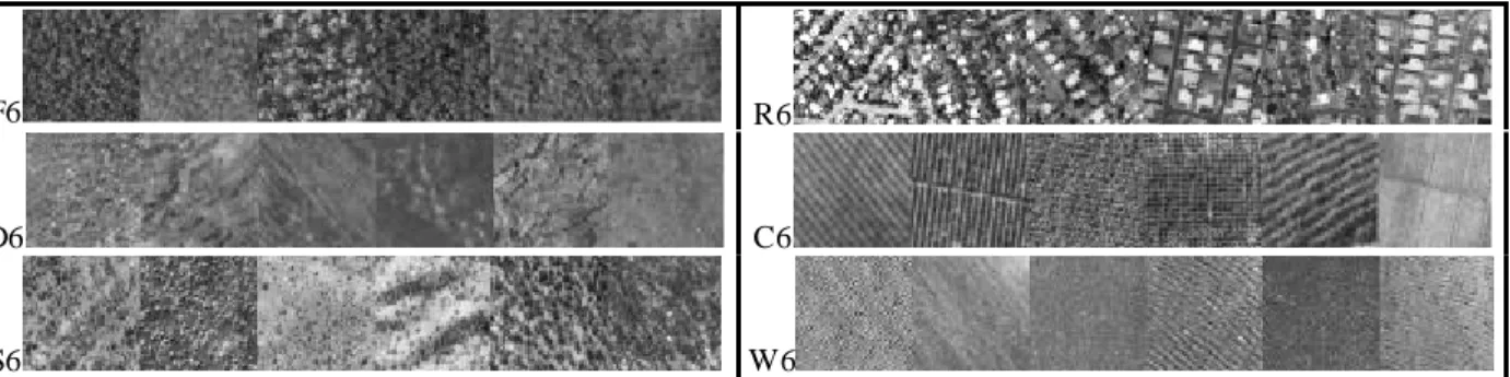
In the second series of experiments, six texture sets composed of similar texture samples were created (figure 4) in order to test the capacity of the three method to separate textures belonging to the same generic classes. Additionally, this series of experiments should enable to assess the characterisation of the particular aspects of texture that are more easily “graspable” by the three different methods.
F6 R6
D6 C6
S6 W6
Figure 4.. The six texture sets used to test the “separating” potential of the texture analysis methods. From top to bottom: Forest, Residential, Desert, Crops, Scrub and Waves.
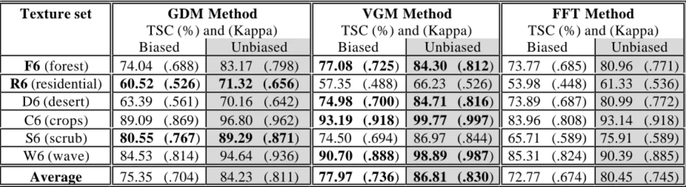
Table 2 shows the compiled results for all six texture sets both for biased and unbiased results. In four of the six texture sets, the VGM method performed better by yielding superior TSC scores of ≈3% (F6), ≈11%(D6), ≈4%(C6) and ≈5%(W6). Differences of ≈1%, ≈14% ≈3% and ≈4% are obtained when considering unbiased results. As for the other two cases (R6 and S6) the GDM method was superior by ≈3% and ≈6% respectively. In all cases, the VGM method was better than the FFT approach and only in one case was the FFT superior to the GDM method: D6. By all means, even when considering the latter exception, both the VGM and GDM methods proved more performing than the FFT by a margin of sometime over 10% in TSC score. The
difference between biased and unbiased results was not as clear as with the first experiments and, on average, the difference was of ≈9%, ≈11% and ≈8% for the GDM, VGM and FFT methods respectively.
The first texture set which proved the GDM superior is the Residential one which was also characterised by the lowest TSC scores of all six texture sets with values roughly between 54% and 60.5%. The first conclusion that this brings is that the R6 texture set is a poor candidate with ill-defined textures. The second more important observation is that the GDM method was probably superior because it includes other cues than simply variation over distance or spatial frequency in its feature set. In the second texture set for which the GDM had superior results, the S6 texture set, the situation is different but still keeps similar elements. Although the TSC scores are higher (roughly between 65% and 80%) a visual inspection of the individual texture patches reveal that most of them are poorly define or even have a dual textural characteristic (patch #3, #4 and #6 in particular) which tend to give more weight to cues other than the simple spacing of apparent objects on the background scene; a general superiority of the GDM method over the other two methods. This suggest that measurement type diversity can prove an important asset for textures that are not necessarily blessed with a homogeneous visual aspect.
As for the FFT method, its generally poorer performance can be attributed to two different facts. The first one is inherent to the approach that was chosen and that involved the appending of consecutive lines in a semi one-dimensional approach instead of the full fletched two-dimensional Fourier transform. The chosen approach might have created undesired artefacts. The second one is that, unlike real time series for which the Fourier transform was developed, spatial frequencies in these texture sets are ill-defined and often require a complex set of sine-like waves to described their square-like appearance.
Texture set GDM Method
TSC (%) and (Kappa)
VGM Method
TSC (%) and (Kappa)
FFT Method
TSC (%) and (Kappa) Biased Unbiased Biased Unbiased Biased Unbiased
F6 (forest) 74.04 (.688) 83.17 (.798) 77.08 (.725) 84.30 (.812) 73.77 (.685) 80.96 (.771) R6 (residential) 60.52 (.526) 71.32 (.656) 57.35 (.488) 66.23 (.526) 53.98 (.448) 61.33 (.536) D6 (desert) 63.39 (.561) 70.16 (.642) 74.98 (.700) 84.71 (.816) 73.89 (.687) 80.99 (.772) C6 (crops) 89.09 (.869) 96.80 (.962) 93.19 (.918) 99.77 (.997) 83.96 (.808) 93.14 (.918) S6 (scrub) 80.55 (.767) 89.29 (.871) 74.50 (.694) 86.97 (.844) 65.71 (.589) 75.91 (.589) W6 (wave) 84.53 (.814) 94.64 (.936) 90.70 (.888) 98.89 (.987) 85.31 (.824) 90.39 (.885) Average 75.35 (.704) 84.23 (.811) 77.97 (.736) 86.81 (.830) 72.77 (.674) 80.45 (.745) Table 2. Classification scores (TSC and Kappa) from the classification of the six textures sets each composed of texture patches belonging to the same generic class. The best results are in bold and the last line shows the average score.
5.3Third experiment: Separating a mixture of both different and similar textures
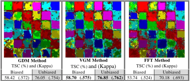
In the first phase of this experiment, the T36 texture set (figure 2) has been classified to assess the capacity for each method to deal with a complex situation where both very different and similar texture samples are mixed. In the second phase, a reclassification has been performed to assess the good association capability by observing the nature of the errors of the first phase: wether the wrongly classified pixels were at least within the good generic class.
The classification of the T36 texture set yielded results that are much poorer than what had been achieved in the other experiments. This was predicted to a certain extent since, by increasing greatly the number of classes, so does the probability of misclassification. Both the GDM and VGM methods produced results in the order of 58.5% for rotation-invariant feature sets. The FFT came in last with a TSC score approximately 5% lower. If these results are quite similar on the overall, the detailed analysis of their graphical correspondent shows that the behaviour of each method can be quite different (see table 3). The most striking difference lies in the size and frequency of wrongly classified pixels and in the patches they form. In the GDM results, these patches are relatively large, infrequent and generally concentrated around the edges of the texture patches. In the VGM classified image, these patches are smaller on the average but more frequent and sometime give a speckled impression. The square shape of the texture patches appear to be more respected in the VGM results. The classification result generated with the FFT feature set appear to suffer even more from the salt and pepper impression: the patches are mostly small but very frequent. These facts suggest various conclusions:
− The GDM method is the most stable of the three methods.
− The FFT and (to a lesser extent) VGM feature set are more likely to be affected by small variations in textures than the GDM approach.
− Texture edges are slightly better using the VGM approach.
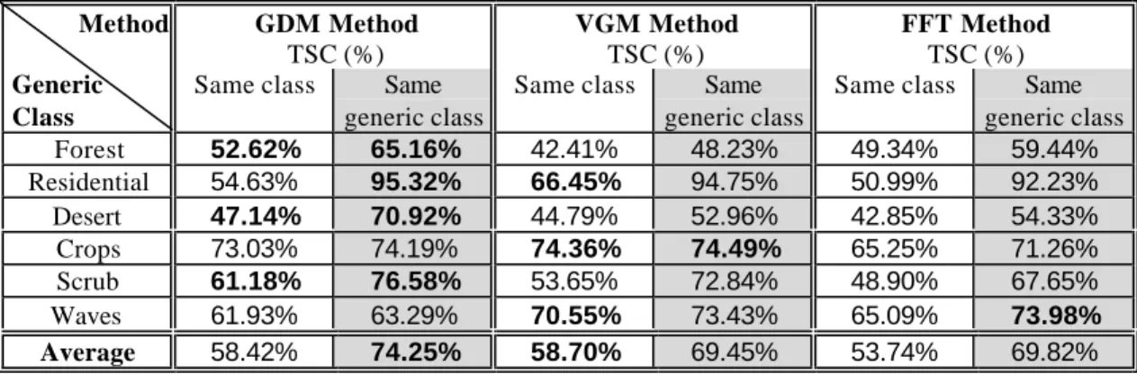
Although on the overall classification of the T36 texture set the VGM method scored best, it was this approach that benefited the least from the reclassification into generic classes moving from a TSC of 58.7% to 69.45%. Compared with the GDM method that went from 58.42% to 74.25 (table 7.46) or even the FFT whose TSC score went from 53.74% to 69.82%, these results tend to show that the VGM approach “sees” more differences between textures belonging to the same generic class than the other two methods.
GDM Method TSC (%) and (Kappa) VGM Method TSC (%) and (Kappa) FFT Method TSC (%) and (Kappa) Biased Unbiased Biased Unbiased Biased Unbiased 58.42 (.572) 76.05 (.754) 58.70 (.575) 76.85 (.762) 53.74 (.524) 70.18 (.693)
Table 3. Classification scores (TSC and Kappa) from the classification of the 36 textures set composed of six samples of each (six) generic class. The grey columns show the results without considering the borders, edges and training areas. The best results are in bold.
Method GDM Method TSC (%) VGM Method TSC (%) FFT Method TSC (%) Generic Class
Same class Same generic class
Same class Same generic class
Same class Same generic class Forest 52.62% 65.16% 42.41% 48.23% 49.34% 59.44% Residential 54.63% 95.32% 66.45% 94.75% 50.99% 92.23% Desert 47.14% 70.92% 44.79% 52.96% 42.85% 54.33% Crops 73.03% 74.19% 74.36% 74.49% 65.25% 71.26% Scrub 61.18% 76.58% 53.65% 72.84% 48.90% 67.65% Waves 61.93% 63.29% 70.55% 73.43% 65.09% 73.98% Average 58.42% 74.25% 58.70% 69.45% 53.74% 69.82%
Table 4. TSC scores of the good association analysis through the reclassification of the 36 textures set composed of six samples of each (six) generic class. The best results are in bold. 6 Conclusion
Three methods of texture classification have been tested in this paper, two of which have received a novel implementation: the semi-variogram and the Fourier spectra. Both have been implemented to be computationally efficient and related in some way to psychophysical evidences about the human vision. All three methods have proved to be powerful tools for texture classification but the grey-tone dependency matrix has shown superior results for dealing with simple situations where the textures are visually easily separable. The semi-variogram has, however proved superior for distinguishing very similar texture patches but has also proven more sensitive to the presence of borders and edges. In complex situations (large number of classes), the VGM and GDM have performed almost equally with generally poor results (but still beter than the FFT). The good association test proved the GDM method slightly superior.
Three goals have been set and, to some extent, reached: new implementations of mathematical tools for texture analysis were realised with success; insights on the behaviour of these tools for texture analysis has provided some understanding of the characteristics of texture that are difficult to classify; and a special use of classification using Bayes’theorem has proven an effective tool for testing and comparing the performance of texture analysis methods.
Other tests (complex textural situations and rotation-invariant properties) are also essential and are reported elsewhere (Maillard, 2000). Further studies will aim at testing these methods with other classifiers or segmentation schemes and in more realistic texture interpretation situations.
7 References
Clark, I. Practical Geostatistics. Applied Science Publisher, Essex, England, pp. 1-41, 1979. Cocquerez, J.P. and Philipp, S. (Eds.) Analyse d’Images: filtrage et Segmentation. Masson,
Paris, 1995.
Davis, L.S., Johns, S.A. and Aggarwal, J.K. Texture analysis using generalized co-occurrence matrices. IEEE Trans. on Pattern Analysis and Machine Intelligence, vol. PAMI-1, no. 3, 1979, pp. 251-259.
Dikshit, O. Textural classification for ecological research using ATM images. International Journal of Remote Sensing, vol. 17, no. 5, 1996, pp. 887-915.
Haralick, R.M., Shanmugan, K. and Dinstein, I. Texture feature for image classification. IEEE Trans. Systems, Man and Cybernetics, SMC-3, 1973, pp. 610-621.
Harvey, L.O.Jr. and Gervais, M.J. Visual texture perception and fourier analysis. Perception & Psychophysics, vol. 24, no. 6, 1978, pp. 534-542.
Jain, A.K. and Farrokhnia, F. Unsupervised texture segmentation using Gabor filters. Pattern Recognition, vol. 24, no. 12, 1991, pp. 1167-1186.
Jensen, J.R. Introductory digital image processing – A remote sensing perspective, Prentice Hall, New Jersey, 1996.
Julesz, B. Texture and visual perception. Scientific American, vol. 212, 1965, pp. 38-48.
Jupp, D.L.B., Strahler, A.H. and Woodcock, C.E. Autocorrelation and regularization in digital images. II. Simple image models. IEEE Trans. on Geoscience and Remote Sensing, vol. 27, 1989, pp. 247-258.
Kittler, J. Image processing for remote sensing, Philantropical Transactions of the Royal Society of London, vol. A 309, 1983, pp. 323-335.
Maillard, P. Texture in High Resolution Digital Images of the Earth, Ph.D. Thesis, University of Queensland, Qld, Australia, 2000.
Manjunath, B.S. and Ma, W.Y. Texture features for browsing and retrieval of image data, IEEE Trans. on Pattern Analysis and Machine Intelligence, vol. 18, no. 8, 1996, pp. 837-842. Pratt, W.K. Digital Image Processing, John Wiley & Sons, New York, second edition, 1991. Pratt, W.K., Faugeras, O.D., Gagalowicz, A. Visual discrimination of stochastic texture fields.
IEEE Trans. on Systems, Man and Cybernetics, vol. SMC-8, no. 11, 1978, pp. 796-804. Ramstein, G. and Raffy, M. Analysis of the structure of radiometric remotly-sensed images.
International Journal of Remote Sensing, vol. 10, no. 6, 1989, pp. 1049-1073.
Reed, T.R. and du Buf, H. A review of recent texture segmentation and feature extraction techniques, CVGIP: Image Understanding, vol. 57, no. 3, 1993, pp. 359-372.
Rosenfeld, A. Automatic recognition of basic terrain types from aerial photographs. Photogrammetric Engineering, vol. 28, no. 1, 1962, pp 115-132.
Sali, E. and Wolfson, H. Texture classification in aerial photographs and satellite data. International Journal of Remote Sensing, vol. 13, no. 18, 1992, pp. 3395-3408.
Scheffé, S. The Analysis of Variance, Wiley, New York, 1959.
Woodcock, C.E., Strahler, A.H. and Jupp, D.L.B. The use of variogram in remote sensing and simulated image: II. Real digital images. Remote Sensing of Environment, vol. 25, 1988B, pp. 349-379.
Wu, C.-M. and Chen, Y.-C. Statistical feature matrix for texture analysis. CVGIP: Graphical Models and Image Processing, vol. 54, no. 5, 1992, pp. 407-419.