Original Article
Estimation of regression
quantiles in complex surveys
with data missing at random:
An application to birthweight
determinants
Marco Geraci
Abstract
The estimation of population parameters using complex survey data requires careful statistical modelling to account for the design features. This is further complicated by unit and item nonresponse for which a number of methods have been developed in order to reduce estimation bias. In this paper, we address some issues that arise when the target of the inference (i.e. the analysis model or model of interest) is the conditional quantile of a continuous outcome. Survey design variables are duly included in the analysis and a bootstrap variance estimation approach is proposed. Missing data are multiply imputed by means of chained equations. In particular, imputation of continuous variables is based on their empirical distribution, conditional on all other variables in the analysis. This method preserves the distributional relationships in the data, including conditional skewness and kurtosis, and successfully handles bounded outcomes. Our motivating study concerns the analysis of birthweight determinants in a large UK-based cohort of
children. A novel finding on the parental conflict theory is reported. R code implementing these
procedures is provided.
Keywords
chained equations, Khmaladze tests, multiple imputation, paediatrics, weights
1
Introduction
This paper offers general guidance for conducting quantile regression (QR) analysis of complex survey data. We start considering the case in which regression quantiles are estimated from a sample of observations taken from a finite population using a complex design. We then consider estimation issues that arise when several variables of interest are partially observed. Our motivating example is a study of determinants of birthweight in children of the UK Millennium Cohort Study (MCS), a longitudinal survey of British children born at the beginning of the 21st century.1
Centre for Paediatric Epidemiology and Biostatistics, Institute of Child Health, University College London, UK Corresponding author:
Marco Geraci, Centre for Paediatric Epidemiology and Biostatistics, Institute of Child Health, University College London, 30 Guilford Street, London WC1N 1EH, UK.
Email: [email protected]
Statistical Methods in Medical Research 0(0) 1–29
!The Author(s) 2013 Reprints and permissions:
sagepub.co.uk/journalsPermissions.nav DOI: 10.1177/0962280213484401 smm.sagepub.com
Conditional quantiles for continuous response variables2have a long history in econometrics and they have been applied in many other research fields.3Their ability to model the location, scale and shape of the observed distribution of the response variable conditional on a set of predictors offers the opportunity to investigate a wide range of effects that location-shift models are unable to handle. In addition, QR is inherently robust to outliers in the outcome and mathematically flexible in handling transformations of the response variable that can be exploited for a variety of purposes.4–7 In contrast, ordinary least squares methods can overshadow important associations between the predictors and the outcome distribution.
There are a number of models for conditional quantiles which, in a sense, mirror regression models that have been developed for the estimation of the location parameter, including parametric, nonparametric8–10 and semiparametric11 models, linear and nonlinear models and models for discrete4,12 and survival data.13 An overview of QR inferential and computational issues is given in Koenker’s monograph.14
The number of applications of QR in medicine has increased in recent years. In particular, QR has been applied in paediatric research where both methodological and applied studies have led to improvements on several fronts, including the understanding of birthweight determinants,15–19child growth and obesity,20–24malnutrition,25cancer aetiology26and hypertension,27where the common denominator is the analysis of the tails of distributions of variables strongly associated with adverse health risks (e.g. birthweight and blood pressure).
The data used in these studies generally come from hospital registrations and national healthcare systems data collections. However, data from population-based multi-purpose surveys are another important source of information since they provide details on health and socioeconomic conditions of children, their families and the environment in which they live. Moreover, longitudinal surveys allow exploring the impact of early life exposures on long-term health outcomes from a life course perspective.
The analysis of survey data involves the estimation of population parameters and related measures of uncertainty by using models that handle design features such as probability sampling weights, stratification and cluster sampling. Accounting for unequal inclusion probabilities is necessary in order to obtain consistent estimates. A number of methodological advances have been made in the development of multivariable models for correlational studies including linear, logistic and probit regression models, survival analysis models and structural equation models.28 The estimation of finite population quantiles has attracted much attention in the literature of survey analysis29–32 and, recently, a general asymptotic theory for nondifferentiable survey estimators, including sample quantile estimators, has been proposed.33 In general, there are few applications of QR in studies based on complex survey data.34,35
Inference for survey estimators is further complicated by nonresponse, a common problem in survey studies. This can affect all items of the survey for units who do not respond or refuse to participate in an interview (unit nonresponse), although some information for those units is typically available prior to interview and can be used for nonresponse adjustments; or it can involve only certain items due to early drop-out from the study, or questionnaire items filled with ‘don’t know’ or ‘refused’ (item nonresponse).36 The reduction of available information that follows from nonresponse has effects of varying gravity, depending on the type and degree of missingness. The much-celebrated Little and Rubin’s classification of missing data37 clarifies the conditions under which inference can lead to estimation bias if the missing process is not taken into account. In particular, missing at random (MAR) assumptions are often introduced and their tenability may be sustained by sensible modelling choices. MAR mechanisms can be thought as a middle-way between missing completely at random (MCAR) and missing not at random (MNAR) mechanisms.
Here, we consider a multiple imputation (MI) strategy based on sequential conditional regressions as opposed to joint modelling.38 The former approach avoids specifying a joint distribution for the imputation model by using a sequence of conditional specifications for each variable whose missing values are to be imputed. This strategy is advantageous when several variables, continuous and discrete, are included in the analysis model. In particular, missing values of continuous variables are imputed using conditional quantile models.39 A distribution-free imputation procedure based on nonparametric kernel regression to estimate the distribution function and quantiles of an incomplete response variable under MAR assumptions has been developed.40Other approaches to apply QR in the presence of missing data have been proposed.41–43 The rest of the paper is organized as follows. In Section 2, we describe the MCS data and the sampling design. In Section 3, we introduce the model of interest and related methods of analysis, including a complete case analysis of the MCS birthweight determinants. We then present an imputation procedure for when nonmonotone missingness affects both continuous and discrete variables, followed by a simulation study to assess the imputation models (Section 4). We conclude with an MI analysis of the MCS birthweight determinants (Section 5) and final remarks (Section 6).
The code to run the simulation study and the MCS analyses was written inR44and the following packages were used: survey,45,46 quantreg47 and mice.48 Additional R code for custom-defined functions to implement the methods proposed in this paper is provided in Appendix B.
2
The data
The MCS is a longitudinal study of a cohort of UK children born between September 2000 and January 2002.1Here, we provide a background on its sampling design and briefly describe the data selected for the analysis.
The survey population was defined as all children alive and living in the UK at age 9 months and eligible to receive Child Benefit at that age49(all UK residents qualify for Child Benefit if they have children younger than 16 years). Details on the sampling population resulted from exclusion of children who died before 9 months of age is given by Cullis.50The population was stratified by UK country and, in order to adequately represent disadvantaged and ethnic minority children, stratification by these variables within country was carried out using data available at the electoral ward level.49 In particular, population in England was stratified by: ‘ethnic’, children living in wards that, in the 1991 Census of Population, had an ethnic minority population of at least 30% of the total; ‘disadvantaged’, children living in wards other than ‘ethnic’ which fell into the upper quartile of the ward-based Child Poverty Index (i.e. poorest 25%) for England and Wales; and ‘advantaged’, children not living in wards classified as ‘ethnic’ or ‘disadvantaged’. Wales, Scotland and Northern Ireland populations were stratified by ‘disadvantaged’ and ‘advantaged’ wards.
Families were taken from a random sample of electoral wards, the primary sampling unit (PSU), disproportionately stratified to ensure an adequate representation of disadvantaged areas and ethnic minority groups. Details on the calculation of sampling weights and adjustment for unit nonresponse are given by Plewis.49,51
Parents/guardians of the children were interviewed when the children were aged nine months, three, five and seven years. We abstracted data from the first sweep of the survey on birthweight, gestational age and sex of singletons for whom the main respondent at the interview and the respondent’s partner were the natural parents. This gave information for 15,070 children, with the main respondent being the mother in 15,060 cases. Additional information for the mothers
comprised reported weight before pregnancy, reported height, age at delivery, parity, highest
educational degree attained (including GCSE, A-level/Diploma and academic), tobacco
consumption habits before, during and after pregnancy, marital status, ethnicity, antenatal care received and diabetes status. Reported weight and height of children’s natural fathers were also included. Some of the questionnaire items that were missing at the first sweep were retrieved from either the second or the third sweep if available.
A summary of the dataset, including the number of missing values, is given in Table 1. The number of incomplete cases (i.e. with at least one missing item) was 3066, 20% of the sample. Paternal weight had the highest proportion of missing data (15%). For this variable and for maternal weight, we replaced 30 outliers with missing values (more details in Section 5.4).
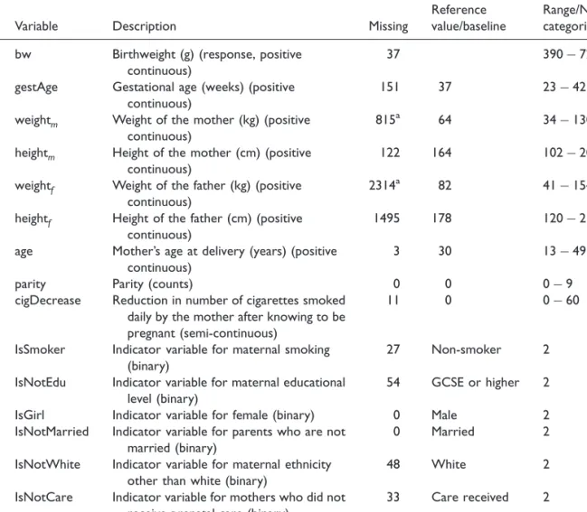
Table 1. Details of variables included in the analysis for 15,070 MCS children.
No. Variable Description Missing
Reference value/baseline
Range/No. categories 1 bw Birthweight (g) (response, positive
continuous)
37 3907230
2 gestAge Gestational age (weeks) (positive continuous)
151 37 2342
3 weightm Weight of the mother (kg) (positive continuous)
815a 64 34130
4 heightm Height of the mother (cm) (positive continuous)
122 164 102206
5 weightf Weight of the father (kg) (positive continuous)
2314a 82 41154
6 heightf Height of the father (cm) (positive continuous)
1495 178 120213
7 age Mother’s age at delivery (years) (positive continuous)
3 30 1349
8 parity Parity (counts) 0 0 09
9 cigDecrease Reduction in number of cigarettes smoked daily by the mother after knowing to be pregnant (semi-continuous)
11 0 060
10 IsSmoker Indicator variable for maternal smoking (binary)
27 Non-smoker 2
11 IsNotEdu Indicator variable for maternal educational level (binary)
54 GCSE or higher 2
12 IsGirl Indicator variable for female (binary) 0 Male 2
13 IsNotMarried Indicator variable for parents who are not married (binary)
0 Married 2
14 IsNotWhite Indicator variable for maternal ethnicity other than white (binary)
48 White 2
15 IsNotCare Indicator variable for mothers who did not receive prenatal care (binary)
33 Care received 2 16 IsDiabetic Indicator variable for maternal diabetes
status (binary)
8 Non-diabetic 2
Reference values or baselines and variable range or number of categories are detailed as they will be used in subsequent analyses.
2.1
Survey weights and finite population correction
We now provide a brief note on additional sampling details. MCS sampling weights were calculated proportionally to the fraction of electoral wards selected by systematic sampling of the population wards ordered by size within strata. Although an implicit stratification by region and ward size was introduced, this had a marginal design effect.49It follows that children in the same stratum received the same weight. Also, a second set of survey weights was calculated to adjust for unit nonresponse in the issued sample. Unit nonresponse is a source of concern in this specific case. In fact, we might expect that children with very low birthweights are not well represented in the MCS sample (e.g. parents refused to participate as their child was receiving postnatal care) and, thus, that a MNAR mechanism is at play. Also, infant mortality before 9 months of age50 may have introduced additional upward bias in the left tail of the distribution. An approximate calculation based on population birthweight data (further details available upon request) suggests that only 56% of the low birthweights not represented in the MCS sample may be accounted for by infants who died before becoming eligible for the survey.
Unless explicitly stated, we will make use of sampling weights adjusted for unit nonresponse in all subsequent analyses of the MCS data.
3
QR in complex surveys
3.1
Population model
Initially, we focus on the population model, assuming that all units have been completely observed. Letðy,X,FÞbe the data for a sample of sizentaken from a population of sizeN, whereydenotes an
n1 continuous response variable, X denotes a nq set of predictors with row vectors x0i,
i¼1,. . .,n and F collects sampling design variables. Also, let FyjX,F denote the unknown
cumulative distribution function of y given ðX,FÞ. Our inferential target is the population conditional quantile function QyjX,F Fyj1X,F. That is, we want to make a statement about
specific quantiles of the distribution of y conditional on predictorsXand designF. Matrices will be denoted with upper case bold letters (e.g.U), while column and row vectors with lower case bold letters (e.g. u and u0). Depending on the context, the symbol will be used interchangeably to
indicate ‘distributed as’, ‘approximately equal to’ or as response-covariate separator in a linear model formula (e.g.yx).
We will only consider the case in whichF defines a stratified clustered design since this represents the design that motivated our study. Leth¼1,. . .,Hindex population fixed strata and letmhbe the size of a sample of clusters (e.g. counties or electoral wards) randomly selected within stratum h
(these also represent PSUs in our modelling). Survey weights are introduced to account for selection probability and, possibly, unit nonresponse. The following developments can be easily extended to account for other designs.
Suppose that the sample ðy,XÞ was obtained under simple random sampling (SRS) without replacement from a largeNandnN(i.e. sampling fraction very small) and that we wanted to fit thep-th conditional quantile function
where bð Þp is a q1 vector of regression coefficients indexed by p. If we ignore the unequal sampling probability, the p-th regression quantile bð Þp could be the estimated by minimizing the loss function2 Xn i¼1 p yix0ib ð3:2Þ
with respect tob, where pð Þ ¼s s pIðs50Þ
ands2R, and the standard inferential theory for regression quantiles could be applied with some approximation. See Chatterjee32 for a recent overview of inferential issues related to marginal quantiles estimated from samples in finite populations.
With data obtained from designs more complex than SRS, the estimation of population statistics and their uncertainty measures needs to take into account the design. Stratification and clustering can in principle be adjusted for by including the relevant sampling variables in the linear predictor. Generalized linear mixed models, for example, allow modelling the intra-class correlation due to survey clustering by means of random effects. Alternatively, cluster-specific parameters can be entered as fixed effects though care must be taken in controlling for standard error inflation through some form of parameter shrinkage. QR methods for repeated and clustered data have been proposed,52–54 although models for complex hierarchical structures (e.g. more than two levels of nesting or cross-classified multilevel models) are yet to be developed. In general, dealing with survey weights in hierarchical models can be challenging.28
Weighting in survey estimators is used to account for unequal inclusion probabilities assigned to sample observations. In a QR context, we consider the following weighted loss function:
Xn
i¼1
wip yix0ib
, ð3:3Þ
wherewiare survey weights possibly adjusted for unit nonresponse.
The unknown regression coefficientbin (3.2) and (3.3) can be estimated, for example, using
well-developed linear programming algorithms47 or gradient search methods,55 which are
computationally fast. The former include classical simplex methods, suitable for problems of small to moderate size, and interior-point methods, such as Frisch–Newton algorithms,56 recommended for large problems. As opposed to least squares estimators, quantile estimators involve nondifferentiable functions of the quantities to be estimated. The usual Taylor linearization used to obtain an approximate estimate of the variance of survey estimators cannot therefore be applied. A practical way to overcome this computational issue is to use bootstrap estimation. In Appendix A, we briefly describe the method proposed by Canty and Davison.57–59 We also discuss preliminary results using Wang and Opsomer’s33approach.
Details on how to fit QR models by minimizing (3.3) and estimate bootstrap standard errors inR
are given in Appendix B. The application of these methods using the MCS data is described in the following section.
3.2
Birthweight determinants
Birthweight has long been recognized as an important surrogate for infant well-being. In particular, birthweight is a strong predictor of infant mortality and morbidity and thus provides a well-established base for clinical indicators. Least squares methods are commonly used in birthweight
analyses to assess the effects of determinants such as maternal health-related lifestyle habits (e.g. smoking and diet) and environmental factors (e.g. pollution). Mean regression, however, is generally unable to reveal effects of these determinants on the tails of the distribution which are of particular interest since small and macrosomic babies are at increased risk of morbidity and mortality. At the population level, studies in different countries show that birthweight follows approximately a normal distribution with an elongated left tail. The latter is mostly explained by preterm babies who tend to weigh less than babies born after 37 weeks of gestation. However, even at the population level, conditional birthweight distributions may be far from normal and distributional effects may be more complex than those explained by location-shift models.
Early QR analyses of population birthweight can be found in Abrevaya15 and Koenker and Hallock60 who analysed birthweights for about 200,000 US babies from the Detailed Natality Data (National Center for Health Statistics). In their analyses, the QR estimates associated with factors such as maternal smoking, age and weight gain were not constant across the conditional birthweight distribution, suggesting that these predictors may exert complex distributional effects. Cases with missing data were excluded. See also Chernozhukov and Ferna´ndez-Val61 for an interesting application of extremal QR (i.e. very low and very high quantiles) and Abrevaya and Dahl16 for the analysis of panel data on maternally linked births which takes into account unobserved characteristics of the mothers.
We are interested in estimating the quantiles of MCS birthweights conditional on determinants listed in Table 1. Here, we follow a conditional approach for gestational age mindful that the latter is a potential mediator of other effects. Joint modelling approaches to birthweight and gestational age have been proposed.62Figure 1 provides a breakdown of the birthweight histogram by gestational age. As expected, the distribution is shifted to the left for preterm infants (537 weeks) and departs from normality. Figure 1 also shows the histogram of gestational age, whose distribution is highly asymmetric and leptokurtic.
bw Density 0 2000 4000 6000 8000 0e+00 2e−04 4e−04 6e−04 8e−04 gestAge Density 20 25 30 35 40 45 0.00 0.05 0.10 0.15 0.20 0.25
Figure 1. Left: histogram of birthweight. Children born at 37 weeks or later (white) and children born before term (grey) are contrasted. Right: histogram of gestational age.
We now proceed with a complete case analysis using the methods described in Section 3.1, under MCAR assumptions. After excluding partially observed units, there were 12,004 observations available for the analysis. The quantiles p¼0:05 andp¼0:01 of the observed birthweights were equal to, respectively, 2410 and 1626 g, approximately corresponding to standard thresholds for low (52500 g) and very low (51500 g) birthweight.
All continuous predictors were centred at their mean value, with the exception of gestational age which was centred at 37 weeks. Moreover, parental weight and height were divided by their standard deviation (internal standardization) to obtainz-scores. These scores were further reparametrized as in Griffiths et al.63 to study the effects of differential parental weight and height contributions on birthweight, namely the effect of the half difference ðw=hÞeighthd¼ ðw=hÞeight m ðw=hÞeightf=2 and the independent effect of the mean (i.e. sum)ðw=hÞeightsum¼ ðw=hÞeightmþ ðw=hÞeightf.
We considered the following QR model:
Q pð Þ ¼0ð Þ þp 1ð ÞgestAgep þ2ð Þweightp hdþ3ð Þweightp sumþ4ð Þheightp hd
þ5ð Þheightp sumþ6ð Þagep þ7ð Þparityp þ8ð ÞðcigDecreaseÞ þp 9ð ÞIsSmokerp
þ10ð ÞIsNotEdup þ11ð ÞIsGirlp þ12ð ÞIsNotMarriedp þ13ð ÞIsNotWhitep þ14ð ÞIsNotCarep þ15ð ÞIsDiabetic:p
ð3:4Þ
The intercept 0ð Þp can be interpreted as the birthweight p-th quantile for male children born at 37 weeks gestation from: married parents whose difference/mean weight/heightz-scores are zero; 30-year-old, white, non-diabetic, zero-parity mothers with GCSE educational level or higher, who are non-smokers and who received prenatal care.
A sequence of 21 regression quantiles,p2f0:01, 0:05, 0:1,. . ., 0:9, 0:95, 0:99g, was then obtained using the methods illustrated in Section 3.1. In particular, the loss function (3.3) was weighted using MCS sampling weights. Since sampling fractions were as high as 18% due to oversampling, variance estimates were adjusted with a finite population correction. A bootstrap sample sizenB¼100 was used to estimate the variance of the regression quantiles.
Table 4 shows point estimates and standard errors for selected quantiles (results for all quantiles are available upon request). A discussion of the results is deferred to Section 5.
4
QR and missing data
4.1
Missing data modelling
Our estimand of interest is, again, a model of the type (3.1). However, we assume thatyandXare not fully observed. Now let ðy,X,F,RÞ be the data and define the augmented nðqþ1Þ matrix Z¼ðy,XÞ, with column vectorsz1,. . .,zqþ1. The missing indicator matrixRcontains nonresponse information for Zand has columns r1,. . .,rqþ1 whose elements ri,j,i¼1,. . .,n, j¼1,. . .,qþ1, take the value 1 when the corresponding itemzi,jis observed and 0 otherwise. Letnjandnj¼nnj denote the number of observed and missing values inzj, respectively, and letAjbe the set indexing the units i for which ri,j¼0. In addition, let obs and mis denote restriction of variables to their
observed and missing parts, respectively. Under MAR assumptions, the distribution of R
conditional onZobs is independent ofZmis
PrðRjZobs,Zmis,Þ ¼PrðRjZobs,Þ, ð4:1Þ
Let Zj denote Z without the j-th column and ¼ 01,. . .,q0þ1
0
be a partitioned parameter vector, distinct fromn. Without loss of generality, suppose for the moment thatZj is completely observed. Equation (4.1) implies that, conditionally onZj, the distribution of the variablezjis the same among the cases for whichzj is observed as it is among the cases for which zj is missing,64 that is Fobs zjZj,F,j ¼Fmis zjZj,F,j , ð4:2Þ
which corresponds to the assumption of ignorability.65This identity allows us to use the conditional distribution function of respondents to draw independent samples to be imputed toZmis. The MAR assumption provides the basis for a consistent estimation of the conditional distribution. Conditioning the probability model on the sampling design is considered in order to avoid potential imputation bias.66
Here, we adopt a fully conditional specification (FCS) in contrast to joint modelling. For an overview and discussion of these two approaches to MI, see Van Buuren38and references therein. The following three stages for QR estimation are considered:
(a) Drawmsamples independently using, in turn, sequential conditional modelsFobs zjZj,F,j
for all variableszjwith missing values. Since in general the predictorsZjmay be incomplete, a preliminary imputation of all missing values is carried out by SRS with replacement from the observed values.67The preliminary imputed values are then updated with the most recent draws from the sequential conditional models. The process may be repeated several iterations in order to stabilize the results.67
(b) Analyse each imputed dataset yk,Xk,F, k¼1,. . .,m, using an appropriate QR model
QyjX,Fð Þp to obtainbbkð Þp and its standard error seðbbkðpÞÞ. The latter can be calculated, for example, using a bootstrap approach (see Appendix A for more details).
(c) Pool themestimatesbbkð Þp and seðbkðpÞÞusing Rubin’s rules.
The preliminary imputation of Zj in step (a) is based on the assumption that units are exchangeable and such assumption is commonly violated in complex surveys. In the case of a stratified clustered sample, the preliminary imputation step could ideally be made more efficient by conditioning the sampling on stratification as well as clustering variables, provided that the number of observations available is sufficient for this purpose.
In the next two sections, we illustrate an imputation modelling approach to mixed (i.e. continuous and categorical) data which assumes a generalized missing pattern and takes the sampling design into account. Initially, we focus on continuous variables only; then, we briefly consider models for categorical variables.
4.2
Imputation models for continuous variables
Much of the literature on MI is dedicated to location models. A linear regression model (i.e. normal) is usually assumed for continuous data, whereas logistic, multinomial or log-linear models are used to impute categorical variables. The assumption that all the information is contained in the location parameter might, however, be too restrictive and lead to estimation bias associated with an inadequately chosen imputation model. In specific situations, distributional features like
heteroscedasticity and skewness can be accommodated by simple monotonic transformations. A general approach to handle conditional distributions that exhibit complex relationships with the model predictors is necessary when simpler strategies do not apply.
Some methods that deal with skewed continuous variables are described by White et al.,67 including shifted-log and (marginal) Box–Cox transformations (BCT). Because of their inability to remove non-normal features other than skewness, such transformations cannot be generally qualified as methods for non-normal distributions. Moreover, they require estimation of unknown parameters from the observed data, in addition to the imputation model’s parameters. In particular, White et al. suggested that if BCTs are applied to marginal rather than conditional distributions, this may not be relevant for the analysis. However, no formal discussion on this topic was provided.
Predictive mean matching68 (PMM) is an ad hoc method that can be used effectively for imputation. Observed values whose predicted mean are closest to the predicted mean for the missing value are elected as ‘donors’ and a value taken randomly from the set of donors is imputed. In Schenker et al.,69 partially parametric approaches to MI were compared to normal imputation. In particular, PMM and a modified PMM (local residual draw) were shown to be robust to model miss-specification and different (symmetric) error distributions. However, PMM requires a sufficient number of ‘donors’ from where to sample the values to be imputed. An interesting approach based on transformations of the target variable is described by He et al.,70 where the Tukey’s gh distribution is applied to accommodate for skewness and tail elongation in MI. This transformation was shown to be preferable to a log-transformation to reduce skewness. As in the case of BCT, the gh transformation requires estimating unknown parameters and a bootstrap approach was suggested. These methods69,70 were explored in an MCAR framework. BCTs are also considered by Raghunathan et al.71 for sequential regression multivariate imputation (SRMI) based on Metropolis–Hastings sampling. These authors warned about the computational burden of SRMI in analyses of large data sets with many variables, which are typical in survey studies.
To overcome some of the limitations of the methods mentioned above, we build an MI procedure starting from a distribution-free approach based on conditional quantile estimation proposed by Bottai and Zhen39 in the context of SRS. Their approach exploits the well-known probability integral transformation theorem which is used in pseudo-random numbers generation: if vF
and uUnif 0, 1ð Þ, then F1ð Þ u F, that is v and F1ð Þu have the same distribution. This theorem and equation (4.2) provide our sampling framework for imputation. We apply it to continuous variables only although, in principle, extensions to discrete variables can be considered (see next section).
The aim is to imputenj missing values of a partially observed continuous variablezjwithin the FCS algorithm described in the previous section. A common imputation model for continuous responses is the iid linear model zi,j¼Zjþi, with i N 0,2
and i2Aj. However, this location-shift model may be too restrictive in some situations. We therefore consider a distribution-free approach to sample from FzjjZj,F, the distribution function ofzj conditional on
ZjandF:
(i) Obtain a sample u of size nj independently from a standard uniform distribution. To avoid sampling in the vicinity of the boundaries which could cause computational inconveniences in step (ii), we can restrict the sampling domain to Unifð!, 1!Þ with! sufficiently small, say !¼0:001. The parameter!, as we shall see in the MCS birthweight analysis, can be used to trim or truncate the distribution ofzi,j.
(ii) Estimate the QR model
QzjjZj,Fð Þ ¼ui Zjð Þui ð4:3Þ
for each quantileui,i2Aj. (iii) Obtain and impute the valuez
i,j¼Zjbcð Þ,ui i2Aj.
Suppose we fix!¼0:001 in step (i). The uniform values u can be grouped into small intervals
between 0.001 and 0.999 (for a maximum number of 207 breakpoints, i.e.
u2f0:001, 0:002,. . ., 0:005, 0:01,. . ., 0:995, 0:996, . . ., 0:999g) to reduce the number of quantiles that are too close one to each other and for which estimates would not differ substantially. Alternatively, rather than with pre-defined quantile breakpoints, a possibly more efficient computation could be obtained by estimating the conditional quantile function with a number of breakpoints determined by changes of solution. The latter, however, has been shown to grow withn.72
There are several advantages with a quantile-based imputation. Provided that the conditional quantile model is correctly specified, inferential results are valid without making assumptions about the regression error term i. The observed relationship between the covariates and the entire distribution of the imputed variable, not just its location parameter, is preserved. It is also worth noting that if we apply a monotone transformationhto the variablez, the equivariance property of the quantiles ensures that
QhðzÞð Þ ¼p h Qzð Þp , ð4:4Þ thereforeQzð Þ ¼p h1 QhðzÞð Þp .
This property is very useful if a transformation is applied to achieve linearity of the conditional model or to ensure that imputations lie within some intervalða,bÞ, e.g. 0,ð 1Þfor strictly positive variables. Some authors refer to such pre-imputation transformations as pre-processing, followed
by post-processing to transform the data back.73 In our case, transformation and
back-transformation take place within the estimation step (ii) (see function mice.impute.rq in Appendix B). As we shall see with the MCS data, transformation in MI is strictly related to diagnostics.
Suppose thatzis gestational age. We could define the above interval using biologically plausible values (external bounds) or the observed range (internal bounds) as given in Table 1. We use the latter and then apply a logit function
h zð Þ logit za ba ¼log za bz ,
where a¼230:5 and b¼42þ0:5, to avoid taking logs of zero or infinity. A sample from the distribution of gestational age is simply obtained with
z¼
aþbexp Q^h zð Þ
1þexp Q^h zð Þ
,
wherez is bound to lie in the interval 22:5, 42:5ð Þweeks andQ^
h zð Þis the estimated quantile on the
outcomes.7Note that the equivariance property (4.4) does not apply to the expected value operator. As a consequence, transformations commonly used in mean regression73may introduce bias in the estimates. This topic is investigated in a simulation study (Section 4.5).
Recently, Wei et al.43proposed an MI estimator for regression quantiles with covariates MAR which was shown to have an advantage over complete-data methods. Their procedure shares some similarities with the QR-based procedure considered here in that their imputation method makes use of conditional quantile estimation of distribution functions as we do in equation (4.3). However, Wei et al.’s43estimation of the conditional density of missing covariates is partly based on the sparsity function and partly based on parametric modelling, which adds two layers of computation in the overall procedure. In addition, their MI approach is applied to independent missing covariates. In contrast, equation (4.3) can be applied to possibly dependent covariates as a result of the sequential conditional modelling approach.
4.3
Imputation models for discrete variables
Questionnaire-based surveys typically produce many variables classified as categorical. Logistic regression (binary), polytomous logistic regression (unordered categorical) and proportional odds models (ordered categorical) are typically the default choices. The former will be considered for the imputation of the MCS indicator variables (Table 1). However, it would be possible to extend the imputation model (4.3) to discrete data. Recent work in QR for count4and binary outcomes74offers interesting opportunities for developing QR-based logistic and log-linear imputation models, though computation time may increase appreciably.
4.4
Imputation model selection
There are, of course, precautions to bear in mind when applying QR-based imputation, part of which are common to MI methods in general and part are specific to quantile estimation.
More in general, the interplay between the imputation model and design features is engaging and interest lies in the ‘extent [to which] the complexities of the sample design need to be incorporated into the imputation model’.75The consistency of the conditional quantile estimator guarantees that the asymptotic conditional distribution of each imputed value is equal to the conditional distribution of the unobserved values.39 Here, we consider conditioning the imputation models indicated in Sections 4.2 and 4.3 on all relevant sampling design variablesF. As shown by Reiter et al.66 in a simulation study, if the design features are related to the variable of interest but not taken into account by the imputation model, then imputations based on SRS lead to severe bias of the estimates and poor coverage of the confidence intervals. On the other hand, inclusion of irrelevant design variables may result in a loss of efficiency, though inferences will tend to be conservative. Reduced efficiency, therefore, seems to be a possibly reasonable insurance premium to pay against biased results. Yet, fitting imputation models with several strata and cluster effects, let alone their interactions with other variables, can be a formidable task. Reiter et al.,66for example, used a stepwise variable selection procedure. We do not pursue model selection issues here as this goes beyond the scope of our paper. It is worth stressing, however, that the application of standard techniques to discriminate among QR imputation models may not be appropriate as they focus on conditional means. A penalized approach to QR model selection has been proposed by Burgette et al.18
Related to this issue is the assumption that the same model applies to each quantileu. Since the application of u-specific model selection strategies for continuous values of u is unreasonable in practice, preliminary checks can be done, for example, by testing location and location-scale shift hypotheses and/or by testing subsets of variables over a specified range of quantilesu.14, p. 95An application of Khmaladze tests76is considered further in Section 5.
Finally, model misspecification may produce quantile crossing, though this will not in general represent an issue if crossing takes place outside the convex hull of the covariates.14, p. 55As stressed in Section 4.2, the correct specification of the imputation model is necessary for inferential results to be valid. Still, crossing may occur even when the model is correctly specified but the data are sparse in the region of interest.77 We could expect, therefore, that for close values of u, neighbouring quantile curves will be affected by a mild form of crossing. For location and location-scale regression models, we can, however, ensure that a proper ordering of the quantiles is maintained by using restricted regression quantiles,77,78 at the expense of additional computation time. We evaluate the performance of this adjustment by means of simulation in the next section. For other approaches to the problem of quantile crossing, see for example Chernozhukov et al.79 and references therein.
4.5
Simulation study
In a simulation study, QR-based imputation was shown to be competitive as compared to Bayesian linear regression, PMM and unconditional mean imputation.39 In this section, we assess the performance of this procedure in the specific case in which partially observed covariates undergo a transformation. We intentionally use a SRS design assuming an infinite population to obtain results that are easy to interpret.
We considered two data-generating models for the responseyi,i¼1,. . ., 1000, namely the simple linear location-shift model
yi¼xiþziþ i, ð4:5Þ
and the heteroscedastic model
yi¼xiþziþð1þ2ziÞ i: ð4:6Þ
We generated x Unif 0, 1ð Þ and z 23=3, independently. In both models, the error e was generated from23=3. All variables are therefore strictly positive.
We then generated missing values for the variable z under a MAR mechanism by sampling
ri Binom 1000, 1ð piÞ,
pi¼
e1yi
0:1þe1yi,
where¼2 under model (4.5) and¼1:5 under model (4.6). A sample of missing values for the
variable x of size 1000Pri was taken without replacement under an MCAR mechanism,
therefore independently from the other variables. This resulted in a nonmonotone missing data pattern: on average, x and zhad 294 (range 262331) and 275 ð231304Þ missing values, but 501ð447559Þand 474 ð403522Þoverall for model (4.5) and (4.6), respectively.
Five missing data approaches were assessed: (a) complete case analysis (CC); (b) MI using linear QR as imputation model (QR); (c) as in (b), combined with pre-processing logxand logz(QR PP); (d) MI using linear regression as imputation model (LM); (e) as in (d), combined with pre-processing logxand logz(LM PP). Additionally, we assessed approach (b) using restricted QR (RQR).77For
all MI methods, we set m¼5 imputed datasets and a maximum of five iterations for each
imputation.
In both scenarios, we estimated the conditional quantile functions Qyjx,zð Þ ¼p 0ð Þþp 1ð Þpxþ2ð Þp z, p2f0:1, 0:5g, where standard errors were calculated using the asymptotic variance estimator,14 either for iid (4.5) or nid (4.6) errors. For the location-shift scenario only, we also estimated the linear conditional mean regression Eðyjx,zÞ ¼0þ1xþ2z. In each setting, 200 replicated datasets were generated.
In Table 2, we report the Monte Carlo average of the’s point estimates obtained using the five missing data approaches (a–e) described above and, in addition, the average of the point estimates
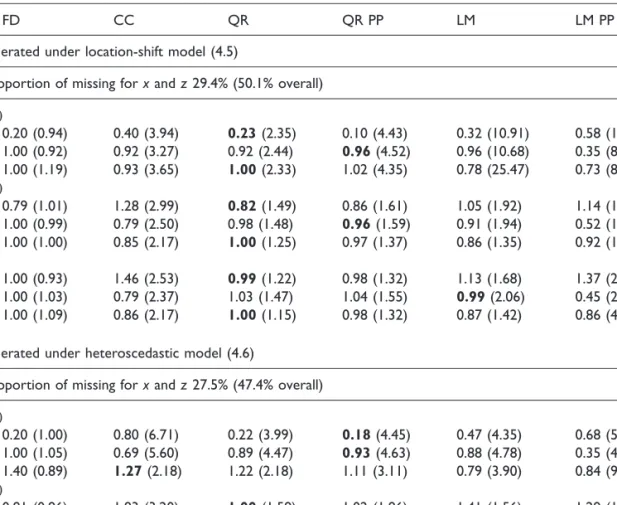
Table 2. Average estimate of the regression coefficients and, in brackets, variance ratio for three analysis models using a complete case analysis (CC) and four different imputation models (QR, QR PP, LM, LM PP). The average model-based estimate using the full datasets (FD) is also reported.
FD CC QR QR PP LM LM PP
Data generated under location-shift model (4.5)
Mean proportion of missing forxandz29.4% (50.1% overall)
Qyjx,zð0:1Þ 0 0.20 (0.94) 0.40 (3.94) 0.23(2.35) 0.10 (4.43) 0.32 (10.91) 0.58 (11.73) 1 1.00 (0.92) 0.92 (3.27) 0.92 (2.44) 0.96(4.52) 0.96 (10.68) 0.35 (8.59) 2 1.00 (1.19) 0.93 (3.65) 1.00(2.33) 1.02 (4.35) 0.78 (25.47) 0.73 (84.84) Qyjx,zð0:5Þ 0 0.79 (1.01) 1.28 (2.99) 0.82(1.49) 0.86 (1.61) 1.05 (1.92) 1.14 (1.58) 1 1.00 (0.99) 0.79 (2.50) 0.98 (1.48) 0.96(1.59) 0.91 (1.94) 0.52 (1.81) 2 1.00 (1.00) 0.85 (2.17) 1.00(1.25) 0.97 (1.37) 0.86 (1.35) 0.92 (1.47) Eðyjx,zÞ 0 1.00 (0.93) 1.46 (2.53) 0.99(1.22) 0.98 (1.32) 1.13 (1.68) 1.37 (2.40) 1 1.00 (1.03) 0.79 (2.37) 1.03 (1.47) 1.04 (1.55) 0.99(2.06) 0.45 (2.64) 2 1.00 (1.09) 0.86 (2.17) 1.00(1.15) 0.98 (1.32) 0.87 (1.42) 0.86 (4.70)
Data generated under heteroscedastic model (4.6)
Mean proportion of missing forxandz27.5% (47.4% overall)
Qyjx,zð0:1Þ 0 0.20 (1.00) 0.80 (6.71) 0.22 (3.99) 0.18(4.45) 0.47 (4.35) 0.68 (5.83) 1 1.00 (1.05) 0.69 (5.60) 0.89 (4.47) 0.93(4.63) 0.88 (4.78) 0.35 (4.31) 2 1.40 (0.89) 1.27(2.18) 1.22 (2.18) 1.11 (3.11) 0.79 (3.90) 0.84 (9.41) Qyjx,zð0:5Þ 0 0.81 (0.96) 1.83 (3.20) 1.00(1.59) 1.02 (1.86) 1.41 (1.56) 1.29 (1.64) 1 0.99 (0.96) 0.58 (2.72) 0.89 (1.68) 0.92(1.84) 0.87 (1.90) 0.47 (1.55) 2 2.57 (1.11) 2.27 (2.13) 2.36(1.28) 2.26 (1.39) 1.94 (0.76) 2.22 (1.58)
from the full dataset (FD), i.e. bFD¼2001 P200
j¼1bbj, FD, for each analysis model. We also report the variance ratio defined as the average of the model-based estimated variances divided by the Monte Carlo variance for the FD. The mean absolute difference between point estimates andFD, divided byFD , was used as an approximation of the absolute relative bias.
For data generated under model (4.5), QR imputation outperformed all other methods. Despite the substantial fraction of missing values in each variable and overall, the absolute percentage bias of QR did not exceed 27% across the three analysis models (median 8%) (results not shown). In most occasions, the LM PP method produced heavily biased estimates, with peaks of almost 200% (median 44%), performing even worse than the CC approach. QR imputation was also very competitive in terms of variability, having the lowest variance ratio among the MI methods.
For data generated using the heteroscedastic model (4.6), QR imputation performed well as compared to the other methods. The average estimate of the regression coefficients from the two QR-based MI methods was comparable. LM and LM PP produced estimates less biased than CC in some cases, though LM PP did not perform well as compared to LM since the log-transformation worsened the relative bias of LM estimates in half of cases. The MI methods did not, however, differ greatly by variance ratio.
A sensitivity analysis with m¼10 imputations was carried out, and the results were almost identical to those described above.
Finally, we compared QR with RQR imputation (results not shown). As expected, estimates were insensitive to this adjustment. There was a tendency of RQR imputation to be slightly less efficient than QR imputation, though no meaningful pattern could be identified.
5
MI analysis of birthweight determinants
5.1
Missing data patterns
In this section, we give a detailed account of missing values in the MCS dataset. We also analyse the distribution of the continuous variables. The subscriptj¼1,. . ., 16 will indicate the variables as numbered in Table 1 (e.g.z1 is birthweight andr1 is its missing data indicator).
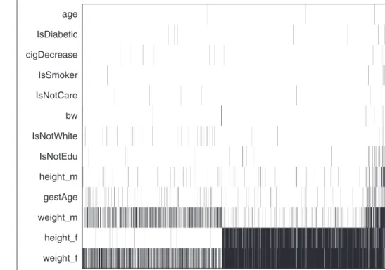
A visual summary of the missing pattern is given in Figure 2 which shows that, overall, the pattern is nonmonotone. The most frequent missing data patterns involved parental body size measures. In particular, paternal weight and height were both missing for 9% of all children (15,070), followed by paternal weight only (5%) and maternal weight only (3%). Each of all the other patterns occurred in less than 1% of the sample.
In the MCS, birthweights were obtained from interviews. Maternal recall of birthweight has been shown to be reliable, although with few exceptions.80We found a significant association between the missing indicators r1 andr2 (2 testp value 50:001), with birthweight more likely to be missing when gestational age was missing, and vice versa. In particular, the odds of gestational age being missing in women with no education and in those of non-white ethnicity were, respectively, 4 (pvalue 50:001) and 3 (pvalue 50:001) as compared to the baseline. There was also a positive association with parity (pvalue 0.03). This is consistent with reported findings80that MCS mothers from ethnic wards, of non-white ethnic group, unemployed and with non-zero parity were more likely than others to provide an estimate of their child’s birthweight that differed from the birth registration’s recorded value by 100g or more. Similarly to what suggested by Tate et al.,80cultural differences and language barriers could also partly explain missingness for these variables. It is
reasonable to assume that conditionally on ethnicity, parity and the stratification variable, the missing data mechanism for birthweight and gestational age is ignorable.
Missing paternal weight and height accounted for 76% of the total number of incomplete cases (3066). There was a significant association between the missing indicators r5 and r6 (p value
50:001). However, the missing data pattern showed some degree of monotonicity (Figure 2). It could be inferred that the respondents (i.e. the mothers) were able to recall their partners’ height more easily that their weight, as the latter is subject to greater variation. Failing to give a measure of their partners’ height implied having a poor ability to provide information on weight as well. Again, we assume a MAR mechanism for paternal weight and height as well as for the rest of the variables with missing items.
5.2
The imputation models
We now consider estimating the analysis model (3.4) after MI using the FCS algorithm described in Section 4 and we discuss some related modelling issues.
First, we establish which design variables to include in the imputation model, starting with cluster effects. We calculated complete case intraclass correlation coefficients (ICC) for all variables in Table 1, except reduction in number of cigarettes smoked (variable 9). We found that the ICC varied between 0.01 and 0.12 for variables 1–8 and between 0 and 0.22 for variables 10–13, 15, and 16. As expected, the highest ICC was seen in mother’s ethnicity (0.55) as this variable falls in one of the stratification domains. However, its fraction of missing values accounts for only 0.3% of the sample size. On this basis, we decided not to include clustering in the
weight_f height_f weight_m gestAge height_m IsNotEdu IsNotWhite bw IsNotCare IsSmoker cigDecrease IsDiabetic age
Figure 2. Missing data pattern in the MCS sample. Observations (x-axis) and variables (y-axis) are ordered by number of missing values. Black denotes missing.
imputation procedure as if would have been uninformative and the large number of clusters (400) would have increased the computation time.
The MCS design stratification variable was found to be strongly associated with most of the variables. Sampling strata were therefore included in the conditional specification as categorical, so were sampling weights as continuous. The associated data matrixZwhich was fed intomice had dimensions 15,0708. For comparison purposes, a larger imputation model was also considered including stratum-specific effects (except for gestational age, and prenatal care and diabetes status indicators which were not found to be significantly associated with the stratification variable). As a result, the number of columns ofZincreased from 18 to 121.
Next, we make some considerations about the continuous variables (we leave out age at delivery since the number of missing values in this variable is very small). The histogram of birthweight by gestational age and the histogram of gestational age were provided in Figure 1. Table 3 shows skewness, kurtosis, estimated (marginal) BCT parameter and p value of the Shapiro–Wilk test for normality after BCT. In all cases, skewness and excess kurtosis are apparent while the BCT fails to achieve normality even when these are relatively moderate, as in the case of paternal weight. Normal Q-Q plots (not shown) confirmed this result. This suggests that using mean regression as imputation model would be inappropriate.
Two pairs of variables are of particular interest in relation to MI: birthweight and gestational age, and paternal weight and height. The former pair includes the response variable and its strongest predictor (Spearman’s rank correlation 0.42), while the latter includes two strongly correlated (0.47) variables with the highest proportion of missing values among all other variables. These are plotted in Figure 3 using logit scaling on the y-axis. There is an indication that a linear relationship is reasonable. Note also the outlying observations in both plots (this point will be discussed further in Section 5.4).
We tested location shift and location-scale shift hypotheses by using Khmaladze tests76 for the linear models logitðbwÞ gestAge (sample sizen¼14,907) and logitðweightfÞ heightf(n¼12,731) on the rangep2½0:05, 0:95 . None of the tests rejected the null hypothesis at the 5% level except for the location shift hypothesis in the birthweight model. We repeated the tests for bw gestAge and weightf heightf. The location-scale shift hypothesis for birthweight and the location shift hypothesis for paternal weight were rejected at the 1% and 5% level, respectively. In summary, these results suggest the following: on the untransformed scale, the relationship between birthweight and gestational age is more complex than a location-scale shift model; in contrast, the relationship between paternal weight and height can be defined by a heteroscedastic model. On the logit scale, the former relationship is approximately heteroscedastic whereas the latter relationship is approximately constant over quantiles. In other words, the logit transformation has simplified the model specification.
Finally, we assigned an imputation model to each variable with missing data (Table 1). More precisely, continuous variables (1–7, 9) were imputed using the QR-based approach described in
Table 3. Analysis of shape for selected MCS continuous variables.
bw gestAge weightm heightm weightf heightf
Skewness 0.52 2.26 1.20 0.11 0.58 0.23
Kurtosis 4.95 12.30 5.40 5.02 3.83 4.36
1.60 10.40 0.80 1.60 0.00 2.40
Section 4.2. In particular, we set!equal to 0.001 in step (i). Since these variables are constrained to vary within boundaries, pre-processing was carried out by applying a logit transform with internal bounds which, as seen above, gives an additional benefit for modelling. Binary variables (10, 11, 14–16) were assigned logistic regressions.
We setm¼5 imputed datasets and a maximum of five iterations for each imputation. These are the default values in theRfunctionmi.48The QR model (3.4) was then fitted to each imputed dataset using the methods illustrated in Section 4.1. As in the complete case analysis (Section 3.2), a bootstrap sample sizenB¼100 was used to estimate the variance of the regression quantiles.
5.3
Results
First and foremost, the results of the analysis did not differ sensibly when using the ‘reduced’ (i.e. with strata effects only) or the ‘full’ (i.e. with stratum-specific effects) imputation models. Table 4 shows point estimates and standard errors for selected quantiles (results for all quantiles are available upon request) using the reduced model. In the following, we elaborate on parental and smoking effects which offer elements of novelty but we gloss over the other effects for the sake of brevity.
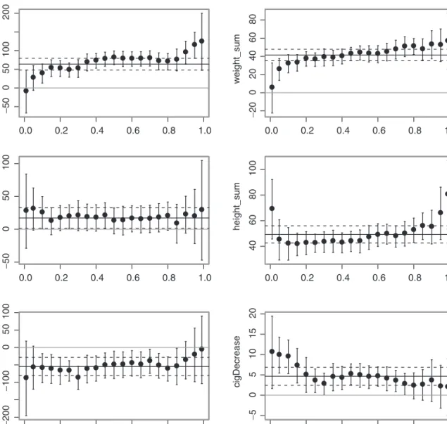
The complete sets of estimated regression quantiles for differential and mean parental weight and height are plotted in Figure 4. The coefficients of differential weight were positive and significant (p
value 50:05) for quantiles p0:1, with larger magnitude at higher quantiles. For p¼0:01 and
p¼0:05, 2ðpÞ was not significantly different from zero at the 5% level. Similarly, the quantile effects of parental mean weight were positive for allpand the magnitude of these effects was larger at higher birthweight quantiles.
The quantile effects of differential parental height had large confidence intervals. However, the least squares estimate was marginally significant (p value 50:05). Mean parental height had a
60 65 70 75 80 −10 −5 5 01 0 gestAge Logit (bw) 120 140 160 180 200 − 4 − 22 04 height_f Logit (weight_f)
Figure 3. Left: birthweight versus gestational age. Right: paternal weight versus height. Theyaxis is on the logit scale.
positive effect on all birthweight quantiles and such effect was approximately uniform, except at the extremes where the coefficients were larger.
These results are consistent with those reported by Griffiths et al.63In their study based on MCS data, a regression model for mean birthweight was fitted after incomplete parental data were discarded under MCAR assumptions. In contrast, we allowed for variables such as maternal education and ethnicity to account for a MAR data mechanism. Our analysis shows that the parental effects are not constant across the birthweight distribution. This provides important insights for the understanding of the parental conflict theory81 according to which the father’s aim is to maximize the growth of his offspring, while mothers maximize their chance of survival by constraining foetal growth. As reported by Griffiths et al., the influence of the mother wins over the father’s contribution to mean birthweight. However, it seems that this influence is somehow relaxed when the survival of the child is at high risk (low birthweight quantiles) and it is strongest at the opposite end of the range (high birthweight quantiles) when her own survival is at higher risk. In other words, there may be an effect gradient in the anthropometric parental factors regulating birthweight that runs from top to bottom of the birthweight spectrum. To the best of our knowledge, these results have not been reported before and deserve further investigation.
Smoking is known to reduce birthweights82 and this effect is approximately uniform across birthweight quantiles, as confirmed by our results (Figure 4). Although on average a decrease in smoking had little effect on birthweight (approximately 5 g per cigarette per day), at lower quantiles the coefficient was twice as much (approximately 10 g per cigarette per day). Such effect was attenuated at higher quantiles. Despite the different design and purpose of our analysis as
Table 4. Point estimates of selected regression quantiles and, in brackets, standard errors for the MCS birthweight analysis.
Complete case analysis Multiple imputation analysis
Quantile Quantile 0.05 0.5 0.95 0.05 0.5 0.95 Intercept 2340(28) 3006(15) 3778(38) 2354(24) 3010(12) 3784(32) gestAge 174(6) 168(4) 128(9) 170(5) 169(3) 129(8) weighthd 20 (18) 82(11) 119(16) 19 (17) 80(9) 114(17) weightsum 26(7) 45(4) 53(10) 28(7) 43(4) 53(9) heighthd 37(16) 12 (11) 22 (22) 30(16) 11 (10) 20 (21) heightsum 44(8) 46(4) 68(11) 45(8) 45(4) 67(10) age 2 (2) 0 (1) 1 (3) 2 (2) 0 (1) 1 (2) parity 58(11) 69(7) 88(18) 50(10) 62(6) 81(15) cigDecrease 10(2) 5(2) 1 (3) 10(2) 5(2) 2 (3) IsSmoker 56 (31) 58(22) 23 (41) 51 (31) 51(20) 20 (39) IsNotEdu 95(34) 22 (21) 30 (39) 84(29) 15 (19) 39 (32) IsGirl 116(21) 139(10) 108(26) 112(20) 143(9) 105(24) IsNotMarried 46 (29) 10 (16) 23 (28) 37 (22) 12 (14) 16 (28) IsNotWhite 149(37) 137(24) 32 (33) 203(35) 162(19) 42 (31) IsNotCare 33 (63) 56 (31) 147 (161) 39 (51) 30 (27) 61 (133) IsDiabetic 43 (77) 80(31) 182 (142) 83 (115) 88(29) 164 (149)
compared to England et al.,82 our results point out the different impact on birthweight that a reduction in smoking has at different birthweight quantiles.
Similar conclusions were reached when using the results from the complete case analysis (Table 4). In general, the latter provided estimated coefficients that were consistent with those obtained after MI, except for the effect associated with ethnicity. The magnitude of this coefficient was, on average, about 26% larger after imputation. This is not surprising given that ethnicity is a strong predictor of MCS unit nonresponse51and missing birthweight. It also falls in one of the stratification domains. In contrast, the standard errors of the coefficients after imputation tended to be lower than those obtained in the complete case analysis by about 10%, on average. This
● ● ●● ● ● ● ● ● ●● ● ● ● ● ● ● ●● ● ● 0.0 0.2 0.4 0.6 0.8 1.0 − 50 0 50 100 200 weight_hd ● ●● ●● ● ● ● ● ● ● ● ● ● ●● ● ● ● ● ● 0.0 0.2 0.4 0.6 0.8 1.0 − 20 0 20 40 60 80 weight_sum ● ● ● ● ● ●● ● ● ● ● ● ● ● ● ● ●●● ● ● 0.0 0.2 0.4 0.6 0.8 1.0 − 50 0 50 100 height_hd ● ● ● ● ● ● ● ● ● ● ●● ● ● ● ●● ● ● ● ● 0.0 0.2 0.4 0.6 0.8 1.0 40 60 80 100 height_sum ●● ● ● ● ●●● ● ● ● ●● ● ● ● ● ● ●● ● 0.0 0.2 0.4 0.6 0.8 1.0 − 200 − 100 0 50 100 IsSmoker ● ● ● ● ● ● ●● ● ● ● ● ● ● ●● ● ● ● ● ● 0.0 0.2 0.4 0.6 0.8 1.0 − 50 5 1 0 1 5 2 0 cigDecrease
Figure 4. Estimated regression quantiles with 95% confidence intervals (error bars) for parental weight and height and smoking effects in the MCS birthweight analysis. Horizontal black lines denote mean estimates (solid) and their 95% confidence intervals (dashed).
can be explained by a lower within-imputation variance and by a relatively small between-imputation variance, the latter accounting on average for about 5% of the total between-imputation variance.
Sensitivity analyses were carried out, including: an analysis under MCAR and SRS assumptions (i.e. ignoring missingness and sampling design). QR standard errors were calculated using the asymptotic variance estimator forniderrors; an analysis where only sampling weights but not the strata were included in the imputation model; an analysis where strata and unadjusted weights were used. In summary, the design effect for mean and median birthweight was, respectively, 1.8 and 1.9, which indicates that design-based estimates are around 90% less efficient than an SRS for the selected outcome and this justifies the use of survey variables in the analysis model. Not including strata in the imputation model had little effect on the results, as did the use of unadjusted weights. Obviously, this has implications for the analysis of birthweight only as other MCS variables might respond differently to such modelling adjustments. Design effects for other MCS variables that are highly correlated with the sampling domain (e.g. ethnicity, income) can be as high as 20.49
In total, the imputation (reduced model) and analysis steps took about 43 and 24minutes, respectively, on a 64-bit operating system machine with 16 Gb of RAM and quad-core processor at 2.93 GHz. In both steps, we used a Frisch–Newton algorithm as most appropriate given the size of the problem. The Barrodale and Roberts algorithm83 took about twice as long. Reductions of computation time could ideally be obtained by decreasing the number of breakpoints ui in the imputation step and by employing parallel computing in the analysis step. Changing the variables visiting sequence48from that in Table 1 to a sequence in increasing order of missing data did not provide an appreciable computational advantage.
5.4
Diagnostics
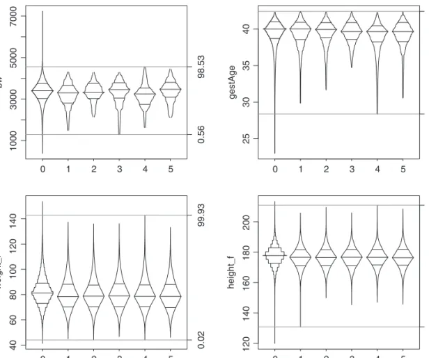
MI methods are typically accompanied by diagnostic measures to assess the imputed values and the impact of the missing data on the parameters being estimated. In Figure 5, box-centile plots of observed and imputed values for four selected variables are reported. The distribution of each imputed sample follows the observed distribution reasonably well. The coverage of the observed range by the imputed values is nearly 100% and, as a consequence of the logit transformation, in no case the range is exceeded. A similar imputation without pre-processing (results not shown) produced values for parental weight and height outside the observed range.
Although the distributions of birthweight and gestational age stretch to very low and high points, more extreme values were implicitly excluded by trimming the distribution ofzwhen defining upper and lower limits foru, that isu Unifð0:001, 0:999Þ. In general, conditional quantiles are robust to outliers in the outcome but may be sensitive to outliers in the design matrix. As mentioned in Section 2, several outliers in parental weight were replaced by missing values. Outliers were defined as observations exceeding the quantiles 0.0005 and 0.9995 of these variables. In total, we detected 16 and 14 values (as low as 11kg and as high as 288kg) for, respectively, maternal and paternal weight. Although this method is naı¨ve and a more sensible outlier detection approach could have been based on the bivariate distribution of weight and height, it is of little practical importance in our analysis since our aim is to assess the value of the outliers as compared to their imputed values. Figure 6 shows the bivariate plot of height and weight for both parents. In addition to the formal testing conducted earlier, the strong heteroscedasticity that characterizes the relationship between these two variables can now be seen. This distributional feature is taken into account by the QR-based imputation model as shown by the range of imputed values at different heights. For example, very low paternal weights defined as outliers had imputed values that were consistent with the
given height, and the spread of such imputations was consistent with the spread of the observed distribution of weight at that given height. A mean regression would not be able to preserve such distributional relationships between variables.
For each regression quantile, the rate of missing information (RMI) can be calculated as ¼rþ2r=þðdf1þ3Þ, where r¼ 1þm
1
ð Þ
^
ðpÞ , df is the number of degrees of freedom and b is the
between-imputation variance. Overall, the maximum RMI was approximately 20% and this was observed for weighthd. The latter variable was obviously affected by a substantial increase in variance due to a high proportion of missing values of paternal weight. The RMI for gestational age did not exceed 8% in all quantiles but it was higher for the first regression centile (7%) as compared to the 99th (2%).
Finally, we checked the mean and variance of the imputed values at each iteration for all but the discrete variables and no systematic pattern was observed.
1000 3000 5000 7000 bw 0 1 2 3 4 5 0.56 98.53 25 30 35 40 gestAge 0 1 2 3 4 5 0.32 100 40 60 80 100 120 140 weight_f 0 1 2 3 4 5 0.02 99.93 120 140 160 180 200 height_f 0 1 2 3 4 5 0.02 99.99
Figure 5. Box-centile plots of observed (0) and imputed (1–5) values for birthweight, gestational age, paternal weight and height. Grey lines define the centile range of coverage of the observed distribution by the minimum and maximum of all imputed values.
6
Discussion
Complex survey estimation and MI are two important statistical areas in the analysis of large population-based epidemiological and socioeconomic studies. In this paper, we considered the application of quantile modelling to the analysis of birthweight determinants in a cohort of UK children, providing an extensive and detailed investigation of methods that can be easily implemented using available software and little additional programming effort. The problem of missing data was addressed by developing an MI approach under MAR assumptions, based on an FCS algorithm in which imputation of continuous variables takes into account the distributional features of the observed data. We discussed model selection issues associated with MI in general and QR-based imputation in particular and explored some practical aspects in the MCS analysis.
We proposed some strategies on how to use transformations for handling outliers and bounded variables, and, in the MCS birthweight study, we showed that transformations may also be beneficial to the specification of the form of quantile functions. However, transformations that are typically considered as a remedy for data that do not conform to some well-known distribution are often unsatisfactory, may require estimating additional parameters, and pose delicate problems for interpreting the results. Features such as skewness or kurtosis, which is traditionally associated with peakedness and tail weight of a distribution, are not to be seen as a nuisance but rather as informative on the unknown data-generating process. Moreover, their conditional relationship with the covariates under study is often too complex to benormalized by a simple marginal transformation. In contrast, quantiles are able to discriminate among distributional shapes in a natural way, as also demonstrated by an increasing number of proposals of quantile-based measures of asymmetry and kurtosis.84–86 QR offers a flexible and powerful means to preserve the information in the data. In addition, it handles desired data transformations in a simple yet mathematically rigorous fashion.
But the flexibility associated with QR may come at a cost: the difficulty in choosing among a number of models for different quantiles. As stressed by Van Buuren38 and Schafer,75 avoiding
20 40 60 80 100 weight_m 120 140 160 0 50 100 150 200 weight_f 250 300 100 120 140 160 height_m 180 200 120 140 160 height_f 180 200
Figure 6. Plot of observed weight versus height (grey dots) for MCS mothers and fathers. Crosses denote weight outliers while black dots the corresponding imputations.
specifying a joint distribution for the data and the missing data mechanism does not clearly remove other model selection issues. Moreover, accounting for the sampling design variables in the MI procedure can be laborious from a computational and a modelling standpoint. In addition, analytical demonstration that the imputation is ‘proper’65 may be difficult except in trivial cases.64, p. 145
It is worth stressing that analysis and imputation models need not be the same. It is, of course, a logical consequence that a location-shift hypothesis for the imputation model is incompatible with the motivation that has led, in the first place, to a conditional quantile approach for the model of interest. Separating imputation and analysis models can be advantageous.75 In non-normal conditions, QR-based imputation is an excellent alternative to mean imputation when the target of the analysis is the conditional mean,39even when the data undergo some form of pre-processing as shown in our simulation study. It needs to be investigated whether other inferential targets (e.g. scale and shape indices) can benefit from this approach.
Funding
The Centre for Paediatric Epidemiology and Biostatistics benefits from funding support from the Medical Research Council in its capacity as the MRC Centre of Epidemiology for Child Health (G0400546). The UCL Institute of Child Health receives a proportion of funding from the Department of Health’s NIHR Biomedical Research Centres funding scheme.
Acknowledgements
We thank two anonymous reviewers, whose constructive comments led to an improved manuscript; Jianqiang Wang and Jean Opsomer who kindly provided theRcode to replicate their simulation study; and Matteo Bottai for providing a copy of the paper entitled ‘Multiple imputation based on conditional quantile estimation’.
References
1. Smith K and Joshi H. The Millennium Cohort Study.
Popul Trends2002;107: 30–34.
2. Koenker R and Bassett G. Regression quantiles.
Econometrica1978;46: 33–50.
3. Yu KM, Lu ZD and Stander J. Quantile regression: applications and current research areas.J R Stat Soc Ser D 2003;52: 331–350.
4. Machado JAF and Santos Silva JMC. Quantiles for counts.J Am Stat Assoc2005;100: 1226–1237. 5. Portnoy S. Censored regression quantiles.J Am Stat Assoc
2003;98: 1001–1012.
6. Bottai M and Zhang J. Laplace regression with censored data.Biom J2010;52: 487–503.
7. Bottai M, Cai B and McKeown RE. Logistic quantile regression for bounded outcomes.Stat Med2009;9: 309–317.
8. Yu KM and Jones MC. Local linear quantile regression.
J Am Stat Assoc1998;93: 228–237.
9. Koenker R, Ng P and Portnoy S. Quantile smoothing splines.Biometrika1994;81: 673–680.
10. Thompson P, Cai YZ, Moyeed R, et al. Bayesian nonparametric quantile regression using splines.Comput
Stat Data Anal2010;54: 1138–1150.
11. Heagerty PJ and Pepe MS. Semiparametric estimation of regression quantiles with application to standardizing weight for height and age in US children.J R Stat Soc Ser C1999;48: 533–551.
12. Lee D and Neocleous T. Bayesian quantile regression for count data with application to environmental
epidemiology.J R Stat Soc Ser C2010;59: 905–920. 13. Koenker R and Geling O. Reappraising medfly longevity.
J Am Stat Assoc2001;96: 458–468.
14. Koenker R.Quantile regression. New York: Cambridge University Press, 2005.
15. Abrevaya J. The effects of demographics and maternal behavior on the distribution of birth outcomes.Empir Econ2001;26: 247–257.
16. Abrevaya J and Dahl CM. The effects of birth inputs on birthweight: evidence from quantile estimation on panel data.J Bus Econ Stat2008;26: 379–397.
17. Burgette LF and Reiter JP. Modeling adverse birth outcomes via confirmatory factor quantile regression.
Biometrics2012;68: 92–100.
18. Burgette LF, Reiter JP and Miranda ML. Exploratory quantile regression with many covariates: an application to adverse birth outcomes.Epidemiology2011;22: 859–866. 19. Mudd LM, Pivarnik J, Holzman CB, et al. Leisure-time
physical activity in pregnancy and the birth weight distribution: where is the effect?J Phys Act Health2012;9: 1168–1177.
20. Bo¨rnhorst C, Hense S, Ahrens W, et al. From sleep duration to childhood obesity – what are the pathways?