Socioeconomic Institute
Sozialökonomisches Institut
Working Paper No. 0913
Copula-based bivariate binary response models
Rainer Winkelmann
Socioeconomic Institute University of Zurich Working Paper No. 0913
Copula-based bivariate binary response models
August 2009
Author's address: Rainer Winkelmann
E-mail: [email protected]
Publisher Sozialökonomisches Institut
Bibliothek (Working Paper) Rämistrasse 71 CH-8006 Zürich Phone: +41-44-634 21 37 Fax: +41-44-634 49 82 URL: www.soi.uzh.ch E-mail: [email protected]
Copula-based bivariate binary response models
Rainer Winkelmann∗University of Zurich August 2009
Abstract
The bivariate probit model is frequently used for estimating the effect of an endogenous binary regressor on a binary outcome variable. This paper discusses simple modifications that maintain the probit assumption for the marginal distributions while introducing non-normal dependence among the two variables using copulas. Simulation results and evidence from two applications, one on the effect of insurance status on ambulatory expenditure and one on the effect of completing high school on subsequent unemployment, show that these modified bivariate probit models work well in practice, and that they provide a viable and simple alternative to the standard bivariate probit approach.
JEL Classification: C23
Keywords: Bivariate probit, binary endogenous regressor, Frank copula, Clayton copula.
∗
Address for correspondence: University of Zurich, Socioeconomic Institute, Zurichbergstr. 14, CH-8032 Zurich, Switzer-land, phone: +41 (0)44 634 22 92, fax: +41 (0)44 634 49 96, email: [email protected]; I thank Murray Smith, Kevin Staub as well as seminar participants at the University of Maryland, Georgetown University and Johns Hopkins University for helpful discussions and suggestions.
1
Introduction
The bivariate probit model provides a convenient setting for estimating the effect of an endogenous binary regressor on a binary outcome variable. The generic recursive version of the model can be expressed as
y1 =1(x0β+αy2+ε1 >0) (1)
y2 =1(z0γ+ε2>0) (2)
where 1(·) is the indicator function and x and z are vectors of covariates. The main interest is in the structural parameter α, and it is assumed that ε1 and ε2 have a bivariate standard normal distribution
(independently of xand z) with correlationρ:
F(ε1, ε2) = Φ2(ε1, ε2, ρ) (3)
It follows that the joint conditional probability functionf(y1, y2|x, z) is given by
f(y1, y2|x, z) = Φ2[s1(x0β+αy2), s2(z0γ), s1s2ρ] (4)
wheres1 = 2y1−1 and s2 = 2y2−1. For α = 0, (4) reduces to a “seemingly unrelated” model. Closely related is the sample selection model where
y1 =1(x0β+ε1 >0)
is observed ifz0γ+ε2 >0, and unobserved else.
The bivariate probit model has been used in numerous economic applications, among them the effect of attending catholic high school on graduation (Evans and Schwab, 1995, Vella, 1999), the effect of early childbearing on high school completion (Ribar, 1994), the effect of insurance status on mortality (Bhat-tacharya et al., 2006), the effect of hospital type on delivery by Cesarean section (Fabbri and Monfardini, 2008), and the effect of receiving any first-year financial aid on completing a Ph.D. program within five years (Stock et al., 2009), to name but a few.
A key property of the bivariate probit model is that the joint model simplifies to two univariate probit equations under independence (ρ= 0), sinceF(ε1, ε2) has standard normal marginals following from (3). It
is a common view that the bivariate normal distribution is the only (simple) bivariate family of distributions with this property (e.g., Bhattarcharya et al., 2006). The bivariate probit model is, by the same token, seen as the logical generalization of the univariate probit model.
One objective of the paper is to correct this misapprehension. While a given joint distribution defines exactly one set of marginal distributions, the opposite does not hold. In fact, there are infinitely many other joint distribution functionsF(ε1, ε2) with probit marginals.
The second contribution is a novel framework for specification and estimation of alternative bivariate binary response models in a relatively simple parametric setting. This framework integrates the copula approach into the bivariate binary response model defined by (1) and (2).
Any joint distribution function has a copula representation in which the specification of dependence and marginals is explicitly separated, or “uncoupled”. Copulas can be used to build alternative joint distributions that preserve the probit assumption for the marginals but do not impose joint normality. In particular, one can recur to a set of well known parametric families of copula functions that differ in their dependence properties but preserve the simplicity of the bivariate probit.
These models are potentially useful in situations where one has confidence in the specification of the probit marginals but worries about misspecification of the dependence structure of the bivariate probit model. For example, the conditional expectation function E(ε1|ε2) may be non-linear rather than linear,
as implied by the bivariate probit.
In this paper, three parametric copula functions are investigated in the context of the bivariate binary response model: the Normal copula, Frank’s copula and Clayton’s copula. Having derived the three copula representations for the bivariate model, a series of Monte Carlo simulations show that it is possible to empirically discriminate between the different copulas. Furthermore, using a wrong copula can lead to substantial bias in the estimation of structural parameters.
Finally, the new approach is illustrated in real data examples, first an application to the endogeneity of insurance choice in a model for ambulatory health expenditures, following Deb, Munkin, and Trivedi (2006), and second an application relating to the joint determination of high school completion and post-school unemployment incidence, based on Li (2006).
2
The Model
2.1 Copula Functions
Copulas offer a convenient representation of arbitrary joint distribution functions, with the key property being that the specification of the marginal distributions and the dependence structure is separated. The earliest copula use in econometrics was Lee (1983) who suggested, in the context of a sample selection model, to use a bivariate normal copula for generating dependence between two continuous random variables, one with normal marginal (the continuous outcome variable) and one with logistic distribution (the error in the latent selection equation). The first econometric applications to discrete outcomes were provided by van Ophem (1999, 2000) who used a bivariate normal copula to generate joint distributions for two random variables with Poisson/Poisson and Poisson/normal marginals, respectively.
The systematic consideration of non-normal copulas started with Smith (2003) who specified eight dif-ferent copulas for normal/normal and normal/gamma marginals. Further contributions in this area include Smith (2005) who used five different copulas in a switching regression model for continuous outcomes, and Zimmer and Trivedi (2006) who used the Frank copula for negative binomial/normal marginals. An intro-duction to the copula method for empirical economists is provided by Trivedi and Zimmer (2007), see also Nelson (2006).
Formally, a copula is a multivariate joint distribution function defined on the n-dimensional unit cube [0,1] such that every marginal distribution is uniform on the interval [0,1]. For example, the normal, or Gaussian, copula, forn= 2, is
P(U ≤u, V ≤v) =C(u, v) = Φ2(Φ−1(u),Φ−1(v);θ) (5)
where Φ and Φ2 are the uni- and bivariate cdfs of the standard normal distribution, andθis the coefficient
of correlation. Two examples for copulas with closed form expressions are Clayton’s copula
C(u, v) = (u−θ+v−θ−1)−1/θ (6)
and the Frank copula
C(u, v) =−θ−1log ( 1 +(e −θu−1)(e−θv−1) (e−θ−1) ) (7)
The marginal distributions are given by P(U ≤ u, V ≤ 1) = C(u,1) and P(U ≤ 1, V ≤ v) = C(1, v), respectively. It is easy to verify that all three copulas have the property that their marginal distributions are uniform, asC(u,1) =u and C(1, v) =v.
The significance of copulas lies in the fact that by way of transformation, they can be used to generate joint distribution functions for random variables with arbitrary, non-uniform marginals. Let u = Fx(x)
andv =Fy(y). ThenG(x, y) =C(Fx(x), Fy(y)) is a joint distribution function for xand y with marginal
distribution functionsFx(x) and Fy(y). Even more importantly, a theorem due to Sklar (1959) says that
any joint distribution function can be expressed as a copula applied to the marginal distributions, and that this representation is unique for continuous random variablesx and y.
The practical significance of copula functions in empirical modeling derives from the fact that they can be used to build new multivariate models for given univariate marginal component cdf’s. If the bivariate cdfF(x, y) is unknown, but the univariate marginal cdf’s are of known form, then one can choose a copula function and thereby generate a representation of the unknown joint distribution function. The key is that this copula function introduces dependence, captured by additional parameter(s), between the two random variables (unless the independence copula C(u, v) = uv is chosen). The degree and type of dependence depends on the choice of copula.
I consider four copula functions in this paper, the normal copula, Frank’s copula, Clayton’s copula, and the independence copulaC(u, v) =uv. The marginals are standard normal in each case, corresponding to standard probit models for the two binary dependent variables under independence. The normal copula model is then equivalent to the bivariate normal distribution, as
F(x, y) = Φ2[Φ−1(Φ(x)),Φ−1(Φ(y))] = Φ2(x, z)
To describe the differences in the dependence structure implied by these copulas, correlation is not a good summary statistic. First, it detects only linear dependence, whereas dependence in copulas is non-linear in general. Second, and relatedly, it is not invariant to transformation of the marginals. As a consequence, other measures have to be used, and a common one is Kendall’sτ, a measure of the degree of concordance. Imagine drawing to random pairs (U1, V1) and (U2, V2) from the joint distribution ofU and V. Then τ is
defined as
τ =P[(U1−U2)(V1−V2)>0]−P[(U1−U2)(V1−V2)<0]
τ can vary between -1 and 1. It is zero if U and V are independent. Not all copulas cover the full spectrum of possibleτ’s. If they do so, they are called comprehensive. The normal and Frank copulas are comprehensive, the Clayton copula (6) is not, the reason being that it only captures positive dependence. It is “half comprehensive”, however, since τ can take any value between 0 and 1. Of course, one can always reflect a Clayton copula, modeling the relationship betweenU and −V instead, in which case the dependence is strictly negative, withτ’s between -1 and 0.
Additional insight into the nature of dependence implied by these copula models can be obtained from contour plots of the joint density function or, alternatively, the conditional expectation functions (CEFs). Both are not invariant to the choice of marginal distribution. In this paper, the interest is in standard normal marginals that correspond to the probit assumption. The CEF of the bivariate normal distribution is linear, with E(Y|X =x) =ρx. For the Clayton and Frank copula, simple expressions for the conditional expectations are not available, but it is straightforward to obtain them by way of simulation. Figures 1 and 2 show a sample of 500 draws from the Frank and Clayton copulas, with standard normal marginals, forθ= 3.3 andθ= 1, respectively. Also shown are the CEFs (obtained from a nonparametric regression) as well as the linear regression line.
The Frank copula is symmetric. Its CEF is near linear in the center but flattens out in the tails. This is an interesting feature that may be of interest in applications to sample selection models where the linearity of the CEF of the bivariate normal distribution lacks plausibility when selection probabilities are very small. The Clayton copula looks quite different. It is not symmetric, and the CEF shows much stronger dependence in the left tail of the distribution than in the right. Again, this is a distinctive feature that may be a-priori desirable in some applications. Finally note that the tail behavior of the CEF is not directly related to the concept of “tail dependence” that is used in finance. (Upper) tail dependence is defined as the left limit, forv → 1, of the expression P(U > u|V > v). For the normal copula, these two events are independent in the limit, although the CEF is linear. Other copulas (among them thetcopula) allow for
tail dependence.
2.2 Likelihood function for the bivariate binary response model
The bivariate binary response model defined by (1) and (2) has a generic probability function defined by four terms:
P(y1 = 0, y2 = 0|x, z) =P(ε1 ≤ −x0β, ε2 ≤ −z0γ)
P(y1 = 1, y2 = 0|x, z) =P(ε1 >−x0β, ε2 ≤ −z0γ)
P(y1 = 0, y2 = 1|x, z) =P(ε1 ≤ −x0β−α, ε2>−z0γ)
P(y1 = 1, y2 = 1|x, z) =P(ε1 >−x0β−α, ε2>−z0γ)
Under a copula representation with probit marginals, these can be written as
P(y1 = 0, y2 = 0) =C[Φ(−x0β),Φ(−z0γ)] (8)
P(y1 = 1, y2 = 0) =C[1,Φ(−z0γ)]−C[Φ(−x0β),Φ(−z0γ)] (9)
P(y1 = 0, y2 = 1) =C[Φ(−x0β−α),1]−C[Φ(−x0β),Φ(−z0γ)] (10)
P(y1 = 1, y2 = 1) = 1−C[Φ(−x0β−α),1]−C[1,Φ(−z0γ)] +C[Φ(−x0β−α),Φ(−z0γ)] (11)
The joint probabilities depend on the selected copula as well as on four parameters, ξ = (β, γ, α, θ), whereθ is the dependence parameter of the copula function. If the true copula is assumed to belong to a parametric familyC ={Cξ, ξ∈Ξ}, a consistent and asymptotically normally distributed estimator of the
parameterξ can be obtained through maximum likelihood method.
Assuming an independent sample ofnobservations (yi1, yi2, xi, zi), the likelihood functionL(ξ;y1, y2, x, z)
is proportional to
n Y
i=1
×P(yi1= 0, yi2= 1)(1−yi1)yi2×P(yi1 = 0, yi2 = 0)(1−yi1)(1−yi2)
Numerical optimization methods can be used to maximize this function. These can employ analytical first derivatives that have a relatively tractable form. For example,
∂P(y1 = 0, y2= 0|ξ)
∂β =−cu[Φ(−x
0β),Φ(−z0γ)]φ(−x0β)x
where cu = ∂C(u, v)/∂u. A formal requirement for identification is that there is at least one exogenous
regressor with a non-zero coefficient, i.e., β 6= 0 or γ 6= 0 (Wilde, 2000). The maximum likelihood estimator has the usual asymptotic properties, as long as the model is correctly specified. Perhaps it is more pertinent to think of these estimators as providing best approximations to an unknown true model, in a quasi-likelihood sense (White, 1982), and then a robust covariance estimator should be used.
3
A Simulation Study
To explore the performance of the maximum likelihood estimator under the various copula assumptions, I report results for a small simulation experiment designed to evaluate the bias and accuracy of the estimators as well as model selection.
The data generating process (DGP) is a simple recursive model for two binary dependent variables with probit margins:
y1 =1(β0+β1x+αy2+ε1>0)
y2 =1(γ0+γ1z+ε2 >0)
where (β0, β1, γ0, γ1, α) = (0.5,−0.5,0,1,0.5). In all cases x and z are iid Gaussian with mean zero and standard deviation 1.
The stochastic errors ε1 and ε2 are generated from three alternative copula functions:
• Normal copula withρ= 0.5
• Clayton copula withθ= 1
The dependence parameters have been chosen to yield the same value for τ in all three cases, namely 0.33. The marginals are standard normal, meaning that a probit link applies to both y1 and y2 at the
marginal level under independence. Given the parameter values and the distribution ofxand z, the mean of y1 is approximately 73%, while the mean of y2 is approximately 50%. The simulations are conducted for three sample sizesn= 500,1000,5000, and run for r= 5000 replications each.
The results are shown in Table 1 (Normal DGP), Table 2 (Frank DGP) and Table 3 (Clayton DGP). When looking at the results, there are two key questions of interest. First, what are the biases that result from estimating the wrong model?; and second, do tests and model selection reveal the right model? In Table 1, for example, the parameter of the exogenous regressor β1 (the true value is -0.5) is estimated
well regardless of model and sample size. (Similarly, the means of the estimated parameters forγ0 and γ1
do not show any systematic deviations from their true values and hence are not reported in the tables.) However, the parameter of the endogenous regressor α is subject to bias in the misspecified models. The bias is very large for the independence model, where it amounts to over 100 % but there is also substantial bias for the Clayton copula. For n= 500, for instance, the Clayton mean is 0.549, compared to the true value of 0.5. The bias does not vanish as the sample size increases.
The average likelihood ratio test statistic for the independence model against the normal model is 11.6 forn= 500, increasing to 107.4 for n= 5000. While the simulation results show that the copula models do well in detecting dependence, they also show that larger samples are needed to reliably discriminate between the three copulas with dependence. For example, while the correctly specified normal copula model has the highest average log-likelihood even ifnis only 500, the Frank copula model is picked instead in a substantial proportion of instances (33.6%) when model selection is based on the highest log-likelihood value. The situation improves considerably when the sample size is increased to 5000. Now, the correct model is picked in 80% of all simulation runs.
These conclusions are largely confirmed by the other two DGPs in Tables 2 and 3. In Table 2, data are generated from a Frank copula with dependence parameterθ= 3.3. Again, estimating the correct model
estimates the true parameter values accurately on average, even for the smallest sample size, whereas estimating a misspecified model tends to overestimate the structural parameterα. There is one exception, though, since the normal copula appears to provide an unbiased estimator as well, indicating a certain degree of robustness. Also in terms of log-likelihood value, Frank and normal copula are closest to each other, which was already true under the normal DGP in Table 1. In a different context, Prokhorov and Schmidt (2009) point to the possibility of robust estimation in the class of radially symmetric copulas, which includes the Gaussian and the Frank copula.
By contrast, the Clayton copula is not a good substitute for the Frank copula, at least for the parameters chosen in this simulation experiment, as it overestimates the structural parameterα by about 10 percent. In the large sample, the Clayton model is almost never picked (only in 0.6% of all cases).
Finally, in Table 3, data were generated from the Clayton copula with true dependence parameterθ= 1, corresponding to a Kendall’sτ of 0.33. The empirical distinctiveness of the Clayton model is evident from the last column of Table 3, where it is seen that even in the small sample, model selection favors the (true) Clayton model in a vast majority of cases (71.4%), increasing to near uniform selection (97.9%) in the large sample. The large sample bias in the structural parameter is larger for the Frank model than for the normal model (about 10 % as compared to 5%), whereas the independence model overestimates the true parameter by a factor of almost 1.5.
The simulations document some promise of the proposed modified bivariate probit models for applied work. First, these models are identifiable through their different dependence patterns even in relatively small samples, and log-likelihood based selection criteria work quite well. Second, these modified models are relevant, since bias results when the wrong model is chosen. However, it is also true that if the true DGP has dependence, then it is much better to use any model with dependence (regardless of whether it is the right or the wrong one) for estimating the structural parameterα, than it is to assume independence. Third, and finally, it is encouraging that these models can in fact disentangle the direct effect ofy1 ony2
4
Application 1: Medical Expenditures
Deb, Munkin, and Trivedi (2006) (in the following: DMT) analyzed the determinants of medical expendi-ture in a two-part framework, i.e., distinguishing between the extensive margin (whether expendiexpendi-tures are zero or positive) and the intensive margin (positive expenditures). This is a common approach in studies of health utilization, as a substantial fraction of observations is typically zero. In particular, DMT considered a simultaneous recursive system of equations where insurance plan choice is modeled through the multi-nomial probit model and endogeneity of insurance status in the health expenditure equation arises from correlated unobservables. Results were obtained using Bayesian posterior simulation via Gibbs Sampler, applied to data from the 1996 – 2001 waves of the Medical Expenditure Panel Survey.
The application reported here departs from DMT in a number of dimensions. First, I use a subset of the DMT data, excluding all individuals enrolled in a fee-for-service plans. The remaining individuals are either part of an health maintenance organization (HMO), a rather restrictive insurance model involving a gatekeeper physician and a preselected network of providers, or they are enrolled in a preferred provider organization (PPO) plan. The PPO plans also have a gatekeeper but leave otherwise more provider choice. The restriction to PPO and HMO plans yields a sample of 12,382 persons, 15 percent of which had no ambulatory expenditures. 85% of persons were enrolled in an HMO plan, with the remaining 15 % in a PPO plan.
Second, I focus on the hurdle decision for ambulatory expenditures (DMT also model the positive part). This particular sub-model fits into the class of models discussed in this paper. The goal is thus to estimate the effect of an endogenous binary explanatory variable (whether or not the individual has an HMO plan (yes=1)) on a binary outcome (whether or not the individual had any ambulatory health expenditures (no=1)).
Third, I depart from DMT both in terms of estimation technique (Maximum likelihood estimation rather than Bayesian posterior estimation) and in terms of the range of dependence models under consid-eration. Whereas DMT assume joint normality, I will contrast the results obtained under this assumption with those obtained from Frank and Clayton dependence.
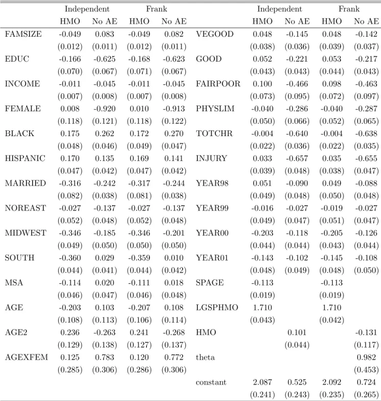
Otherwise, I follow the specification of DMT. In particular, I use the same regressors in the outcome equation. They include indicators of self-perceived health status variables (VEGOOD, GOOD and FAIR-POOR); measures of chronic diseases and physical limitation (TOTCHR, PHYSLIM and INJURY); geo-graphical variables (NOREAST,MIDWEST, SOUTH and MSA); and socio-economic variables (BLACK, HISPANIC, FAMSIZE, FEMALE, MARRIED, EDUC, AGE, AGE2, AGEXFEM and INCOME); respec-tively. I also use the same exclusion restrictions for the insurance choice equations. These are the age of the spouse (SPAGE) and whether the spouse was covered by an HMO in the previous year (LGSPHMO). I refer to DMT for a detailed description of these variables.
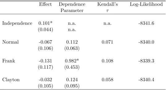
Table 4 contains the key results. For each of the four copulas (independence, normal, Frank and Clayton), it lists the estimated effect of HMO on no ambulatory expenditure, the estimated dependence parameter, Kendall’sτ as well as the log-likelihood value. In this application, the model based on the Frank copula outperforms the other three models. Independence can be formally rejected. The chi-squared (1) - distributed likelihood ratio test statistic is 4.6, withp-value of 0.032 . Similarly, the Frank dependence parameter is significantly smaller than zero. The sign suggests positive self-selection: those who are more likely to opt for HMO have a higher than average probability of having no ambulatory expenses. If unaccounted for, the positive dependence between the unobservables in the two equations is captured by the effect estimate which is indeed found to be positive and even statistically significant in the independence model. Once endogeneity is accounted for, the effect switches its sign and becomes insignificant. In the Frank model, there is no evidence that individuals in an HMO plan have a higher probability of zero ambulatory expenditures than otherwise similar individuals in an PPO plan.
It is interesting to observe that while the point estimates for the effect and dependence parameter under the normal copula assumption are qualitatively similar, the conclusion obtained from formal applications of hypothesis tests would be quite different. Specifically, the independence model cannot be rejected against the bivariate normal model. Likelihood ratio andz-test statistics are both insignificant. As a consequence, one would be led to interpret the +0.1 effect under independence as causal. Under the probit marginals implied by the model, this effect would predict an increase in the probability of no expenditure by up to 4 percentage points, apparently a spurious effect.
The full set of regression coefficients for the independence and Frank copula are displayed in Table 5. Except for the HMO coefficient, there is not much difference between the size and precision of the estimated effects between the two models.
5
Application 2: Dropping out of high school and unemployment
The second application is based on an earlier study by Li (2006) who investigated the effect of high school completion on post-schooling unemployment, accounting for endogeneity of education. Specifically, the analysis was based on data from High School and Beyond, a survey of US high school students (sophomores) in the spring of 1980. Using three follow ups (in 1982, 1984 and 1986) one can determine both whether the student completed high school or not (dropout yes=1) and whether the student had any unemployment experiences upon entering the labor market. Li (2006) also considered the time of drop out (after ninth, tenth or eleventh grade), as well as the intensity of unemployment (proportion of post-school time in unemployment). In the available sample of n = 5238 sophomores, there were 9.5 percent dropouts and 47.1 percent of students with at least one incidence of unemployment.
Clearly, there are many reasons why dropout status and unemployment can be jointly determined, in which case the causal effect of not completing highschool on later unempoloyment cannot be estimated in a simple probit model.Li (2006) used a recursive model structure with bivariate normal assumption to account for endogeneity, plus exclusion restrictions derived from state specific compulsory attendance laws. Using these legal provisions, Li computed for each student in 1980 the variable “Time until eligibility to drop out”. The time depends on the age of the sophomore in 1980 (which is also controlled for) and the state a student lives in. In the sample, 74.7% of the individuals have a compulsory attendance age of 16 or less, 16.5% have a compulsory attendance age of 17, and 8.8% have a compulsory attendance age of 18. Following Li, I use a fourth order polynomial in this time as instrument for actual drop out status. The instrument has some bite. For example, for an average student, increasing the compulsory attendance age from 16 to 18 is predicted to increase the probability of completing high school by 5.1 percentage points. The chi-squared-statistic for the joint significance of the instruments in the dropout equation has ap-value
below 1 %.
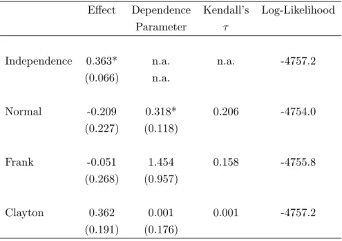
Results are shown in Table 6. In this application, the Normal copula model is clearly the best. The Clayton copula does not work at all, as the estimated dependence parameter is virtually zero, so that this model practically coincides with the independence model, except that the effect is estimated much more imprecisely due to not imposing the zero-dependence restriction. Under both normal and Frank copula, a positive dependence is detected (with estimated Kendall’s τ os 0.21 and 0.16, respectively), but it is statistically significant only in the bivariate probit model. Ignoring the positive correlation between the two errors in the dropout and the unemployment equations causes an upward bias in the effect estimate, as is seen from the first column of Table 6. In fact, there is no longer any statistically significant effect of dropping out on unemployment once endogeneity is accounted for (and the point estimate even turns negative). This result appears to contradict the findings in Li (2006) where dropping out increases the unemployment risk even after accounting for endogeneity. A likely explanation for this discrepancy is that I consider here only the occurrence of any unemployment, whereas Li modeled the severity of it, by using the fraction of time spent in unemployment as outcome variable.
6
Discussion
The paper considered the problem of modeling and estimating the effect of a binary endogenous regressor on a binary outcome variable using a new approach based on copula functions. The copula approach is an alternative to semi-parametric estimation of bivariate probit models (e.g. Murphy, 2007, Chen and Zhou 2007). It offers a relatively simple and parsimonious compromise between the standard bivariate probit model and these semi-parametric alternatives. The main benefits of the copula approach are twofold. First, it makes it relatively effortless to assess the sensitivity of results within a broader class of distribution families. Second, by considering such larger classes of copula families one can obtain, in a quasi-likelihood sense, a better approximation to the true underlying distribution.
The evidence provided in the paper, based on simulations and two real data applications, suggests that copula models work well in practice, and thus provide a viable and simple alternative to the common
bivariate probit approach. Of course, the bivariate probit can well be the best model in the class of copulas that is considered, as was the case in the second application on the effect of completing high school on subsequent unemployment. Even then, however, one does not know this before the analysis is actually completed, and using a menu of copula models provides thus additional information, also on the sensitivity of the estimates to distributional assumptions.
The methods and models presented in the paper have at least two immediate extensions. First, they can be applied to cases where the outcome variable is an ordered response with more than two outcomes. For example, one can easily construct a model with ordered probit marginals for the outcome variable and binary probit marginal for the endogenous regressor. The ordered probit model has a latent variable representation as well. Let
y∗1 =x0β+αy2+ε1
The observed ordered responsesy1 = 1,2, . . . , J are obtained from a threshold observation mechanism
y1 =
J X
j=0
1(y1∗> κj)
whereκs,0=−∞< κs,1 < . . . < κs,J =∞ partition the real line. It follows that
P(y1 =j, y2 = 0) =C(Φ(κj−x0β),Φ(−z0γ))−C(Φ(κj−1−x0β),Φ(−z0γ))
and
P(y1 =j, y2 = 1) =C(Φ(κj−x0β−α),1)−C(Φ(κj−1−x0β−α),1)−P(y1 =j, y2 = 0)
Second, the copula approach can be easily extended to accommodate other marginal models, such as the logit or any other desired link function (Koenker and Yoon, 2009). A bivariate model with logit marginals is obtained by letting F(x, y) =C[Λ(x),Λ(y)], where Λ(z) = exp(z)/(1 + exp(z)) is the cdf of the logistic distribution. Alternatively, one could even estimate the marginals semiparametrically, an approach that has been explored in other copula applications (e.g., Chen and Fan 2005).
A further potentially fruitful development explores copula mixture models, where the underlying joint distribution function of the unobservables is approximated by a finite mixture of parametric distribution
functions that can differ both in their copula specification and in their parameters. Conceptually this is a very elegant approach as it dispenses with the need to select single copulas and moreover can in principle approximate the true joint distribution function to an arbitrary degree. The practical implementation may be very difficult, however, and related results from a study by Trivedi and Zimmer (2009) are not very encouraging.
7
References
Bhattacharya J., D. Goldman and D. McCaffrey (2006) “Estimating Probit Models with Endogenous Covariates,”Statistics in Medicine 25, 389-413.
Chen, X. and Fan, Y. (2005) “Pseudo-likelihood ratio tests for model selection in semiparametric multi-variate copula models”,Canadian Journal of Statistics33, 389 - 414.
Chen, S. and Y. Zhou (2007) “Estimating a generalized correlation coefficient for a generalized bivariate probit model”,Journal of Econometrics141, 1100 - 1114.
Deb, Partha, Murat K. Munkin and Pravin K. Trivedi (2006) “Bayesian Analysis of the Two-Part Model with Endogeneity: Application to Health Care Expenditure”, Journal of Applied Econometrics, 21, 1081-1099.
Evans, W. and R. Schwab (1995) “Finishing High School and Starting College: Do Catholic Schools Make a Difference?”,Quarterly Journal of Economics, 110, 941-974.
Fabbri, D. and C. Monfardini (2008) “Style of practice and assortative mating: a recursive probit analysis of Caesarean section scheduling in Italy,”Applied Economics 40, 1411-1423.
Koenker, R. and J. Yoon (2009) “Parametric links for binary choice models: A Fisherian - Bayesian colloquy”,Journal of Econometrics, forthcoming.
Li, M. (2006) ”High School Completion and Future Youth Unemployment: New Evidence from High School and Beyond”,Journal of Applied Econometrics, 21, 23-53.
Munkin, M.K. and Trivedi, P.K. (2008) “Bayesian Analysis of the Ordered Probit Model with Endogenous Selection”,Journal of Econometrics, 143, 334-348.
Murphy, A. (2007) “Score tests of normality in bivariate probit models”,Economics Letters95, 374 - 379.
Nelson, R.B. (2006) An Introduction to Copulas, Springer, Berlin.
Prokhorov, A. and P. Schmidt (2009) “Likelihood Based Estimation in a Panel Setting: Robustness, Redundancy and Validity of Copulas”,Journal of Econometrics, forthcoming.
Ribar, D.C. (1994) “Teenage Fertility and High School Completion”,Review of Economics and Statistics, 74, 413-424.
Sklar, A. (1959) “Fonctions de r´epartition `a n dimensions et leurs marges”, Publications de l’Institut de Statistique de L’Universit´e de Paris, 8, 229-231.
Smith M.D. (2003) “Modelling sample selection using Archimedean copulas”, Econometrics Journal, 6, 99-123.
Smith M.D. (2005) “Using Copulas to Model Switching Regimes with an Application to Child Labour”,
Economic Record, 81, S47-S57.
Stock, W.A., T.A. Finegan and J.J. Siegfried (2009) “Completing an Economics PhD in Five Years”,
American Economic Review, 99(2), 624-629.
Trivedi, P.K and Zimmer, D.M. (2007) “Copula Modeling: An Introduction for Practitioners”, Founda-tions and Trends in Econometrics, Volume 1, Issue 1.
van Ophem, H. (1999) “A General Method To Estimate Correlated Discrete Random Variables”, Econo-metric Theory, 15, 228-237.
Trivedi, P.K. and D. Zimmer (2009)“Pitfalls in Modeling Dependence Structures: Explorations with Copulas.” Festschrift Volume in Honor of David Hendry, forthcoming.
Van Ophem, H. (2000) “Modeling selectivity in count data model”, Journal of Business and Economic Statistics18, 503-511.
Vella, F. (1999) “Do Catholic Schools Make a Difference? Evidence from Australia”, Journal of Human Resources34, 208-224.
White, H. (1982) “Maximum likelihood estimation of misspecified models”, Econometrica50, 1-26.
Wilde, J. (2000) “Identification of multiple equation probit models with endogenous dummy regressors”,
Economics Letters69, 309-312.
Zimmer, D.M. and Trivedi, P.K. (2006) “Using Trivariate Copulas to Model Sample Selection and Treat-ment Effects: Application to Family Health Care Demand”, Journal of Business and Economic Statistics, 24, 63-76.
Table 1
Simulation Results for Recursive Probit Model with Normal Dependence (ρ= 0.5, r=5000) β0 β1 α θ τ llik % pick n = 500 Normal 0.499 -0.504 0.512 0.497 0.335 -473.5 40.8 (0.107) (0.072) (0.226) (0.132) Frank 0.501 -0.507 0.527 3.419 0.333 -473.7 33.6 (0.108) (0.073) (0.233) (1.251) Clayton 0.467 -0.507 0.554 0.747 0.260 -474.1 25.5 (0.115) (0.074) (0.241) (0.370)
Independence 0.231 -0.527 1.120 n.a. n.a. -479.3 0 (0.086) (0.075) (0.145) n.a. n = 1000 Normal 0.498 -0.502 0.516 0.495 0.332 -949.1 47.5 (0.074) (0.048) (0.157) (0.091) Frank 0.500 -0.504 0.509 3.347 0.332 -949.4 32.7 (0.074) (0.049) (0.162) (0.916) Clayton 0.464 -0.505 0.559 0.707 0.256 -950.3 19.8 (0.080) (0.050) (0.168) (0.241)
Independence 0.230 -0.524 1.121 n.a. n.a. -960.1 0 (0.060) (0.051) (0.101) n.a. n = 5000 Normal 0.500 -0.501 0.500 0.501 0.334 -4763.6 80.0 (0.034) (0.022) (0.071) (0.041) Frank 0.503 -0.504 0.514 3.313 0.333 -4765.2 16.4 (0.034) (0.022) (0.072) (0.367) Clayton 0.465 -0.504 0.546 0.691 0.256 -4769.8 3.6 (0.037) (0.023) (0.075) (0.103)
Independence 0.229 -0.523 1.110 n.a. n.a. -4817.3 (0.027) (0.023) (0.045) n.a.
Notes:
The main entries in the table give the mean values of the statistics over repeated samples. Standard deviations in parentheses.
Table 2
Simulation Results for Recursive Probit Model with Frank Dependence (θ= 3.3,r=5000) β0 β1 α θ τ llik % pick n = 500 Normal 0.492 -0.498 0.503 0.490 0.330 -475.3 28.8 (0.107) (0.072) (0.221) (0.129) Frank 0.501 -0.501 0.503 3.465 0.337 -475.1 52.8 (0.106) (0.072) (0.224) (1.225) Clayton 0.457 -0.500 0.550 0.719 0.252 -476.1 18.4 (0.116) (0.074) (0.240) (0.370)
Independence 0.227 -0.521 1.101 n.a. n.a. -481.0 0 (0.084) (0.075) (0.143) n.a. n = 1000 Normal 0.488 -0.499 0.504 0.492 0.329 -953.7 29.4 (0.074) (0.051) (0.157) (0.091) Frank 0.498 -0.502 0.503 3.404 0.337 -953.4 59.0 (0.074) (0.051) (0.159) (0.811) Clayton 0.451 -0.501 0.555 0.685 0.250 -955.4 11.6 (0.080) (0.052) (0.169) (0.237)
Independence 0.221 -0.521 1.104 n.a. n.a. -964.7 0 (0.059) (0.052) (0.098) n.a. n = 5000 Normal 0.490 -0.497 0.503 0.487 0.324 -4782.3 18.1 (0.034) (0.022) (0.069) (0.040) Frank 0.500 -0.501 0.501 3.309 0.333 -4780.6 81.3 (0.033) (0.023) (0.070) (0.351) Clayton 0.451 -0.499 0.557 0.647 0.243 -4791.0 0.6 (0.037) (0.023) (0.076) (0.100)
Independence 0.225 -0.518 1.095 n.a. n.a. -4833.7 (0.027) (0.023) (0.045) n.a.
Table 3
Simulation Results for Recursive Probit Model with Clayton Dependence (θ= 1,r=5000) β0 β1 α θ τ llik % pick n = 500 Normal 0.513 -0.497 0.521 0.573 0.393 -465.1 19.4 (0.104) (0.072) (0.222) (0.124) Frank 0.507 -0.498 0.551 4.109 0.384 -465.6 9.2 (0.105) (0.073) (0.235) (1.427) Clayton 0.505 -0.501 0.501 1.088 0.341 -464.2 71.4 (0.108) (0.073) (0.222) (0.427)
Independence 0.203 -0.527 1.241 n.a. n.a. -473.0 0 (0.086) (0.076) (0.148) n.a. n = 1000 Normal 0.507 -0.497 0.523 0.574 0.392 -933.7 14.5 (0.072) (0.050) (0.154) (0.086) Frank 0.502 -0.498 0.553 3.750 0.384 -934.9 3.1 (0.073) (0.051) (0.164) (0.834) Clayton 0.499 -0.502 0.502 1.051 0.339 -932.0 82.4 (0.074) (0.050) (0.154) (0.286)
Independence 0.196 -0.526 1.242 n.a. n.a. -949.1 0.0 (0.061) (0.052) (0.099) n.a. n = 5000 Normal 0.509 -0.496 0.522 0.570 0.386 -4681.0 2.0 (0.033) (0.022) (0.070) (0.038) Frank 0.505 -0.498 0.553 3.874 0.378 -4686.6 0.1 (0.033) (0.023) (0.074) (0.403) Clayton 0.500 -0.501 0.501 1.007 0.334 -4672.4 97.9 (0.034) (0.023) (0.070) (0.119)
Independence 0.200 -0.525 1.235 n.a. n.a. -4754.4 (0.027) (0.023) (0.046) n.a.
Table 4: Results for Ambulatory Expenditure Example
Effect Dependence Kendall’s Log-Likelihood
Parameter τ
Independence 0.101* n.a. n.a. -8341.6
(0.044) n.a. Normal -0.067 0.112 0.071 -8340.0 (0.106) (0.063) Frank -0.131 0.982* 0.108 -8339.3 (0.117) (0.453) Clayton -0.032 0.124 0.058 -8340.4 (0.105) (0.095)
Table 5: Full Regression Results for Ambulatory Expenditure
Independent Frank Independent Frank
HMO No AE HMO No AE HMO No AE HMO No AE
FAMSIZE -0.049 0.083 -0.049 0.082 VEGOOD 0.048 -0.145 0.048 -0.142 (0.012) (0.011) (0.012) (0.011) (0.038) (0.036) (0.039) (0.037) EDUC -0.166 -0.625 -0.168 -0.623 GOOD 0.052 -0.221 0.053 -0.217 (0.070) (0.067) (0.071) (0.067) (0.043) (0.043) (0.044) (0.043) INCOME -0.011 -0.045 -0.011 -0.045 FAIRPOOR 0.100 -0.466 0.098 -0.463 (0.007) (0.008) (0.007) (0.008) (0.073) (0.095) (0.072) (0.097) FEMALE 0.008 -0.920 0.010 -0.913 PHYSLIM -0.040 -0.286 -0.040 -0.287 (0.118) (0.121) (0.118) (0.122) (0.050) (0.066) (0.052) (0.065) BLACK 0.175 0.262 0.172 0.270 TOTCHR -0.004 -0.640 -0.004 -0.638 (0.048) (0.046) (0.049) (0.047) (0.022) (0.036) (0.022) (0.035) HISPANIC 0.170 0.135 0.169 0.141 INJURY 0.033 -0.657 0.035 -0.655 (0.047) (0.042) (0.047) (0.042) (0.039) (0.048) (0.038) (0.047) MARRIED -0.316 -0.242 -0.317 -0.244 YEAR98 0.051 -0.090 0.049 -0.088 (0.082) (0.038) (0.081) (0.038) (0.049) (0.048) (0.050) (0.048) NOREAST -0.027 -0.137 -0.027 -0.137 YEAR99 -0.016 -0.027 -0.019 -0.027 (0.052) (0.048) (0.052) (0.048) (0.049) (0.047) (0.051) (0.047) MIDWEST -0.346 -0.185 -0.346 -0.201 YEAR00 -0.203 -0.118 -0.205 -0.126 (0.049) (0.050) (0.050) (0.050) (0.044) (0.044) (0.043) (0.044) SOUTH -0.360 0.029 -0.359 0.010 YEAR01 -0.143 -0.102 -0.145 -0.108 (0.044) (0.041) (0.044) (0.042) (0.048) (0.049) (0.048) (0.050) MSA -0.114 0.020 -0.111 0.018 SPAGE -0.113 -0.113 (0.046) (0.047) (0.046) (0.048) (0.019) (0.019) AGE -0.203 0.103 -0.207 0.108 LGSPHMO 1.710 1.710 (0.108) (0.113) (0.106) (0.114) (0.043) (0.042) AGE2 0.236 -0.263 0.241 -0.268 HMO 0.101 -0.131 (0.129) (0.138) (0.127) (0.137) (0.044) (0.117) AGEXFEM 0.125 0.783 0.120 0.772 theta 0.982 (0.285) (0.306) (0.286) (0.306) (0.453) constant 2.087 0.525 2.092 0.724 (0.241) (0.243) (0.235) (0.265) Standard errors in parentheses; the following variables are scaled by factor 10−1: EDUC, INCOME, AGEXFEM, AGE2.
Table 6: Results for Dropout Example
Effect Dependence Kendall’s Log-Likelihood Parameter τ
Independence 0.363* n.a. n.a. -4757.2 (0.066) n.a. Normal -0.209 0.318* 0.206 -4754.0 (0.227) (0.118) Frank -0.051 1.454 0.158 -4755.8 (0.268) (0.957) Clayton 0.362 0.001 0.001 -4757.2 (0.191) (0.176)
−4 −2 0 2 4 −3 −2 −1 0 1 2 3 v1
Figure 1: 500 draws from a Frank Copula with Standard Normal Marginals, θ= 3.3. Regression line and Locally Weighted Polynomial Regression
−4 −2 0 2 4 −3 −2 −1 0 1 2 3 v1
Figure 2: 500 draws from a Clayton Copula with Standard Normal Marginals, θ= 1. Regression line and Locally Weighted Polynomial Regression
Working Papers of the Socioeconomic Institute at the University of Zurich
The Working Papers of the Socioeconomic Institute can be downloaded from http://www.soi.uzh.ch/research/wp_en.html