Effect of seasonality treatment on the forecasting performance of tourism demand models

Effect of seasonality treatment on the

forecasting performance of tourism

demand models

Institute for Transport Studies, University of Leeds, Leeds LS2 9JT, UK. E-mail: s.shen@its.leeds.ac.uk.

GANG LI

School of Management, University of Surrey, Guildford GU2 7XH, UK. E-mail: g.li@surrey.ac.uk.

HAIYAN SONG

School of Hotel and Tourism Management, Hong Kong Polytechnic University, Hung Hom, Kowloon, Hong Kong, PR China. E-mail: hmsong@polyu.edu.hk.

This study provides a comprehensive comparison of the performance of the commonly used econometric and time-series models in fore-casting seasonal tourism demand. The empirical study is carried out based on the demand for outbound leisure tourism by UK residents to seven destination countries: Australia, Canada, France, Greece, Italy, Spain and the USA. In the modelling exercise, the seasonality of the data is treated using the deterministic seasonal dummies, seasonal unit root test techniques and the unobservable component method. The empirical results suggest that no single forecasting technique is superior to the others in all situations. As far as overall forecast accuracy is concerned, the Johansen maximum likelihood error correction model outperforms the other models. The time-series models also show superior performance in dealing with seasonality. However, the time-varying parameter model performs relatively poorly in forecasting seasonal tourism demand. This empirical evidence suggests that the methods of seasonality treatment affect the fore-casting performance of the models and that the pre-test for seasonal unit roots is necessary and can improve forecast accuracy.

Keywords: seasonality; tourism demand; forecasting; seasonal unit roots; econometric model; time-series model

The work described in this paper was substantially supported by a grant from the Research Grants Council of the Hong Kong Special Administrative Region, China (Project No. PloyU 5473/06H).

T E

Seasonality is one of the most important features of tourism demand and has important impacts on many aspects of the tourism industry. Accurate forecasts of seasonal tourism demand are crucial for the formulation of effective marketing strategies and tourism policies for both the private and public sectors. In addition, seasonality has also been recognized as one of the important tourism research areas (Rodrigues and Gouveia, 2004).

Modelling seasonal variation in international tourism demand has become an important issue in tourism forecasting in recent years (Kulendran and Wong, 2005). However, most previous studies focused only on the time-series methods, such as the seasonal naïve model, the traditional autoregressive integrated moving average (ARIMA) model, the seasonal ARIMA (or SARIMA) model and the basic structural time-series model (BSM) (see, for example, Goh and Law, 2002; Lim and McAleer, 2002; Kulendran and Wong, 2005; Vu, 2006). The augmented BSM with explanatory variables, that is, the multivariate causal structure time-series model (STSM), has also appeared in some published studies that compare the forecasting performance of the above mentioned time-series models (see, for instance, González and Moral, 1995 and 1996; Turner and Witt, 2001). Other econometric techniques, such as the autoregressive distributed lag (ADL) model, the error correction model (ECM), the vector autoregressive (VAR) model and the time-varying parameter (TVP) model, are often omitted from the forecasting competition of seasonal tourism demand models, with only a few exceptions, such as González and Moral (1995), Kulendran and King (1997), Kulendran and Wilson (2000) and Kulendran and Witt (2001, 2003a,b), who compared the forecast accuracy of the ECM with that of the time-series models; Veloce (2004) included both the VAR model and ECM in their forecasting competition, while Smeral and Wüger (2005) examined the forecasting performance of the seasonal naïve, ARIMA, SARIMA and ADL models. It can be seen from these studies that, in seasonal tourism demand forecasting comparisons, only a small number of econometric models (very often one or two only) are selected in the forecasting competition and a predominant focus is often given to the time-series models.

Meanwhile, some efforts have been made in evaluating the forecasting performance of various econometric models as far as annual tourism demand is

concerned, such as Song et al (2003) and Li et al (2006). However, these studies

provided no empirical evidence on the ability of the econometric approaches to deal with seasonality in tourism demand forecasting. There are only a few

exceptions, such as Kulendran and Witt (2001) and Wong et al (2007). In these

comparisons, no more than five forecasting models were included. In particular, one of the most recently developed econometric models – the TVP model – has not been considered. The TVP model has shown its superior performance over the other econometric and time-series models in annual tourism demand forecasting, especially in the short run (see Riddington, 1999; Song and Witt,

2000; Song and Wong, 2003; Song et al, 2003; Li et al, 2006). However, its

performance in seasonal tourism demand forecasting in comparison to other econometric and time-series models has not been examined. An overview of the tourism forecasting literature shows that there has been no systematic comparison across all of the above models regarding their abilities in forecasting seasonal tourism demand.

requires careful treatment in modelling and forecasting seasonal (quarterly or monthly) tourism demand (Kulendran and King, 1997). Kim and Moosa (2001, p 382) noted that, ‘no conclusive evidence was found as to whether one should treat seasonality as stochastic or deterministic’, though the assumption of stochastic seasonality has been popular in recent studies (for example, Lim and McAleer, 2002). Empirical evidence in both tourism (for example, Kim, 1999)

and general economic literatures (for example, Osborn et al, 1999) has suggested

that deterministic seasonality may be more appropriate in modelling and forecasting the seasonal time series. This study will examine this issue further in the tourism demand context.

The primary objective of this study is therefore to bridge the gap in the literature by conducting a comprehensive comparison of the performance of the econometric and time-series models in forecasting seasonal tourism demand. Nine econometric and time-series forecasting models will be included in the forecasting comparison. Particular attention is paid to the performance of the modern econometric models such as the TVP model in dealing with seasonal tourism demand.

Techniques of forecasting seasonal tourism demand

Seasonal time-series forecasting models

Three univariate time-series models are often included in seasonal demand forecasting comparisons: the seasonal naïve model, the SARIMA model and the BSM.

Seasonal naïve model. The seasonal naïve model is normally used to generate baseline forecasts. As far as quarterly data are concerned, the forecast generated

by the seasonal naïve model for the period t + 4 is equal to the value of period

t, that is, F^_t+4 = F_t. For example, forecasts of one and two quarters ahead are

obtained by using the values of the corresponding quarter in the previous year (see Kulendran and Witt, 2001).

SARIMA model. As tourism demand series measured at regular calendar intervals in a year may exhibit periodic behaviour, the general Box–Jenkins

model with seasonal difference (D), seasonal autoregressive term (P) and seasonal

moving average term (Q), can be represented by ARIMA (p, d, q) (P, D, Q)_s:

φp(B)ΦP(B s_)∇d_∇D

sZt = θq(B)ΘQ(B s_)ε

t (1)

where Z_t is a stationary data point at time t, B is the backshift operator, s is

the seasonal periodicity, ε_t is the disturbance at time t, φ_p(B) is the non-seasonal

AR operator, Φ_P(Bs_{) is the seasonal AR operator, θ}

q(B) is the non-seasonal MA

operator, Θ_Q(Bs_{) is the seasonal MA operator, ∇}d _{is the non-seasonal differencing}

operator and ∇D

s is the seasonal differencing operator.

Identification is a critical step in estimating an ARIMA (p, d, q) (P, D, Q)_s

model, where p is the AR order, which indicates the number of parameters of

φ, d is the number of times that the series needs to be differenced in order to

T E

of parameters of θ, P is the seasonal AR order indicating the number of

parameters of Φ, Q is the seasonal MA order indicating the number of

parameters of Θ and D is the number of times that the series needs to be

seasonally differenced to arrive at a seasonally stationary series. However, it is important that the data are properly processed before the estimation takes place, as the ARIMA model requires the time series to be stationary. As most seasonal time series exhibit increasing trend and/or seasonal variations, both seasonal and non-seasonal differencing are often used to achieve a stationary time series.

BSM. A BSM is formulated by decomposing the time series into several

unobservable components as follows:

Y_t = µ_t + γ_t + Ψ_t + ε_t (2)

where Y_t is the actual tourism demand and µ_t, γ_t, Ψ_t and ε_t are the trend,

seasonal, cyclical and irregular components, respectively. Each component of the series can be modelled in several ways (see González and Moral, 1996). With respect to the seasonal component, the trigonometric form is the most commonly used in the literature and will be applied in this empirical study as well. The irregular component represents the transitory variations in tourism demand which cannot be explained by the other components. A particular feature of the BSM is that stochastic movements are permitted. For example, a slowly changing seasonal component may indicate seasonality is stochastic. More details of the BSM specifications can be found in Harvey and Todd (1983).

Econometric models

Five econometric models have been commonly used in the tourism demand forecasting literature and they are the reduced autoregressive distributed lag (RE-ADL) model, the Wickens–Breusch error correction model (WB-ECM), the Johansen maximum likelihood error correction model (JML-ECM), the VAR model and the TVP model. The specifications of these models are available in

Song et al (2003). In addition, the STSM has appeared recently in the seasonal

tourism demand forecasting literature. This model has shown relatively superior forecasting performance, especially when it is compared with ECMs (González and Moral, 1995). Three different techniques are applied to deal with seasonality in this study: the deterministic seasonal dummies, the seasonal unit root test and the unobservable components.

Deterministic seasonal dummies. For the RE-ADL, VAR and TVP models, seasonal dummies are incorporated into the model specifications to capture seasonality. The process generated by the seasonal dummies is normally called a pure deterministic seasonal process. The parameters of the dummies are used to describe the seasonal fluctuations and their effects on the dependent variable.

Normally, s–1 (s is the number of seasons in a one-year cycle, that is,

s = 4 for quarterly time series and s = 12 for monthly data) seasonal dummies are

included in a forecasting model. Seasonal dummies Dit(i = 1,2, . . ., s–1) are

defined as Dit = 1 if time t corresponds to season s and Dit = 0 otherwise. The

use of seasonal dummies implies that the seasonal pattern in a time series Yt

However, Abeysinghe (1994) shows that using the deterministic seasonal dummies in removing seasonality in the time series is likely to result in spurious regressions, as deterministic dummy variables do not reflect the dy-namic nature of the seasonality inherent in the actual tourism demand. If the seasonal effects changed gradually over time, this approach would lead to misspecifications of the dynamic structure of the model because ‘the estimated coefficients on the dummies reflect initial conditions plus the accumulation of random shocks’ (Miron, 1994, p 217). As a result, the forecasts may be biased and can cause inappropriate decision making.

Testing for seasonal unit roots. Although the patterns of seasonality can be deterministic because of the calendar and weather effects, some fluctuations may be caused by the behaviour of tourists and are unlikely to be constant. As Franses (1996, p 299) noted, ‘non-durable consumption patterns may change when preferences for certain holiday seasons change . . . sales can depend upon the state of the economy’. Miron (1994, p 219) argues that ‘it does not make sense to examine estimated seasonal dummy coefficients unless seasonal unit roots can be treated as absent’. A model with seasonal dummies is likely to misrepresent the seasonality as compared with the seasonal integrated process

proposed by Hylleberg et al (1990). A time-series model with seasonal unit roots

is an approximation that allows for changes in the seasonal pattern; that is, the series is integrated at the seasonal frequencies. Such a model is subject to the seasonal unit root test, which involves two steps. The first step is to test for seasonal and non-seasonal unit roots in a time series; and the second step is to apply different seasonal differencing filters to obtain a stationary series before the normal cointegration procedure can be applied to estimate the model, as suggested by the results of the seasonal unit root test. The construction of the WB-ECM and JML-ECM depends on the results of the seasonal unit root test when seasonal data are used in estimating the model.

The HEGY test (Hylleberg et al, 1990) has been commonly used to test for

seasonal and non-seasonal unit roots in a univariate series of a quarterly frequency, and the test is based on the following auxiliary regression:

y_4t = π₁y_1t–1 + π₂y_2t–1 + π₃y_3t–2 + π₄y_3t–1 + ε_t (3) where y_4t = (1–B4_)y t = yt – yt–4 ; y_1t–1 = (1+B+B2_+B3_)y t–1 = yt–1 + yt–2 + yt–3 + yt–4 ; y2t–1 = –(1–B+B2–B3)yt–1 = –(1–B)(1+B2)yt–1 = –yt–1 + yt–2 – yt–3 + yt–4 ; y3t–2 = –(1–B2)yt–2 = –(1–B)(1+B)yt–2 = –yt–2 + yt–4 ; y_3t–1 = –(1–B2_)y t–1 = –yt–1 + yt–3 .

B is the backward shift operator, that is, B(x_t) = x_t–1, and ε_t is a normally and

independently distributed error term with zero mean and constant variance. Deterministic components which include an intercept, three seasonal dummies

T E

and a time trend are also included in Equation (3), which can be estimated by ordinary least squares (OLS). The three null and alternative hypotheses to be tested are as follows:

H₀ : π₁ = 0, H₁ : π₁ < 0 ;

H₀ : π₂ = 0, H₁ : π₂ < 0 ;

H₀ : π₃ = π₄ = 0, H₁ : π₃ ≠ 0 and/or π₄ ≠ 0 .

The HEGY test involves the use of the t-test for the first two hypotheses and

an F-test for the third hypothesis. If the first hypothesis is not rejected, there

is a unit root at the zero frequency, or a non-seasonal unit root in the series. Non-rejection of the second hypothesis implies that there is a seasonal unit root at the semi-annual frequency. Finally, if the third hypothesis is not rejected, there is a seasonal unit root at the annual frequency. These three null hypotheses are tested separately. If none of the three null hypotheses is rejected, a quarterly time series may have non-seasonal, semi-annual and/or annual unit roots. The order of integration of the series would be I(1, 1, 1). The rejection of all three null hypotheses implies that there is no non-seasonal or seasonal unit root, in which case the series is a stationary one and the order of integration of the series would be I(0, 0, 0).

According to the results of the seasonal unit root test, if the order of

integration of the series is I(1, 1, 1), it requires the filters (1 – B), (1 + B)

and (1 + B2_{), respectively, to achieve stationarity. In other words, the seasonal}

differencing filter (1 – B4_{) should be applied to obtain a stationary series. If}

the order of integration is I(0, 0, 0), it implies that the series has deterministic or constant seasonality. In this case, it is sufficient to use dummy variables to capture the seasonal variations in the time series.

Unobservable component. STSM treats seasonality as an unobservable component. Based on the traditional econometric regression model, STSM additionally includes the trend, seasonal, cyclical and irregular components:

Yt = λ1x1 + λ2x2 + . . . + λkxk + µt + γt + Ψt + εt (4)

where Yt is the actual tourism demand, x1,x2,. . .,xk are explanatory variables,

λ1,λ2,. . .,λk are unknown parameters and µt, γt, Ψt, εt are the trend, seasonal,

cyclical and irregular components, respectively. Such a treatment generally assumes that seasonality evolves gradually over time, while the fixed seasonal effect can be embodied in the specifications of the unobservable components as a special case.

The data

The empirical study focuses on the demand for outbound leisure tourism by UK residents to seven major destinations: Australia, Canada, France, Greece, Italy, Spain and the USA. The tourism demand function can be written in the following general form:

TOUit = f(Yt, RRCPit, RSUBit, dummies) (5)

where TOU_it is the UK outbound leisure tourism demand measured by quarterly

tourist arrivals to the destination country i; Y_t is tourist income measured by

real gross domestic product (GDP) of the UK in constant prices (1995 = 100);

RRCP_it represents the relative tourism price of destination i, which is calculated

by dividing the cost of tourism (measured by the consumer price index, CPI_it)

in each destination by the UK CPI (CPI_UK), adjusted by the appropriate

exchange rates (EX_i and EX_UK):

CPI_it/EX_i

RRCP_it = –––––––– (6)

CPIuk/EXuk

RSUB_it represents the relative substitute price of the destination i, measured

by a weighted price index of the main alternative destinations for each of the destinations relative to the tourism price in the UK, with the shares of tourist arrivals in these potential substitute destinations being the weights. For short-haul destinations, the four Western European countries (France, Spain, Greece and Italy) are treated as substitute countries to each other; in the long-haul cases, Australia, Canada and the USA are regarded as substitutes to each other. New Zealand is also added to the long-haul substitution set as it is one of the most popular long-haul destinations for UK tourists. Therefore, Canada, Australia and New Zealand are substitute destinations for the USA; the USA, Australia and New Zealand for Canada; and the USA, Canada and New Zealand for Australia. The reason for choosing these countries as substitutions has been justified by Divisekera (2003). In the case of France, the substitute price is defined as:

RRCP_sp•TOU_sp + RRCP_it•TOU_it + RRCP_gr•TOU_gr

RSUB_fr = ––––––––––––––––––––––––––––––––––––––– (7)

TOUsp + TOUit + TOUgr

Three dummy variables are included in the models to capture the effects of one-off events on the UK outbound tourism demand. Among them, DUM86 represents the severe decline of the world oil prices in 1986 (DUM86 = 1 in 1986Q2 and 1986Q3, 0 otherwise). The severe decline of world oil prices was due to disagreement in the oil cartel (OPEC), which soon led to its breakdown (Trehan, 1986). The decline of world oil prices is supposed to have a positive effect on UK outbound tourism demand. DUM90 captures the effect of the invasion of Kuwait by Iraq in 1990 (DUM90 = 1 in 1990Q3 and 1990Q4, 0 otherwise). DUM91 is used to detect the effects of the Gulf War in 1991 (DUM91 = 1 in 1991Q1, 1991Q2 and 1991Q3, 0 otherwise). These two events may have negative effects on UK outbound tourism demand.

Travel costs between the origin and destination countries may also affect tourism demand to some extent. However, precise measurements of travel costs are rarely available, especially at the aggregate level. The average economy-class airfares between the origin and destination were used to represent travel costs in past studies. However, due to the complex structure of airfares and the low relevance of airfares to the overall price of all-inclusive package tours, only in a few cases did the use of such a proxy result in significant coefficient

T E

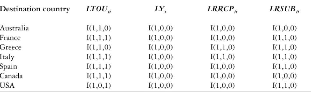
Table 1. Results of unit root tests.

Destination country LTOUit LYt LRRCPit LRSUBit

Australia I(1,1,0) I(1,0,0) I(1,0,0) I(1,0,0) France I(1,1,1) I(1,0,0) I(1,0,0) I(1,1,0) Greece I(1,1,0) I(1,0,0) I(1,1,0) I(1,1,0) Italy I(1,1,1) I(1,0,0) I(1,1,0) I(1,1,0) Spain I(1,1,1) I(1,0,0) I(1,0,0) I(1,1,0) Canada I(1,1,1) I(1,0,0) I(1,0,0) I(1,0,0) USA I(1,0,1) I(1,0,0) I(1,0,0) I(1,1,0)

estimates (Li et al, 2005). Therefore, the travel costs variable is excluded from

this study.

The data cover the period 1984Q1–2004Q4. The series on GDP, exchange

rates and CPI are obtained from the International Financial Statistics Yearbooks

published by the International Monetary Fund (IMF). The tourist arrivals data

are obtained from the Tourism Statistical Yearbooks, published by the United

Nations’ World Tourism Organization (UNWTO).

Empirical results

The six econometric models and three time-series models outlined above are

used to generate individual ex post forecasts. The HEGY test developed by

Hylleberg et al (1990) is used to test for seasonal and non-seasonal unit roots

in the series. The results of unit root tests for the dependent and explanatory variables related to UK tourists to the seven destinations under consideration are presented in Table 1. The tests were carried out for each of the time series for the period 1984Q1–2004Q4 using EVIEWS 5.0.

Performance of the individual forecasting methods

The results of the HEGY test show that the UK outbound tourist arrivals series and some of the price variables exhibit trend and seasonality. The reduced ADL, VAR and TVP models include seasonal dummy variables in the specification of the models to account for deterministic seasonality, while seasonal difference has been used in the WB-ECM and JML-ECM approaches in which seasonality is regarded as stochastic. BSMs and STSMs are estimated using STAMP 7 and the other models are estimated using EVIEW 5.0.

The demand models are estimated based on the data from 1984Q1 to

1996Q4 and the ex post forecasts are generated for the period 1997Q1–2004Q4.1

The recursive forecasting technique is used to generate forecasts; that is, the models are estimated over the period 1984Q1–1996Q4 first and the estimated models are used to forecast tourist arrivals over the period 1997Q1–2004Q4. Subsequently, the models are re-estimated using the data from 1984Q1 to 1997Q1 and forecasts are generated for the period 1997Q2–2004Q4. Such a procedure is repeated until all observations are exhausted. As a result, 32

one-quarter-ahead forecasts, 31 two-quarters-ahead forecasts, 30 three-quarters-ahead forecasts, 29 four-quarters-ahead forecasts and 25 eight-quarters-ahead forecasts are generated. With regard to the SARIMA model, a variety of SARIMA

models with different combinations of the orders of p, q, P, Q are estimated

first and the optimal model is selected based on such information criteria as the Akaike information criterion (AIC) and Schwarz criterion (SC). The orders

of p, q, P and Q are chosen from 0 to 2, according to Pankratz (1983), who

states that in practice, all the orders (p, d, q, P, D, Q) tend to be small, often

no more than 1 or 2 (for SARIMA).

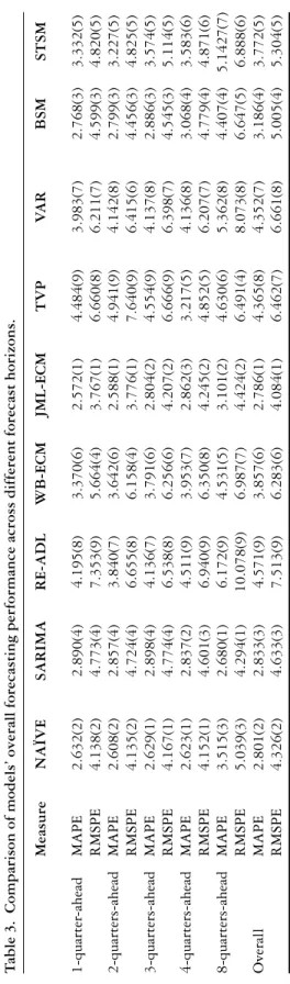
To be consistent with the previous tourism forecasting studies, the forecasting accuracy comparison is carried out based on two measures of error magnitude: the mean absolute percentage error (MAPE) and the root mean square percentage error (RMSPE) (for detailed justification see Witt and Witt, 1992). According to the two error measures, the forecasting performances of the alternative models are ranked and the results are shown in Tables 2 and 3.

Forecasting accuracy comparison across different destinations. The forecast errors of the alternative models for each destination are presented in Table 2. It should be noted that STSM collapses to BSM in four out of seven cases (France, Greece, Italy and the USA), which suggests that after allowing for stochastic determination of the various components of the time series, none of the explanatory variables is statistically significant. The results of Table 2 show that no single model is superior to other techniques across different destinations. For example, the JML-ECM is ranked top overall in terms of both MAPE and RMSPE in the Australia and Greece models. However, the seasonal naïve model outperforms all the other models based on the two measures in the case of France. The WB-ECM is the best performer among all competing models for Italy. With respect to Spain and the USA, the JML-ECM and SARIMA models take alternative turns to be the best based on different error measures.

With respect to the least accurate forecasts, the WB-ECM is outperformed by its competitors in the Australia and Greece cases. The reduced ADL model performs worst in the French and Spanish models according to both error measures. In the USA case, the VAR model exhibits the poorest performance, while for Italy the TVP model produces the least accurate forecasts.

The information above can help forecasters to decide which model to use when forecasting UK tourist arrivals to specific destinations. Although the forecasting performance of the alternative models varies across destinations, the best performing models always treat seasonality as stochastic rather than deterministic with respect to each destination except France. The implication is that, although the demand for tourism to different destinations features different seasonal patterns, to treat seasonality as stochastic is always favourable as far as forecasting the future demand for tourism is concerned.

Forecasting accuracy comparison over different forecast horizons. At each forecast horizon, aggregated error measures are calculated across seven destinations. The results are shown in Table 3. It can be observed from the table that for 1-quarter-ahead and 2-quarters-ahead forecasts, JML-ECM outperforms all the other models in terms of both error measures, followed by the naïve model and BSM. For 3-quarters-ahead and 4-quarters-ahead forecasts, the naïve model

T E

T

able 2.

Comparison of models’ overall forecasting performance across dif

ferent destinations. Destination Measure NAÏVE SARIMA RE-ADL WB-ECM JML-ECM TVP V A R BSM STSM Australia MAPE 4.516(2) 5.048(5) 5.839(6) 7.251(9) 4.130 (1) 6.307 (8) 5.035 (4) 4.710(3) 6.175(7) RMSPE 6.351(2) 7.089(5) 7.711(6) 9.170(9) 5.266(1) 7.839(8) 6.717(4) 6.478(3) 7.819(7) Canada MAPE 3.783(1) 4.147(3) 9.365(7) 4.356(4) 5.322(6) 10.032(8) 10.591(9) 5.237(5) 3.909(2) RMSPE 4.654(1) 5.011(3) 13.112(9) 5.540(4) 6.524(5) 12.011(7) 12.665(8) 7.175(6) 4.745(2) France MAPE 0.932(1) 0.935(2) 2.152(8) 1.067(3) 1.070(4) 1.498(6) 1.559(7) 1.080(5) N/A RMSPE 1.251(1) 1.544(3) 3.540(8) 1.586(4) 1.599(5) 2.023(7) 1.853(6) 1.534(2) N/A Greece MAPE 4.734(2) 5.136(3) 7.506(7) 9.334(8) 4.581(1) 5.252(4) 5.647(5) 5.685(6) N/A RMSPE 7.173(2) 7.756(4) 11.702(7) 12.024(8) 5.727(1) 7.510(3) 8.303(6) 8.081(5) N/A Italy MAPE 2.191(4) 1.963(3) 2.902(7) 1.448(1) 1.818(2) 3.556(8) 2.777(6) 2.221(5) N/A RMSPE 2.783(5) 2.470(3) 3.477(7) 1.925(1) 2.264(2) 4.265(8) 3.460(6) 2.781(4) N/A Spain MAPE 1.193(6) 0.833(1) 1.747(9) 1.537(8) 0.923(3) 1.117(5) 0.918(2) 1.087(4) 1.231(7) RMSPE 1.450(5) 1.213(2) 2.212(9) 2.188(8) 1.156(1) 1.468(6) 1.218(3) 1.362(4) 1.629(7) U S A MAPE 2.261(4) 1.766(2) 2.485(6) 2.010(3) 1.655(1) 2.795(7) 3.939(8) 2.280(5) N/A RMSPE 2.652(3) 2.241(1) 3.052(5) 2.686(4) 2.262(2) 3.379(7) 4.773(8) 3.080(6) N/A Note :

Figures in parentheses indicate the ranks of individual forecasting methods. N/A means the STSM collapses to the BSM in that i

T

able 3.

Comparison of models’ overall forecasting performance across dif

ferent forecast horizons.

Measure NAÏVE SARIMA RE-ADL WB-ECM JML-ECM TVP V A R BSM STSM 1-quarter -ahead MAPE 2.632(2) 2.890(4) 4.195(8) 3.370(6) 2.572(1) 4.484(9) 3.983(7) 2.768(3) 3.332(5) RMSPE 4.138(2) 4.773(4) 7.353(9) 5.664(4) 3.767(1) 6.660(8) 6.211(7) 4.599(3) 4.820(5) 2-quarters-ahead MAPE 2.608(2) 2.857(4) 3.840(7) 3.642(6) 2.588(1) 4.941(9) 4.142(8) 2.799(3) 3.227(5) RMSPE 4.135(2) 4.724(4) 6.655(8) 6.158(4) 3.776(1) 7.640(9) 6.415(6) 4.456(3) 4.825(5) 3-quarters-ahead MAPE 2.629(1) 2.898(4) 4.136(7) 3.791(6) 2.804(2) 4.554(9) 4.137(8) 2.886(3) 3.574(5) RMSPE 4.167(1) 4.774(4) 6.538(8) 6.256(6) 4.207(2) 6.666(9) 6.398(7) 4.545(3) 5.114(5) 4-quarters-ahead MAPE 2.623(1) 2.837(2) 4.511(9) 3.953(7) 2.862(3) 3.217(5) 4.136(8) 3.068(4) 3.583(6) RMSPE 4.152(1) 4.601(3) 6.940(9) 6.350(8) 4.245(2) 4.852(5) 6.207(7) 4.779(4) 4.871(6) 8-quarters-ahead MAPE 3.515(3) 2.680(1) 6.172(9) 4.531(5) 3.101(2) 4.630(6) 5.362(8) 4.407(4) 5.1427(7) RMSPE 5.039(3) 4.294(1) 10.078(9) 6.987(7) 4.424(2) 6.491(4) 8.073(8) 6.647(5) 6.888(6) Overall MAPE 2.801(2) 2.833(3) 4.571(9) 3.857(6) 2.786(1) 4.365(8) 4.352(7) 3.186(4) 3.772(5) RMSPE 4.326(2) 4.633(3) 7.513(9) 6.283(6) 4.084(1) 6.462(7) 6.661(8) 5.005(4) 5.304(5) Note :

T E

generates the most accurate forecasts, followed by JML-ECM. The BSM and SARIMA models generate more accurate forecasts than the rest of the models. For 8-quarters-ahead forecasts, the SARIMA model turns out to be the top-performing model, followed by JML-ECM and the naïve model in terms of both error measures. The reduced ADL model and the VAR model perform consistently poorly over different forecast horizons and are ranked among the bottom three. The TVP model produces the least accurate forecasts for the short forecast horizons (1-, 2- and 3-quarters-ahead); however, slightly better performance is observed for the longer forecast horizons. BSM outperforms STSM for all forecast horizons, which suggests that inclusion of explanatory variables does not seem to improve the forecast accuracy of the structural time-series model. This result is in line with the findings of previous studies, such as Turner and Witt (2001).

The results highlighted above show that for short-term (one to two steps ahead) forecasting, JML-ECM performs the best, which indicates that by incorporating the short-run dynamics into the econometric modelling procedure, the forecasting accuracy can be improved. However, the naïve model and the BSM still outperform the other models, although they do not perform as well as the JML-ECM. For medium-term forecasting (three and four steps ahead), the naïve model generates the most accurate forecasts, followed by JML-ECM. As far as the long-run forecasts are concerned, the SARIMA model outperforms all of its counterparts, closely followed by the JML-ECM and the naïve model. It is clear from the above analysis that the econometric models outperform the time-series models in the short run, while the time-series models are more accurate in the medium- to long-run forecasting.

Overall forecasting accuracy. The bottom rows of Table 3 present the aggregated accuracy measures across all destinations and over all forecast horizons. The results show that JML-ECM is superior to all other models when forecasting UK outbound tourist arrivals to the seven major destination countries. The results are contradictory to the conclusions drawn in previous studies (such as Kulendran and King, 1997; Kulendran and Witt, 2001) in which the econometric models are outperformed by simple univariate time-series models. The time-series models perform well and rank second (the naïve model) and third (the SARIMA model), respectively. The reduced ADL model generates the least accurate forecasts, while the TVP model (or the VAR model) produces the second least accurate forecasts based on either MAPE or RMSPE.

The superior performances of JML-ECM and the seasonal time-series models might be explained by the way in which the seasonality in the data series is treated. The nature of seasonality in the time series is regarded as either deterministic or stochastic. When seasonality is stochastic, the time series needs to be seasonally differenced to account for seasonal unit roots. If seasonality is found to be deterministic, seasonal dummies could be used to capture seasonality in the model. The specifications of JML-ECM and WB-ECM are based on the results of the seasonal unit root test (HEGY hereby). The seasonal naïve model and the SARIMA model assume that there are seasonal unit roots at seasonal frequencies, while this assumption is consistent with the results of the seasonal HEGY test, which indicate that UK outbound tourist arrivals exhibit stochastic seasonality. By including stochastic seasonality as

one of the main components, BSM and STSM allow for changing seasonal patterns in tourism demand. However, the other three models use seasonal dummies to account for seasonality in tourism demand. According to Abeysinghe (1994), the use of seasonal dummies in removing seasonality in the data is likely to produce spurious regressions. Moreover, such a simplification is incapable of reflecting the dynamic nature of the seasonality in tourism demand. Moosa and Kennedy (1998) draw a similar conclusion. That may also explain the relatively poor forecasting performances of the reduced ADL, VAR and TVP models.

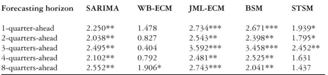
It is necessary to examine the statistical significance of the forecast differences between the above two groups of forecasting models, that is, JML-ECM, WB-ECM, STSM, BSM and the SARIMA model, which all treat seasonality as stochastic, and the reduced ADL, VAR and TVP models, which assume deterministic seasonality. The Harvey–Leybourne–Newbold (HLN) test

proposed by Harvey et al (1997) is adopted for this purpose. The HLN test is

a modified version of the Diebold and Mariano (1995) test and is suitable for small samples and multiple-step-ahead forecasts. The technical illustration of

the statistic is omitted here as it can be found in Harvey et al (1997). The results

of the tests are reported in Tables 4–6. The evidence clearly suggests that treating seasonality as a stochastic process can improve forecast accuracy significantly. The JML-ECM, WB-ECM, BSM, STSM and ARIMA models outperform the reduced ADL, VAR and TVP models significantly in 70% of the comparisons, with only WB-ECM showing relatively less satisfactory performance.

A significant contribution of this study is that it has confirmed that different treatments of seasonality can affect the forecasting performance of the tourism demand forecasting models significantly and pre-tests for seasonal unit roots can improve forecast accuracy. This finding is consistent with Alleyne (2006) and Diebold and Kilian (2000).

Conclusions

This study has provided a comprehensive comparison of the forecasting performance of six econometric models and three time-series models related to UK outbound tourism demand. The econometric models comprise a reduced ADL model, two ECMs (WB-ECM and JML-ECM), an unrestricted VAR model, a TVP model and an STSM. Five of these models represent the latest developments of econometric modelling and forecasting methods in the tourism context and have shown their advantages over the other models in previous empirical studies. The time-series models include a naïve model, a SARIMA model and a BSM. These time-series models have been used widely in modelling seasonal time series.

As quarterly data were used in this study, three methods were used to treat seasonality in the econometric modelling process – using seasonal dummies, testing for seasonal roots (seasonal differencing) and decomposing the unobservable components. The HEGY unit root test was employed to test for the nature of seasonality in the time series. The forecasting accuracy of the different forecasting techniques was compared based on two error magnitude measures,

T E

Table 4. Tests for equal forecast accuracy between RE-ADL model and other models with stochastic seasonality.

Forecasting horizon SARIMA WB-ECM JML-ECM BSM STSM

1-quarter-ahead 2.250** 1.478 2.734*** 2.671*** 1.939* 2-quarters-ahead 2.038** 0.827 2.543** 2.398** 1.795* 3-quarters-ahead 2.495** 0.404 3.592*** 3.458*** 2.452** 4-quarters-ahead 2.102** 0.792 2.481** 2.525** 1.631 8-quarters-ahead 2.552** 1.906* 2.743*** 2.041** 1.437

Note: *, ** and *** represent 10%, 5% and 1% significant levels, respectively.

Table 5. Tests for equal forecast accuracy between TVP model and other models with stochastic seasonality.

Forecasting horizon SARIMA WB-ECM JML-ECM BSM STSM

1-quarter-ahead 3.945*** 1.736* 5.778*** 5.976*** 4.909*** 2-quarters-ahead 4.338*** 2.210** 5.932*** 5.414*** 4.851*** 3-quarters-ahead 2.758*** 0.450 3.920*** 3.760*** 2.915*** 4-quarters-ahead 0.289 –1.955* 0.591 0.214 0.736 8-quarters-ahead 2.592** –0.421 2.440** –0.118 0.556

Note: *, ** and *** represent 10%, 5% and 1% significant levels, respectively. The negative statistics suggest that the TVP model outperforms its competitors.

Table 6. Tests for equal forecast accuracy between VAR model and other models with stochastic seasonality.

Forecasting horizon SARIMA WB-ECM JML-ECM BSM STSM

1-quarter-ahead 2.838*** 0.836 4.328*** 5.116*** 3.975*** 2-quarters-ahead 2.750*** 0.552 4.342*** 4.154*** 3.110*** 3-quarters-ahead 2.536** 0.169 3.594*** 3.799*** 2.540** 4-quarters-ahead 2.034** 0.072 2.590** 2.624*** 1.857* 8-quarters-ahead 1.939* 0.654 1.916* 1.569 0.931

Note: *, ** and *** represent 10%, 5% and 1% significant levels, respectively.

that is, the MAPE and RMSPE. Rankings of these forecasting models over different time horizons were provided.

The empirical results have shown that no single forecasting technique is superior to the others in all situations as the performance of tourism forecasting models tends to vary across destinations and forecast horizons. This finding is in line with previous studies (for example, Fildes and Lusk, 1984; Makridakis,

1986; Wong et al, 2007).

With regard to the overall performance of the models in forecasting seasonal tourism demand, the results show that JML-ECM is superior to all other models, followed by the simple naïve model and the SARIMA model. BSM

outperforms STSM, suggesting that the inclusion of explanatory variables does not seem to improve the forecast accuracy of the basic structural time-series model. The ADLM, VAR and TVP models, which include seasonal dummies to account for seasonality, performed relatively poorly as compared with the other models. This empirical evidence suggests that different treatment of seasonality affects the forecasting performance of the econometric models. When seasonality is regarded as stochastic, the time series needs to be seasonally differenced, or seasonality should be treated as a stochastic component to account for seasonal unit roots in the time series. To model seasonality as a deterministic component by using seasonal dummies may result in model misspecification. Therefore, the test for seasonal unit roots before estimating the model is necessary and can improve forecast accuracy.

Although the applications of the TVP model have shown its superiority in tourism demand forecasting as far as annual data are concerned, its performance has been unsatisfactory when quarterly data are used and only deterministic seasonal dummies are introduced. As the time-series models employed in this study can treat seasonality as a stochastic component using BSM, the combination of the TVP model and the BSM might improve the forecasting performance with higher frequency data (monthly or quarterly). Further research in this respect would certainly be of interest to both researchers and practitioners.

Endnotes

1. The results are omitted here due to space constraints but are available from the authors on request.

References

Abeysinghe, T. (1994), ‘Deterministic seasonal models and spurious regressions’, Journal of Econometrics, Vol 61, pp 259–272.

Alleyne, D. (2006), ‘Can seasonal unit root testing improve the forecasting accuracy of tourist arrivals?’, Tourism Economics, Vol 12, pp 45–64.

Diebold, F.X., and Kilian, L. (2000), ‘Unit root tests are useful for selecting forecasting models’,

Journal of Business and Economic Statistics, Vol 18, pp 265–273.

Diebold, F.X., and Mariano, R.S. (1995), ‘Comparing predictive accuracy’, Journal of Business and Economic Statistics, Vol 13, pp 253–263.

Divisekera, S. (2003), ‘A model of demand for international tourism’, Annals of Tourism Research, Vol 30, pp 31–49.

Fildes, R., and Lusk, E.J. (1984), ‘The choice of a forecasting model’, OMEGA, Vol 12, pp 427– 435.

Franses, P.H. (1996), ‘Recent advances in modelling seasonality’, Journal of Economic Survey, Vol 10, pp 299–345.

Goh, C., and Law, R. (2002), ‘Modelling and forecasting tourism demand for arrivals with stochastic non-stationary seasonality and intervention’, Tourism Management, Vol 23, pp 499–510. González, P., and Moral, P. (1995), ‘An analysis of the international tourism demand in Spain’,

International Journal of Forecasting, Vol 11, pp 233–251.

González, P., and Moral, P. (1996), ‘Analysis of tourism trends in Spain’, Annals of Tourism Research, Vol 23, pp 739–754.

Harvey, A.C., and Todd, P.H.J. (1983), ‘Forecasting economic time series with structural and Box– Jenkins models: a case study’, Journal of Business and Economic Statistics, Vol 1, pp 299–307. Harvey, D., Leybourne, S., and Newbold, P. (1997), ‘Testing the equality of prediction mean squared

errors’, International Journal of Forecasting, Vol 13, pp 281–291.

Hylleberg, S., Engle, R.F., Granger, C.W.J., and Yoo, B.S. (1990), ‘Seasonal integration and cointegration’, Journal of Econometrics, Vol 44, pp 215–238.

T E

Kim, J.H. (1999), ‘Forecasting monthly tourist departures from Australia’, Tourism Economics, Vol 5, pp 277–291.

Kim, J.H., and Moosa, I. (2001), ‘Seasonal behaviour of monthly international tourist flows: specification and implications for forecasting models’, Tourism Economics, Vol 7, pp 381–396. Kulendran, N., and King, M. (1997), ‘Forecasting international quarterly tourism flows using error

correction and time series models’, International Journal of Forecasting, Vol 13, pp 319–327. Kulendran, N., and Wilson, K. (2000), ‘Modelling business travel’, Tourism Economics,Vol 6, pp 47–

59.

Kulendran, N., and Witt, S.F. (2001), ‘Cointegration versus least squares regression’, Annals of Tourism Research, Vol 28, pp 291–311.

Kulendran, N., and Witt, S.F. (2003a), ‘Forecasting the demand for international business tourism’,

Journal of Travel Research, Vol 41, pp 265–271.

Kulendran, N., and Witt, S.F. (2003b), ‘Leading indicator tourism forecasts’, Tourism Management, Vol 24, pp 503–510.

Kulendran, N., and Wong, K.K.F. (2005), ‘Modelling seasonality in tourism forecasting’, Journal of Travel Research, Vol 44, pp 163–170.

Li, G., Song, H., and Witt, S.F. (2005), ‘Recent development in econometric modelling and forecasting’, Journal of Travel Research, Vol 44, pp 82–99.

Li, G., Wong, K.F., Song, H., and Witt, S.F. (2006), ‘Tourism demand forecasting: a time varying parameter error correction model’, Journal of Travel Research, Vol 45, pp 175–185.

Lim, C., and McAleer, M. (2002), ‘Time series forecasts of international travel demand for Australia’,

Tourism Management, Vol 23, pp 389–396.

Makridakis, S. (1986), ‘The art and science of forecasting: an assessment and future directions’,

International Journal of Forecasting, Vol 2, pp 15–29.

Miron, J.A. (1994), ‘The economics of seasonal cycles’, in Sims, C.A., ed, Advances in Econometrics,

Sixth World Congress of the Econometric Society, Cambridge University Press, Cambridge. Moosa, I.A., and Kennedy, P. (1998), ‘Modelling seasonality in the Australian consumption function’,

Australian Economic Papers, Vol 37, pp 88–102.

Osborn, D.R., Harevi, S., and Birchenhall, C.R. (1999), ‘Seasonal unit roots and forecasts of two-digit European industrial production’, International Journal of Forecasting, Vol 15, pp 27–47. Pankratz, A. (1983), Forecasting with Univariate Box–Jenkins Models, Wiley, New York.

Riddington, G. (1999), ‘Forecasting ski demand: comparing learning curve and time varying parameter approaches’, Journal of Forecasting, Vol 18, pp 205–214.

Rodrigues, P.M.M., and Gouveia, P.M.D.C.B. (2004), ‘An application of PAR models for tourism forecasting’, Tourism Economics, Vol 10, pp281–303.

Smeral, E., and Wüger, M. (2005), ‘Does complexity matter? Methods for improving forecasting accuracy in tourism: the case of Australia’, Journal of Travel Research, Vol 44, pp 100–110. Song, H., and Witt, S.F. (2000), Tourism Demand Modelling and Forecasting: Modern Econometric

Approaches, Pergamon, Cambridge.

Song, H., and Wong, K.K.F. (2003), ‘Tourism demand modelling: a time-varying parameter approach’,Journal of Travel Research, Vol 42, pp 57–64.

Song, H., Witt, S.F., and Jensen, T.C. (2003), ‘Tourism forecasting: accuracy of alternative econometric models’, International Journal of Forecasting, Vol 19, pp 123–141.

Trehan, B. (1986), ‘Oil prices, exchange rates and the US economy: an empirical investigation’,

Economic Review, Federal Reserve Bank of San Francisco, Vol 4, pp 25–43.

Turner, L.W., and Witt, S.F. (2001), ‘Forecasting tourism using univariate and multivariate structural time series models’, Tourism Economics, Vol 7, pp 135–147.

Veloce, W. (2004), ‘Forecasting inbound Canadian tourism: an evaluation of error corrections model forecasts’, Tourism Economics, Vol 10, pp 263–280.

Vu, C.J. (2006), ‘Effect of demand volume on forecasting accuracy’, Tourism Economics, Vol 12, pp 263–276.

Witt, S.F., and Witt, C.A. (1992), Modelling and Forecasting Demand in Tourism, Academic Press, London.

Wong, K.K.F., Song, H., Witt, S.F., and Wu, D.C. (2007), ‘Tourism forecasting: to combine or not to combine?’, Tourism Management, Vol 28, pp 1068–1078.