Fakultät/ Zentrum/ Projekt XY Institut/ Fachgebiet YZ
07-2018
Institute of Economics
Hohenheim Discussion Papers in Business, Economics and Social Sciences
TESTING FOR COINTEGRATION WITH
THRESHOLD ADJUSTMENT IN THE
PRESENCE OF STRUCTURAL BREAKS
Karsten Schweikert
Discussion Paper 07-2018
Testing for cointegration with t
h
reshold adjustment in the
presence of structural breaks
Karsten Schweikert
Download this Discussion Paper from our homepage:
https://wiso.uni-hohenheim.de/papers
ISSN 2364-2084
Die Hohenheim Discussion Papers in Business, Economics and Social Sciences dienen der schnellen Verbreitung von Forschungsarbeiten der Fakultät Wirtschafts- und Sozialwissenschaften.
Die Beiträge liegen in alleiniger Verantwortung der Autoren und stellen nicht notwendigerweise die Meinung der Fakultät Wirtschafts- und Sozialwissenschaften dar.
Hohenheim Discussion Papers in Business, Economics and Social Sciences are intended to make results of the Faculty of Business, Economics and Social Sciences research available to the public in
order to encourage scientific discussion and suggestions for revisions. The authors are solely responsible for the contents which do not necessarily represent the opinion of the Faculty of Business,
Testing for cointegration with threshold adjustment
in the presence of structural breaks
Karsten Schweikert
∗University of Hohenheim
Abstract
In this paper, we develop new threshold cointegration tests with SETAR and MTAR adjustment allowing for the presence of structural breaks in the equi-librium equation. We propose a simple procedure to simultaneously estimate the previously unknown breakpoint and test the null hypothesis of no cointegra-tion. Thereby, we extend the well-known residual-based cointegration test with regime shift introduced by Gregory and Hansen(1996a) to include forms of non-linear adjustment. We derive the asymptotic distribution of the test statistics and demonstrate the finite-sample performance of the tests in a series of Monte Carlo experiments. We find a substantial decrease of power of the conventional threshold cointegration tests caused by a shift in the slope coefficient of the equi-librium equation. The proposed tests perform superior in these situations. An application to the ‘rockets and feathers’ hypothesis of price adjustment in the US gasoline market provides empirical support for this methodology.
Keywords: Cointegration, threshold autoregression, structural breaks, SETAR, MTAR, asymmetric price transmission
MSC Codes: 62H15, 62M10, 62P20
JEL Codes: C12, C32, C34, Q41
∗Address: University of Hohenheim, Department of Econometrics and Statistics, Schloss
Hohen-heim 1 C, 70593 Stuttgart, Germany, telephone: (0711) 459-24713, e-mail: [email protected]
1
Introduction
The residual-based threshold cointegration models developed by Enders and Siklos
(2001) are a useful addition to the toolbox of researchers working with multivariate time series. They are easy to apply, allow for discontinuous adjustment to a long-run equilibrium and nest linear cointegration in the sense of Engle and Granger (1987) as a special case. The dynamics of the adjustment process are described by a two-regime threshold autoregressive (TAR) model which partitions the residual process according to a threshold value and specifies different coefficients of the leading autoregressive lag for each regime. It can therefore be considered a restricted model under the general class of TAR models described by Tong (1983, 1990). A prominent application in the economics literature is the empirical analysis of asymmetric price transmissions in which case non-stationary price series form a cointegrating relationship and may feature asym-metric adjustment to long-run equilibrium. The speed of adjustment is usually assumed to depend on the sign and magnitude of the deviations from the long-run equilibrium. While threshold cointegration models are suitable to study these cases, they do not account for possible structural change in the long-run relationship. It is well-known that conventional residual-based cointegration tests perform poorly when a cointegra-tion relacointegra-tionship has structural breaks (see, for example,Gregory et al. (1996)). Maki
(2012) found that the power property of threshold cointegration tests is more robust to structural breaks than, for example, the Engle-Granger cointegration tests assuming linear adjustment. Nevertheless, the power of all residual-based cointegration tests is impaired if the tests do not model the structural breaks explicitly. Consequently, it is difficult to provide evidence for the existence of a cointegration relationship. Further-more, the estimated adjustment coefficients are biased if the cointegrating vector does not account for structural change.
An extensive body of literature exists on the problem of structural instability in time series. Based on the seminal work of Perron (1989), several unit root tests ac-counting for structural change have been developed (see, inter alia,Zivot and Andrews
(1992),Lumsdaine and Papell(1997) andLee and Strazicich(2003)). Structural breaks in linear cointegration models are addressed in Gregory and Hansen (1996a,b), Arai and Kurozumi (2007),Carrion-i Silvestre and Sanso (2006), Westerlund and Edgerton
(2007) andHatemi-J (2008). For a comprehensive survey on structural change in time series models, seePerron(2006). Gregory and Hansen(1996a), henceforth GH, propose a residual-based cointegration test with structural break. Their test does not require
a pre-specified breakpoint which is rarely known in empirical applications. Instead, a single unknown breakpoint is determined from the data based on one of three struc-tural break models. However, the GH test is only suitable for cointegration models with linear adjustment.1 We contribute to the literature by extending the GH test to include two forms of non-linear adjustment. These new tests are residual-based and use either a self-exciting threshold autoregressive (SETAR) model or a momentum thresh-old autoregressive (MTAR) to describe the adjustment toward equilibrium. Thereby, we also provide an extension to the Enders-Siklos cointegration tests which are robust to a structural break in the cointegrating vector.
We derive the limiting distributions of the test statistics considered in this paper and provide a formal proof. The properties of the proposed test are investigated by Monte Carlo experiments for a variety of models ranging from linear adjustment with no structural break to non-linear adjustment with structural break in the intercept and slope coefficients. The results suggest that a break in the intercept does not influence the power of the threshold cointegration tests enough to justify modelling the structural break. However, a break in the slope coefficients reduces the power of the Enders-Siklos tests substantially such that our proposed tests perform clearly better than their bench-marks. In addition, we find that the unknown breakpoints are estimated accurately by the new procedure.
The methodology is applied to empirical data in the context of the ‘rockets and feathers’ hypothesis. We use US gasoline market data covering the Financial Crisis. We illustrate that empirical evidence for the existence of a long-run relationship between neighbouring stages of the gasoline value-chain can only be provided if we control for a structural break in the cointegrating vector. Using a cointegration model with SETAR adjustment and the possibility of structural breaks, we find evidence for asymmetric adjustment from spot gasoline to retail gasoline prices. The MTAR model yields similar results.
The paper is organized as follows. Section 2 describes the models and the cointe-gration testing procedure, Section 3 presents the asymptotic distributions of the test statistics. Section 4 is devoted to the Monte Carlo simulation study. Section 5 reports the results of the empirical application, and Section 6 summarizes the study.
1The effects on the power properties of linear cointegration tests, if the equilibrium error follows a
2
Models and cointegration testing
The long-run equilibrium equation of Engle-Granger cointegration models is given by
yt = µ+α1x1t+α2x2t+· · ·+αmxmt+et
= µ+α0xt+et (1)
where t = 1,2, . . . , T is the time series index, yt and xt = (xit, x2t, . . . , xmt)0 are I(1)
variables, µ is an intercept, α0 = (α1, α2, . . . , αm) is a vector of slope coefficients and
et is the equilibrium error. The null hypothesis of no cointegration is rejected if the
residuals obtained from least squared estimation of (1) are mean-zero stationary. Since the parametersµand αare time-invariant, a residual-based cointegration test based on (1) becomes invalid if the long-run equilibrium is subject to structural change.
FollowingPerron (1989) and Gregory and Hansen(1996a), we consider three forms of structural change.2 First, in the C model, a break in the intercept µ is considered. This model captures events that cause a parallel shift of the equilibrium equation. Second, the C/T model adds an additional trend term to the equilibrium equation. Third, in theC/S model, a simultaneous break in the constant and slope parameters is specified. This model allows for the possibility of a complete regime shift at one point in time. The three models are given as follows,
(C) yt = µ1+µ2ϕt,τ +α0xt+etτ
(C/T) yt = µ1+µ2ϕt,τ +δt+α0xt+etτ (2)
(C/S) yt = µ1+µ2ϕt,τ +α01xt+α02xtϕt,τ +etτ
where µ1, µ2 are constants, α1 = (α11, α12, . . . , α1m)0 and α2 = (α21, α22, . . . , α2m)0 are
slope coefficients. The dummy variableϕt,τ is defined as
ϕt,τ = 1 if t ≥[T τ] 0 if t <[T τ] , (3)
where τ ∈(0,1) denotes the relative timing of the breakpoint (break fraction), and [·] denotes integer part. The timing of the breakpoint is rarely known in empirical
applica-2We restrict our analysis to these three models. However, our methodology can easily be adapted
for other structural break models, as for example given inGregory and Hansen(1996b) andHatemi-J
tions so that the GH test is constructed without the need of pre-specified breakpoints. More specifically, a grid search over all possible breakpoint is employed, i.e. the struc-tural change model is repeatedly estimated for each possible break fractionτ ∈ T. The setT can be any compact subset of (0,1) which excludes endpoint results. GH suggest a lateral trimming of 15 percent (T = (0.15,0.85)) and, for computational reasons, consider only integer steps. Estimating one of the structural break models in (3) by least squares for each breakpoint yields a sequence of residuals. The GH test applies the ADF test to each sequence and evaluates the null hypothesis of no cointegration based on the smallest values of thet ratios across all τ ∈ T. The infimum statistic is chosen since it puts the most weight on the alternative hypothesis. If the null hypothesis is rejected, the break fraction ˆτ corresponding to the infimum statistic is considered to be the most likely breakpoint.
In order to account for asymmetric adjustment, the two-regime SETAR model is now used to describe the adjustment toward equilibrium. The SETAR model for the breakpoint-specific equilibrium error processetτ is given by
∆etτ =ρ1et−1τ1{et−1τ ≥λ}+ρ2et−1τ1{et−1τ < λ}+ K
X
j=1
γj∆et−jτ +tτ K, (4)
where1{·}denotes the Heaviside indicator function, the parameterλis a possibly non-zero threshold value and tτ K is a stationary mean zero error term. The coefficient ρ1 measures the mean-reversion toward the attractor after a shock greater than or equal to λ whereas ρ2 measures the mean-reversion toward the cointegrating vector after a shock less than λ. The indicator function in this case is set according to the level of
et−1τ.
In an alternative specification, suggested byEnders and Granger (1998) and Caner and Hansen(2001), the indicator function is set depending on ∆et−1τ. The two-regime
MTAR model is given by
∆etτ = ρ1et−1τ1{∆et−1τ ≥λ}+ρ2et−1τ1{∆et−1τ < λ}+ K
X
j=1
γj∆et−jτ +tτ K.
In this specification,ρ1measures the mean-reversion toward the attractor if a shock has momentum greater than or equal toλ whereasρ2 measures the mean-reversion toward the cointegrating vector if a shock has momentum less thanλ.
process (DGP) of etτ is symmetric and a unit root is present in both regimes. Models
(4) and (5) are a special case of the general class of threshold autoregressive models in that they do not allow for regime-specific deterministic terms and regime-specific dynamics beyond the leading autoregressive lag. This restriction is convenient since it circumvents the problem of having an identified threshold under the null hypothesis resulting in an asymptotic distribution of the test statistic that depends on nuisance parameters (seeCaner and Hansen(2001) for a more detailed discussion in the context of MTAR processes with a unit root). Furthermore, the Engle-Granger test for symmetric adjustment (ρ1 = ρ2) is itself a special case of (4) and (5). Petruccelli and Woolford (1984) show that the stationarity of the SETAR process is ensured if ρ1 < 0, ρ2 < 0 and (1 +ρ1)(1 +ρ2) < 1 for any value λ. In the case of MTAR processes, Lee and
Shin (2000) prove that stationarity is ensured if ρ1 < 0, ρ2 < 0, (1 +ρ1)(1 +ρ2) < 1, (1+ρ1)(1+ρ2)2 <1 and (1+ρ1)2(1+ρ2)<1. Assuming stationarity,Tong(1983,1990) demonstrated that least squares estimators of ρ1 and ρ2 are asymptotically normally distributed. Enders and Siklos (2001) recommend a Wald-type F-test to test the null hypothesis of no cointegration in their model without structural breaks. However, since the F-test can lead to rejection of the null hypothesis when only one coefficient is negative, the test should only be applied if both point estimates suggest a mean-reversion behaviour. In other words, the one-sided alternative ρ1 < 0∧ρ2 ≥ 0 or
ρ2 <0∧ρ1 ≥0 should not lead to rejection of the null hypothesis.
In the case of a cointegration model with potential structural break, we propose the following cointegration test: First, an appropriate structural break model is selected from (3) and the cointegrating regression is estimated by least squares for each break fraction τ ∈ T. Then, the SETAR or MTAR regression is estimated and the F -statistic, Fτ, is computed for each sequence of residuals. Since the null hypothesis of
no cointegration is naturally rejected for large values of theF-statistic, the supremum statistic,
F∗ = sup
τ∈T
Fτ, (5)
is used to evaluate the null hypothesis of no cointegration against the alternative of threshold cointegration with possible structural break. The largest value found in this grid search also determines the most likely breakpoint.
3
Asymptotic distribution
In the following, we present the asymptotic distributions of the test statistics as func-tionals of Brownian motion. The asymptotic theory for SETAR processes with a unit root was developed inSeo(2008) and the asymptotic theory for MTAR processes with a unit root was developed inCaner and Hansen(2001). Gregory and Hansen(1996a) pro-vide important results for cointegration test statistics which are functions of the break fraction parameterτ and serves as the building block for our residual-based tests.
For notational convenience we use ‘⇒’ to signify weak convergence of the associated probability measures. Continuous stochastic processes such as the Brownian motion
B(s) on [0,1] are simply written as B if no confusion will be caused. We also write integrals with respect to the Lebesgue measure such as
1 R 0 B(s)ds simply as 1 R 0 B.
Let{zt}∞0 be an (m+ 1)-vector integrated process whose data generating process is
zt=zt−1+ξt, t = 1,2, . . . (6)
where it is assumed that T−1/2z0
p
→ 0 so that z0 can be treated as either fixed or random and the results do not depend on the initial condition. The (m+ 1)-vector random sequence {ξt}∞1 is defined on the probability space (X,F, P) and is assumed to be strictly stationary and ergodic with zero mean and finite variance. {ξt}∞1 satisfies the following regularity conditions:
Assumption 1. ξt is a stationary ARMA process with ξt =
∞ P j=0 Cjνt−j, C0 = In, ∞ P j=0
jkCjk < ∞ and νt ∼ iid(0,Σ), where Σ is a positive definite variance matrix and
νt have absolutely continuous distribution3. Further, E|νt|r<∞ for some r ≥4.
The partial sum process constructed from {ξt} satisfies the functional central limit
theorem (FCLT) for Reyni-mixing processes, described in Hall and Heyde (1980). For
s∈[0,1] and as T → ∞, it holds that
XT(s) = T−1/2
[T s]
X
t=1
ξt⇒B(s), (7)
3A stationary ARMA process is not necessarily strong-mixing. But if the innovations have
ab-solutely continuous distribution, the strong-mixing condition is ensured (see, for example Andrews
whereB(s) is (m+ 1)-vector Brownian motion with covariance matrix Ω = lim T→∞T −1E T X t=1 ξt ! T X t=1 ξt0 !! . (8)
We partitionzt = (yt, x0t)0into the scalar variateytand them-vectorxtwith conformable
partitions of Ω andB: B = By Bx Ω = ω11 ω210 ω21 Ω22 . (9)
We assume Ω22 >0 and decompose Ω as Ω =L0L, whereL is given by
L= l11 0 l21 L22 , (10) with l11 = (ω11−ω210 Ω −1 22ω21)1/2, l21 = Ω −1/2 22 ω21, and L22 = Ω 1/2 22 . Further, we define
W(s) to be (m+ 1)-vector standard Brownian motion and from Lemma 2.2 of Phillips and Ouliaris(1990) it follows that B =L0W.
Residual-based cointegration tests seek to test the null hypothesis of no cointegration using unit root tests applied to the residuals of the cointegrating regression. Hence, we estimate the cointegrating regression according to one of the structural break models (3) using least squares and apply the SETAR model (4) to the residuals ˆetτ given that the
threshold parameter λ is known, i.e. a fixed value. We make the following assumption about λ to ensure a sufficiently large number of observations in each regime. The cointegration residual series ˆetτ follows a stochastic trend under the null hypothesis and
has no stable distribution. Hence, the exact threshold value is negligible asymptotically. Still, we have to specify a threshold value for which the SETAR model can be estimated using finite samples.
Assumption 2.a. A fixed value for λ is specified which satisfies the condition 0.15≤
P(ˆetτ ≤λ)≤0.85 for all τ ∈ T.
Alternatively, we use the MTAR specification in (5) and change the assumptions aboutλslightly. Since ∆ˆetτ has a stationary distribution under the null hypothesis and
the alternative, we can directly specify the threshold with respect to the probability distribution of its asymptotic counterpart.
P(∆ˆetτ ≤λ)≤0.85for all τ ∈ T. Alternatively, the probability, u∈[0.15,0.85], of the
asymptotic counterpart to ∆ˆetτ being greater than a threshold λ is specified directly.
We assume the lag orderK in the auxiliary regression to be large enough to capture the correlation structure of the cointegration residuals. Similar to Said and Dickey
(1984), we approximate the infinite order process tτ by a TAR model with finite lag
order tτ K. Since tτ might have a nonzero MA component, it is necessary to increase
K with the sample size (K → ∞ as T → ∞). In practice, we can use order selection rules such as AIC, BIC or a general-to-specific pretesting procedure to determine the lag truncation parameter. We followChang and Park (2002) and state:
Assumption 3. K increases with T in such a way that K =o(T1/2).
Since the indicators 1{· ≥λ} and 1{·< λ} are orthogonal, we can write the test statistic as
Fτ =
t21+t22
2 , (11)
wheret1 and t2 are thetratios for ˆρ1 and ˆρ2 from regression (4) or (5). Fτ is computed
for each possible break fraction τ ∈ T and the supF-statistic is computed to evaluate the null hypothesis of no cointegration against the alternative of threshold cointegration with possible structural break.
The following theorem presents the asymptotic distributions of the supF test statis-tic for model specificationsC, C/T and C/S and SETAR adjustment:
Theorem 1. If {zt}∞0 is generated by (6), Assumptions (1), (2.a), (3) hold and τ belongs to a compact subset of (0,1), then as T → ∞
FSET AR∗ ⇒ 1 2supτ∈T 1 R 0 1 {Qκτ ≥0}QκτdQκτ !2 κ0 τDτκτ 1 R 0 1 {Qκτ ≥0}Q2κτ + 1 R 0 1 {Qκτ <0}QκτdQκτ !2 κ0 τDτκτ 1 R 0 1 {Qκτ <0}Q2κτ where Qκτ = Wy − 1 Z 0 WxτWxτ0 −1 1 Z 0 WyWxτ0 Wxτ κτ = 1,− 1 Z 0 WxτWxτ0 −1 1 Z 0 WyWxτ0
Under the alternative of cointegration with two-regime SETAR adjustment, FSET AR∗ → ∞ as T → ∞. Qκτ depends on the model:
a) If the residuals are obtained from least squares estimation of model C, then
Wxτ = (Wx0,1, ϕτ)0 Dτ = Im+1 0 0 0 .
b) If the residuals are obtained from least squares estimation of model C/T, then
Wxτ = (Wx0,1, s, ϕτ)0 Dτ = Im+1 0 0 0 .
c) If the residuals are obtained from least squares estimation of model C/S, then
Wxτ = (Wx0,1, W 0 xϕτ, ϕτ)0 Dτ = 1 0 0 0 0 0 Im 0 (1−τ)Im 0 0 0 0 0 0 0 (1−τ)Im 0 (1−τ)Im 0 0 0 0 0 0 .
A formal proof of Theorem 1is provided in the Appendix. Accordingly, the asymp-totic distribution of the supF test statistic for cointegration models with MTAR ad-justment is given in Theorem2.
Theorem 2. If {zt}∞0 is generated by (6), Assumptions (1), (2.b) and (3) hold and τ belongs to a compact subset of (0,1), then as T → ∞
FM T AR∗ ⇒ 1 2supτ∈T 1 R 0 Qκτ(s)dW(s, u) !2 u 1 R 0 Q2 κτ(s)ds + 1 R 0 Qκτ(s) (dW(s,1)−dW(s, u)) !2 (1−u)R1 0 Q2 κτ(s)ds
where Qκτ =Wy − 1 Z 0 WxτWxτ0 −1 1 Z 0 WyWxτ0 Wxτ
Under the alternative of cointegration with two-regime MTAR adjustment,FM T AR∗ → ∞ as T → ∞. Qκτ depends on the model:
a) If the residuals are obtained from least squares estimation of model C, then
Wxτ = (Wx0,1, ϕτ)0
b) If the residuals are obtained from least squares estimation of model C/T, then
Wxτ = (Wx0,1, s, ϕτ)0
c) If the residuals are obtained from least squares estimation of model C/S, then
Wxτ = (Wx0,1, W
0
xϕτ, ϕτ)0
A formal proof of Theorem 2 is provided in the Appendix.4
4
Simulation results
Critical values and finite sample properties of the supF tests are examined by Monte Carlo experiments. In the absence of a structural break, we use a DGP according to
Engle and Granger (1987) and Banerjee et al. (1986) which is given for one regressor (m = 1) in the form of
yt = µ+αx1,t+et ∆et = ρet−1+ϑt ϑt∼N(0,1)
yt = x1,t+ηt ηt = ηt−1 +ωt ωt ∼N(0,1),
(12)
4Enders and Siklos(2001) do not provide an asymptotic theory for their tests. The theorems given
here are easily adapted to provide the asymptotic distributions for models without structural breaks using Wxτ = (Wx0,1)0. Hence, the asymptotic distribution of their F-statistic using fixed threshold
values and a SETAR model is given as a special case of Theorem1of this paper and as a special case (λ1=λ2) of Theorem 2 inMaki and Kitasaka(2015). Theorem2is new in this context. It shows that
the cointegration test using MTAR adjustment inEnders and Siklos(2001) depends on the nuisance parameteru. However, critical values obtained for differentuare very similar for the model without structural breaks.
where the parameters of the equilibrium equation are µ = 1 and α = 2. First, the null hypothesis of no cointegration is simulated with ρ= 0. This enables us to obtain quantiles of the supF distribution for different sample sizes. The BIC is used to deter-mine the lag truncation parameter K. Critical values are computed for 10,000 draws for each sample size. The results are reported inTable 1, Table 2 and Table 3.
The power of the supF test under structural change is evaluated with a DGP de-signed in line with Gregory and Hansen (1996a). A slight modification was, however, necessary to allow for asymmetric adjustment to the long-run equilibrium. The follow-ing DGP is employed for a bivariate cointegrated system,
yt = µt+αtx1,t+et ∆et = ρ1et−1+ϑt if et−1 ≥0 ρ2et−1+ϑt if et−1 <0 ϑt ∼N(0,1) yt = x1,t+ηt ηt = ηt−1+ωt ωt∼N(0,1) µt =µ1, αt=α1, t ≤[T τ] µt =µ2, αt=α2, t >[T τ] , (13) in which symmetric adjustment is nested asρ1 =ρ2. In the case of MTAR adjustment, the speed of adjustment depends on whether the previous periods change was greater than the median of ∆et. Thus, we investigate the power for u = 0.5. A change in
the intercept is modelled by means of an increase from µ1 = 1 to µ2 = 4 at the breakpoint, whereas a change in the slope is modelled as an increase fromα1 = 2 toα2 = 4. The simulation set-up used for cointegrated systems with symmetric adjustment directly followsGregory and Hansen (1996a) so that the results for the supF test can be compared with the results for the GH test.
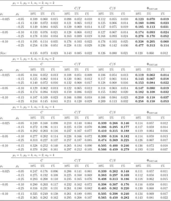
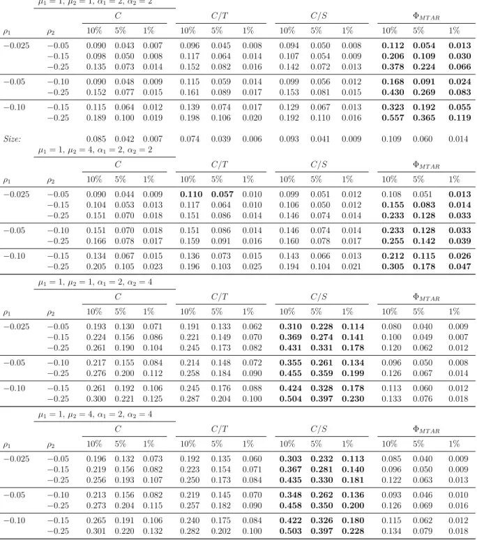
Table 4 reports displays the rejection rates under cointegration with symmetric adjustment and break in either the intercept or slope. The power of the tests is in-vestigated by generating 2,500 draws for every specification. We find that the supF
tests have generally higher rejection rates than either the Engle-Granger test using the ADF test statistic or threshold cointegration tests without breakpoint estimation. The simulation reveals that the supF test with SETAR adjustment has comparable power properties to the GH test. The MTAR specification of the supF test has slightly lower power against the alternative than the GH test. The Enders-Siklos test with SETAR adjustment seems to be rather robust to a break in the intercept but suffers from a drastic reduction in power if a break in the slope is considered. The supF tests appear
to have sufficient power at sample sizes aboveT = 100 and moderate adjustment rate
ρ = −0.5. As expected, the model C outperforms model C/T and C/S if a break in the intercept is considered, whileC/S performs best if the slope changes at one point in the sample.
The simulation results under symmetric adjustment can also be used to analyze the estimation accuracy of the pre-specified breakpoint in the DGP. The timing of the break is varied and takes place either at the beginning, the middle or near the end of the series. The results are summarized inTable 5and reveal that breakpoint estimates are in large parts very accurate. In general, it seems that breaks at the beginning of the sample are most difficult to detect and the supF tests often indicate a later breakpoint. Breaks in the intercept and the slope are estimated with equal accuracy as long as the correct structural break model is applied. The SETAR model seems to produce slightly more accurate breakpoint estimates than the MTAR model.
The upper panel of Table 6 displays the rejection rates under structural stability and asymmetric adjustment. For each combination of autoregressive coefficients, we generate series with sample sizeT = 100. If the series are generated under asymmetric adjustment with a stable cointegrating vector, we find that the supF tests operate with less power than the threshold cointegration tests byEnders and Siklos (2001). Falsely incorporating breaks in form of additional dummy variables in the equilibrium equation thus reduces the power against the null hypothesis. Accordingly, the most parsimonious model C performs best among the three structural break models.
Finally, the behaviour of the supF test is evaluated under parameter instability and asymmetric adjustment. For that matter, we draw from the DGP in (13). We consider SETAR adjustment inTable 6and MTAR adjustment inTable 7, respectively. In the second panel, we model a break in the intercept. The supF tests have poor power properties and are outperformed by the Enders-Siklos test in each parameter combination. The loss in power of the original threshold cointegration test due to a break in the intercept does not justify the additional parameter estimation and grid search of the C model. The C/T and C/S models involve an additional parameter and, as expected, have lower rejection rates. With a break in the slope (third panel of Table 6 and Table 7), we find the picture to be quite different. All structural break models have more power against the null hypothesis than the Enders-Siklos test. As expected, the power of the correctly specified C/S model exceeds all other structural change models for each parameter combination. Further, we evaluate the power of the GH test and find that the power is lower than the supF tests’ power if the adjustment
is asymmetric.5
In the last panel, we display the results for a simultaneous break in the intercept and the slope. Again, theC/S model performs best among the structural break models and far exceeds the benchmark Enders-Siklos test. In general, we find a break in the slope to have a more substantial impact on the power function than a break in the intercept. In practice, we have to assume that structural change involves all parameters of the equilibrium equation. Since the supF tests based on the C/S model perform best in those situations, it has to be considered the preferred model for cointegration relationships with asymmetric adjustment which are subject to parameter instability at an unknown point in time.
5
Empirical application
In this section, we apply the supF test methodology to study the ‘rockets and feathers’ hypothesis6 in the US gasoline market. The ‘rockets and feathers’ hypothesis describes
the adjustment behaviour of prices faced with input price shocks. More precisely, the hypothesis states that prices adjust faster to input price increases than to input price decreases. In the terms ofBacon(1991)’s seminal paper, the price goes up like a rocket, but falls down like a feather. While early studies on the matter (Bacon(1991),Manning
(1991), Borenstein et al. (1997)) focused on the short-run asymmetry in the pricing process, the focus quickly shifted to the economically meaningful long-run asymmetry estimated by asymmetric error correction models (Bachmeier and Griffin (2002)).
For the empirical illustration, we examine the fuel prices transmission at two points of the production chain. First, we analyze the speed of adjustment for deviations from the long-run relationship between crude oil prices and gasoline spot prices (first stage). Second, we analyze the pass-through from gasoline spot prices to retail prices (second stage). Finally, the direct link between crude oil prices and retail prices is analyzed (single stage). Naturally, we expect the speed of adjustment at the first and second stage to be faster than at the single stage transmission. Long-run asymmetry in the sense of the ‘rockets and feathers’ hypothesis is found if negative deviations from the long-run equilibrium are adjusted faster than positive deviations, i.e. ρ1 = ρ− < ρ+ =
ρ2. Alternatively, we use the MTAR model to investigate whether a shock having
5The results are not reported in this paper but can be obtained from the author upon request. 6The name originates from theBacon(1991) paper entitled: ‘Rockets and feathers: the asymmetric
0 100 200 300 400 Retail Spot Crude 2006 2007 2008 2009 2010 2011 2012 2013
Figure 1: WTI crude oil prices, spot gasoline prices and retail gasoline prices from January 2006 to December 2013
momentum greater than or equal to its median is adjusted faster than a shock with less momentum.
Our sample reaches from January 2006 to December 2013 to include the collapse of commodity prices in 2009 and their subsequent recovery. We observe prices at a monthly frequency yielding a total of 96 observations. The West Texas Intermediate prices (pc
t),
regular gasoline spot prices (ps
t) and regular gasoline retail prices (p g
t) are all obtained
from the U.S. Energy Information Administration (EIA).Figure 1depicts the trajectory of the prices and shows volatile behaviour of prices for petroleum products during the Financial Crisis. Although the times series are affected by global events, it does not immediately follow that the long-run relationship between them changes. However, from our simulation study, we know that an existing instability of the cointegrating vector can severely decrease the power of a threshold cointegration test.
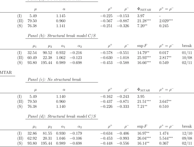
First, we estimate a threshold cointegration model according to Enders and Siklos
(2001). We specify the long-run equilibrium equations (I) ps t = µ+α pct+et (II) pgt = µ+α ps t +et (S) pgt = µ+α pc t+et (14)
coefficients of the cointegrating vector are estimated using least squares and a threshold model is applied to the residuals. The results for the SETAR model are reported in panel (a) ofTable 8 and reveal significant asymmetry in the adjustment process only in the second stage. The results for the MTAR model with u= 0.5 are reported in panel (b) ofTable 8. Here, we also find significant asymmetries in the transmission from spot gasoline to retail gasoline prices. Surprisingly, we do not find sufficient evidence for a long-run relationship between crude oil prices and gasoline spot prices. In contrast, retail gasoline prices and crude oil prices seem to maintain a long-run equilibrium which is a less likely result from an economic perspective than the existence of a crude/spot relationship.
Second, we estimate the long-run equilibrium equations again using theC/S specifi-cation since this specifispecifi-cation of the supF tests performed best in the simulation study if the slope coefficient changed at one point in time and is best-suited for modelling unspecific regime shift events. The results are reported in panel (b) and panel (d) of
Table 8. The null hypothesis of no cointegration can now be rejected at all stages along the gasoline value-chain. The breakpoint is located either at the peak crude oil prices during the Financial Crisis or after the prices had recovered in 2011. Closer inspection of the time series reveals that the spread between crude oil prices and spot gasoline prices increased substantially around 2011. We do not find statistical evidence for asymmetric adjustment processes in the first stage. The asymmetry results for the second stage and single stage remain unchanged.
6
Summary
This paper proposed an extension to the GH test to include SETAR and MTAR ad-justment. Thereby, we constructed threshold cointegration tests which endogenously determine the location of a structural break in the cointegrating vector and test the null of no cointegration. We derived the limiting distribution for the structural break models C, C/T and C/S and tabulated their critical values which were obtained by Monte Carlo simulations. Analysis of the finite sample properties under the alterna-tive of linear and threshold cointegration revealed that the tests exhibit considerable power gains over the conventional Enders-Siklos tests if a break in the slope coefficient is present. We applied the supF tests to US gasoline market data and found evidence for a long-run relationship between prices along the value-chain after we accounted for
structural breaks. The results for the SETAR and MTAR models provided evidence for asymmetric price transmission from spot gasoline to retail gasoline.
7
Acknowledgement
I thank Karl-Heinz Schild, Karlheinz Fleischer, Robert Jung, Martin Wagner and Kon-stantin Kuck for valuable comments and suggestions. Further, I thank seminar partic-ipants at the University of Marburg, University of Hohenheim, University of Tübingen and Technical University Dortmund, as well as participants of the THE Christmas Workshop in Stuttgart and the German Statistical Week in Rostock. Access to Thom-son Reuters Datastream, provided by the Hohenheim Datalab (DALAHO), is gratefully acknowledged.
Appendix
Proof of Theorem 1. The asymptotic distribution is derived by adapting the results of Gregory and Hansen (1992) to match the F-statistic process involving a threshold indicator function using results in Maki and Kitasaka (2015). However, Maki and Kitasaka (2015) use a different definition of the threshold parameter space in their SETAR model. The threshold parameter in our model is fixed, i.e. belongs to a trivial compact subset of R whereas the parameter space in Maki and Kitasaka (2015) is data dependent (see the discussion on threshold parameter space in Section 2.2 of their paper). Indicator functions with threshold parameters defined on compact sets are treated in Seo (2008). The proof only refers to model C/S while the results for the remaining models can be deduced from the results obtained for this model. Hence, we consider the cointegrating regression,
yt = ˆα01xt+ ˆµ1+ ˆα20xtϕt,τ + ˆµ2ϕt,τ + ˆetτ, (15)
where ˆetτ is an integrated process under the null hypothesis of no cointegration and
zt= (yt, x0t)0 is generated according to (6).
Define the (2m + 3)-vector Xtτ = (yt, xt0,1, xtϕt,τ0, ϕt,τ)0 and partition Xtτ =
(X1tτ, X2tτ0)0 where X1tτ = yt and X2tτ contains all regressors of (15).
De-fine δT = diag(T−1/2Im+1,1, T−1/2Im,1), ϕτ(s) = 1{s > τ} and Xτ(s) =
(B(s)0,1, Bx(s)ϕτ(s)
0
, ϕτ(s))0. PartitionδT = (δ1T, δ2T) in conformity toXtτ.
Next, we partition the (m + 1)-vector standard Brownian Motion W as W = (Wy, Wx0) 0 where Wy = l−111 By−ω210 Ω −1 22Bx Wx = Ω −1/2 22 Bx. (16) Furthermore, we define Wxτ = (Wx0,1, Wxϕτ0, ϕτ)0 (17) and Wτ = (Wy, Wxτ0)0.
First, we consider the least squares estimator of the parameters of the cointegrating regression. It is shown in Gregory and Hansen (1992) using the FCLT for vector pro-cesses inPhillips and Durlauf (1986) and the continuous mapping theorem (CMT, see
Billingsley (1999), Theorem 2.7) that T−1δT T X t=1 XtτXtτ0δT ⇒ 1 Z 0 XτXτ0 (18)
where the weak convergence is with respect to the uniform metric over τ ∈ T. In the remainder of the proof, we refer to weak convergence results involving the break fraction parameter τ as holding uniformly over τ (see also Arai and Kurozumi (2007) for a similar application).
We define the vector ˆθτ = ( ˆα01,µˆ1,αˆ02,µˆ2) as the least squares estimator of (15) for eachτ. It follows from (18) and the CMT that
T−1/2δ2−T1θˆτ = T−1δ2T T X t=1 X2tτX2tτ0δ2T !−1 T−1δ2T T X t=1 X2tτX1tτδ1T ! ⇒ 1 Z 0 X2τX2τ0 −1 1 Z 0 X2τX1τ . (19) When we set ˆητ =T−1/2δT−1(1,−θˆ 0 τ) 0 = (1,−δ−1 2Tθˆ 0 τ) 0, it follows that ˆ ητ ⇒ 1,− 1 Z 0 X1τX2τ0 1 Z 0 X2τX2τ0 −1 0 =ητ. (20)
Next, we state some useful convergence results for the residuals of the cointegrating regression. We define the residual series ˆetτ =yt−αˆ01xt−µˆ1−αˆ02xtϕt,τ−µˆ2ϕt,τ which
is dependent onτ. Note that ˆetτ can be expressed as
ˆ
etτ =T1/2ηˆτ0δTXtτ. (21)
Using Lemma 2.2 of Phillips and Ouliaris (1990) yields
where κτ = 1,− 1 Z 0 WyWxτ0 1 Z 0 WxτWxτ0 −1 0 Lητ = l11κτ (23) Qκτ = Wy− 1 Z 0 WyWxτ0 1 Z 0 WxτWxτ0 −1 Wxτ.
The first-differenced residuals are expressed as ∆ˆetτ =T1/2ηˆτ0δT∆Xtτ, where
∆Xtτ = ∆(yt, xt0,1, xtϕt,τ0, ϕt,τ)0 = (ξ1t, ξ2t0,0, xt−1∆ϕt,τ0+ ∆xtϕt,τ0,∆ϕt,τ)0 (24) = (ξ1t, ξ2t0,0, xt−1∆ϕt,τ +ξ2tϕt,τ0,∆ϕt,τ)0 and ∆ϕt,τ = 1 if t= [T τ] 0 if t6= [T τ] . (25)
The asymptotic counterpart to ∆ϕt,τ is the differential dϕτ, a Dirac function
concen-trating the unit mass at the pointt=τ so that
b
Z
a
f dϕτ = lim
z↑τ f(z), a < τ < b,
for all functions with left-limits. Then, we can define the differentialdXτ by
dXτ(s) = (dB(s)0,0, Bx(s)0dϕτ(s) +dBx(s)0ϕτ(s), dϕτ(s))0. (26)
Under Assumption (1),ξt is a stationary VARMA process and consequently, the scalar
process T1/2ηˆ0
τδT∆Xtτ ⇒ T1/2ητ0δT∆Xtτ is also a stationary ARMA process with an
intervention outlier at t = [T τ]. Moreover, under Assumption (3) the lag truncation parameter K → ∞ for T → ∞. This means that the error of approximating tτ by
a finite AR process becomes small as K grows large. Following Phillips and Ouliaris
(1990) we write the infinite order AR representation of the SETAR error term process as
tτ =
∞
P
j=0
Dj(T1/2δT∆Xt−jτ)0ητ =D(L)(T1/2δT∆Xtτ)0ητ. The lag structure is chosen in
D(1)2η0
τΩτητ. From Lemma 2.1 of Phillips and Ouliaris (1990), it follows that
T−1/2 [T s] X t=1 tτ K =D(L)η0τ T −1/2 [T s] X t=1 T1/2δT∆Xtτ +op(1) ⇒D(1)η 0 τXτ(s), (27) whereD(1) = P∞ j=0 Dj.
Now, we consider the auxiliary regression. We apply the SETAR model to the residuals according to (4) and compute the test statistics Fτ. Note that the
esti-mated adjustment coefficients might be correlated with the estiesti-mated coefficients of the additional lagged differences. Therefore, we write the least squares estimator of
ρ= (ρ1, ρ2)0 in the breakpoint specific notation under the null hypothesis ρ1 =ρ2 = 0 as ˆρ= (Uτ0QKUτ)−1Uτ0QKτ, where Uτ = ˆ e0τ1{eˆ0τ ≥λ} eˆ0τ1{eˆ0τ < λ} ˆ e1τ1{eˆ1τ ≥λ} eˆ1τ1{eˆ1τ < λ} .. . ... ˆ eT−1τ1{eˆT−1τ ≥λ} eˆT−1τ1{eˆT−1τ < λ} , (28)
τ = (1τ, 2τ, . . . , T τ)0 and QK =I−MK(MK0 MK)−1MK0 is the projection matrix onto
the space orthogonal to the regressors MK = (∆ˆet−1τ, . . . ,∆ˆet−Kτ).
Partition the matrix Uτ asUτ = (U1τ, U2τ), then the t ratio of ˆρ1 can be expressed as t1 = ˆ ρ1 se(ˆρ1) = ρˆ1 (ˆσ2(U0 1τQKU1τ)−1)1/2 = U 0 1τQKτ ˆ σ(U10τQKU1τ)1/2 (29) and similarly the t ratio of ˆρ2 can be expressed as
t2 =
U20τQKτ
ˆ
σ(U20τQKU2τ)1/2
. (30)
In the remainder of the proof, we focus on t1. Scaling the t ratio appropriately yields the numerator
T−1U10τQKτ = T−1U10ττ −T−1/2·T−1U10τMK(T−1MK0 MK)−1T−1/2MK0 τ
and the term
T−2U10τQKU1τ = T−2U10τU1τ −T−1·T−1U10τMK(T−1MK0 MK)−1T−1MK0 U1τ
= T−2U10τU1τ +op(1) =DT(λ, τ) +op(1). (32)
Finally, we need convergence results for NT(λ, τ), DT(λ, τ) and ˆσ2. Since x 7→
x1{x≥λ} is a regular function, it follows from (22) and Theorem 3.1 of Park and Phillips(2001) that
T−1/2eˆt−1τ1{eˆt−1τ ≥λ} = ηˆτ0δTXt−1τ1{T1/2ηˆ0τδTXt−1τ ≥λ}
= ηˆτ0δTXt−1τ1{ηˆτ0δTXt−1τ ≥T−1/2λ} (33)
⇒ ητ0Xτ1{η0τXτ ≥0}=l11Qκτ1{Qκτ ≥0}.
Thus, Theorem 2.2 of Kurtz and Protter (1991) combined with results (27) and (33) yields NT(λ, τ) = T−1 T X t=1 1{ˆet−1τ ≥λ}ˆet−1τtτ = ηˆτ0δT T X t=1 1{δTηˆ0τXt−1τ ≥T−1/2λ}Xt−1τD(L)(∆Xtτ)0δTητ ⇒ D(1)ητ0 1 Z 0 1{ητ0Xτ ≥0}XτdXτ0ητ (34) = D(1)l211 1 Z 0 1{Qκτ ≥0}QκτdQκτ,
while (27), (33) and the CMT yield
DT(λ, τ) = T−2 T X t=1 1{ˆet−1τ ≥λ}eˆ2t−1τ = ηˆτ0δTT−1 T X t=1 1{δTηˆτ0Xt−1τ ≥T−1/2λ}Xt−1τXt−1τ0δTηˆτ ⇒ ητ0 1 Z 0 1{ητ0Xτ ≥0}XτXτ0ητ (35) = l211 1 Z 0 1{Qκτ ≥0}Q2κτ.
For the variance estimate, ˆσ2, we note that ˆρ
1 = Op(T−1) and ˆρ2 = Op(T−1), but
(ˆγj −γj) =Op(T−1/2). Using Lemma 2.2 of Phillips and Ouliaris (1990) yields
ˆ σ2 = T−1 T X t=1 ∆ˆetτ −ρˆ1eˆt−1τ1{eˆt−1τ ≥λ} −ρˆ2eˆt−1τ1{ˆet−1τ < λ} − K X j=1 ˆ γj∆ˆet−jτ 2 = T−1 T X t=1 2tτ +op(1) ⇒D(1)2ητ0Ωτητ =D(1)2l211κ 0 τDτκτ, (36)
where the long-run covariance matrix is given by
Ωτ = ω11 ω210 0 (1−τ)ω 0 21 0 ω21 Ω22 0 (1−τ)Ω22 0 0 0 0 0 0 (1−τ)ω21 (1−τ)Ω22 0 (1−τ)Ω22 0 0 0 0 0 0 (37) and Dτ = 1 0 0 0 0 0 Im 0 (1−τ)Im 0 0 0 0 0 0 0 (1−τ)Im 0 (1−τ)Im 0 0 0 0 0 0 . (38)
Similar results can be obtained for t2 so that the results (34), (35), (36) combine with the CMT to proof the theorem under the null hypothesis.
Under the alternative, the system is cointegrated so that we have ˆητ p
→ητ and
ˆ
ητ =ητ+Op(T−1) (39)
from Phillips and Durlauf (1986), Theorem 4.1. Thus, for the residual series it holds that
ˆ
etτ = ˆητ0zt=η0τzt+Op(T−1/2) = qtητ +Op(T−1/2). (40)
By assumption a stationary SETAR representation of qtητ exists and is given by
qtητ =a11qt−1ητ1{qt−1ητ ≥λ}+a12qt−1ητ1{qt−1ητ < λ}+
∞
X
j=2
where∗tητ is an orthogonal (0, σ∗
ητ) sequence. This can alternatively be written as
∆qtητ =ψ11qt−1ητ1{qt−1ητ ≥λ}+ψ12qt−1ητ1{qt−1ητ < λ}+
∞
X
j=2
ψj∆qt−jητ +∗tητ. (42)
If we consider the t ratio of ˆρ1 and use the expression
t1 = 1 ˆ σ ˆ ρ1(U10τQKU1τ)1/2 , (43) we find that ˆρ1 p →ψ116= 0 and ˆσ2 p →σ2 ∗ ητ. Further, we observe U10τQKU1τ =U10τU1τ −U10τMK(MK0 MK)−1MK0 U1τ =Op(T) (44)
which yields t1 = Op(T1/2) and similarly t2 = Op(T1/2). Hence, we immediately see
that FSET AR∗ → ∞ as T → ∞.
Proof of Theorem 2. The proof is structured similarly to the proof of Theorem 1. Using the results for the cointegrating regression, we write the AR representation of the MTAR error term process astτ =
∞
P
j=0
aj(T−1/2δT∆Xt−jτ)0ητ =a(L)(T−1/2δT∆Xt−jτ)0ητ
and tτ is an orthogonal (0, σ2(η, τ)) sequence with σ2(η, τ) = a(1)2η0τΩτητ. From
Lemma 2.1 of Phillips and Ouliaris (1990), it follows that
T−1/2 [T s] X t=1 tτ K =a(L)ητ0 T −1/2 [T s] X t=1 T1/2δT∆Xtτ +op(1)⇒a(1)ητ0Xτ, (45) wherea(1) = P∞ j=0 aj.
Now, we apply the MTAR model to the residuals according to (5) and compute the test statisticsFτ. The t ratio of ˆρ1 is written as
t1 =
U10τQKτ
ˆ
σ(U10τQKU1τ)1/2
(46)
and thet ratio of ˆρ2 is written as
t2 =
U20τQKτ
ˆ
σ(U20τQKU2τ)1/2
where Uτ = (U1τ, U2τ) = ˆ e0τ1{∆ˆe0τ ≥λ} eˆ0τ1{∆ˆe0τ < λ} ˆ e1τ1{∆ˆe1τ ≥λ} eˆ1τ1{∆ˆe1τ < λ} .. . ... ˆ eT−1τ1{∆ˆeT−1τ ≥λ} eˆT−1τ1{∆ˆeT−1τ < λ} . (48)
Finally, we need convergence results for NT(λ, τ), DT(λ, τ) and ˆσ2. The main
dif-ference between the asymptotic distribution for the SETAR and the MTAR models lies in the fact that the indicator variable ∆ˆetτ has a stationary distribution under the
null hypothesis and the alternative. Further, the MTAR decomposition of ˆet−1τ is not
regular and Theorem 3.1 of Park and Phillips (2001) cannot be used. However, from Theorem 1 in Caner and Hansen (2001) it follows that
T−1/2 [T s] X t=1 1{∆ˆet−1τ ≥λ}tτ = T−1/2 [T s] X t=1 1{G(∆ˆet−1τ)≥G(λ)}tτ = T−1/2 [T s] X t=1 1{Ut≥G(λ)}tτ ⇒ Qκτ(s, u) = σ(η, τ)W(s, u) (49) = a(1)l11(κ0τDτκτ)1/2W(s, u),
where G(·) is the marginal distribution of ∆ˆet−1τ so that G(∆ˆet−1τ) = Ut ∼ U[0,1]
and G(λ) = u. The standard two-parameter Brownian motion W(s, u) is defined on (s, u)∈[0,1]2. Using Theorem 2.2 ofKurtz and Protter (1991) and (49) yields
NT(λ, τ) = T−1 T X t=1 1{∆ˆet−1τ ≥λ}eˆt−1τtτ = ηˆ0τδT T X t=1 1{G(∆ˆet−1τ)≥G(λ)}Xt−1τtτ ⇒ a(1)l11(κ0τDτκτ)1/2ητ0 1 Z 0 Xτ(s)dW(s, u) (50) = a(1)l211(κτ0Dτκτ)1/2 1 Z 0 Qκτ(s)dW(s, u)
and Theorem 3 ofCaner and Hansen (2001) yields DT(λ, τ) = T−2 T X t=1 1{∆ˆet−1τ ≥λ}ˆe2t−1τ = ηˆτ0δTT−1 T X t=1 1{G(∆ˆet−1τ)≥G(λ)}Xt−1τXt−1τ0δTηˆτ ⇒ uητ0 1 Z 0 Xτ(s)Xτ0(s)dsητ (51) = ul112 1 Z 0 Q2κτ(s)ds.
For the variance estimate, ˆσ2, Lemma 2.2 of Phillips and Ouliaris (1990) yields
ˆ σ2 = T−1 T X t=1 2tτ +op(1) ⇒ a(1)2l211κ0τDτκτ. (52)
The results (50), (51), (52) combine with the CMT to proof
t1 ⇒ 1 R 0 Qκτ(s)dW(s, u) u 1 R 0 Q2 κτ(s)ds !1/2. (53)
Analogously, we can show that
t2 ⇒ 1 R 0 Qκτ(s) (dW(s,1)−dW(s, u)) (1−u) 1 R 0 Q2 κτ(s)ds !1/2 (54)
holds. Finally, we observe that taking the supremum over all τ ∈ T is a continuous transformation so that we can use the CMT to proof the theorem under the null hypoth-esis. The proof of the theorem under the alternative is a straightforward adaptation of
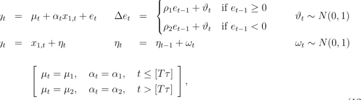
Table 1: Approximate critical values of FSET AR∗ C C/T C/S T 90% 95% 99% 90% 95% 99% 90% 95% 99% m= 1 50 16.01 18.48 24.22 18.80 21.38 27.10 17.52 20.16 25.83 100 12.73 14.66 19.24 15.58 17.75 22.49 14.44 16.68 21.40 250 10.80 12.29 15.70 12.99 14.59 18.16 12.52 14.36 17.82 500 10.13 11.42 14.30 12.11 13.46 16.37 11.76 13.24 16.39 ∞ 9.48 10.70 13.45 11.53 12.86 15.74 11.20 12.71 15.69 m= 2 50 17.63 20.14 26.26 19.84 22.42 28.47 20.49 23.47 29.57 100 16.19 18.21 23.21 18.69 20.90 25.94 19.24 21.56 26.54 250 13.33 15.02 18.93 15.50 17.39 21.69 16.47 18.39 23.03 500 12.22 13.68 17.08 14.06 15.63 19.07 15.22 16.85 20.18 ∞ 12.18 13.60 16.88 14.22 15.82 19.33 15.30 16.86 20.45 m= 3 50 19.80 22.49 28.40 21.71 24.56 30.57 23.94 27.05 34.08 100 18.20 20.51 25.37 20.40 22.81 28.00 22.87 25.43 30.89 250 15.37 17.16 21.21 17.31 19.24 23.42 19.81 22.00 26.48 500 14.15 15.71 19.11 15.88 17.57 21.14 18.44 20.30 24.11 ∞ 14.12 15.65 19.03 16.00 17.66 21.23 18.60 20.44 24.09 m= 4 50 21.19 23.92 29.90 23.22 26.11 32.96 27.33 30.40 37.89 100 20.13 22.56 27.61 22.42 24.80 29.47 25.98 28.49 34.16 250 17.36 19.27 23.87 19.21 21.23 26.12 23.26 25.81 30.78 500 15.77 17.41 20.70 17.41 19.13 22.73 21.46 23.44 27.80 ∞ 16.04 17.69 21.28 17.81 19.51 23.12 21.75 23.83 27.95
Note: C,C/T andC/S denote the supF tests using the structural break models in (3). m refers to the number of columns of the regressor matrixxt. The lag truncation parameter is determined using
the BIC and maximum lag lengthKmax= 8. Critical values for different order selection rules are not
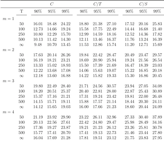
Table 2: Approximate critical values ofFM T AR∗ C C/T C/S u 90% 95% 99% 90% 95% 99% 90% 95% 99% m= 1 T= 50 0.15 17.49 20.18 26.82 18.72 21.25 26.65 18.12 20.62 26.60 0.25 16.89 19.41 25.74 18.56 20.86 26.52 17.98 20.43 26.32 0.50 16.56 19.03 24.57 18.51 20.94 26.52 17.88 20.34 26.00 T = 100 0.15 17.95 21.03 28.71 18.16 20.77 26.43 18.04 21.17 28.37 0.25 15.56 18.26 24.05 17.03 19.32 24.00 16.55 18.97 24.92 0.50 14.58 16.86 21.30 16.47 18.92 23.86 15.92 18.28 23.42 T = 250 0.15 19.21 23.19 32.09 18.82 21.85 28.79 19.45 23.15 31.94 0.25 15.08 17.60 24.11 16.11 18.20 23.65 16.13 18.65 25.27 0.50 12.85 14.72 18.87 14.75 16.50 20.70 14.33 16.21 20.98 T = 500 0.15 20.83 24.76 35.04 20.90 24.37 32.96 21.56 25.51 35.91 0.25 15.35 17.67 24.79 16.60 18.98 24.46 16.55 18.95 25.93 0.50 12.49 14.04 17.37 14.34 15.89 19.51 13.96 15.66 19.37 T=∞ 0.15 21.59 25.94 36.86 21.52 25.25 34.64 22.52 26.71 37.94 0.25 15.30 17.48 25.12 16.37 18.67 24.70 16.56 19.01 26.38 0.50 11.81 13.13 16.39 13.65 14.82 18.08 13.35 14.79 18.27 m= 2 T= 50 0.15 18.18 20.74 26.68 19.72 22.13 28.33 20.23 22.86 29.18 0.25 17.95 20.36 26.17 19.64 21.99 27.80 20.37 23.05 29.61 0.50 17.77 20.24 26.40 19.91 22.40 28.33 20.44 23.38 29.22 T = 100 0.15 18.74 21.57 27.97 19.57 22.19 28.05 20.01 22.43 28.48 0.25 17.21 19.08 25.53 18.84 21.23 26.08 19.62 21.93 27.02 0.50 16.84 19.15 24.07 18.84 21.09 25.82 19.62 21.13 27.15 T = 250 0.15 19.85 23.35 32.90 19.81 22.51 28.71 20.89 23.90 31.19 0.25 16.43 18.77 24.80 17.53 19.73 24.53 18.64 21.00 26.47 0.50 14.70 16.64 20.91 16.48 18.35 22.44 17.46 19.56 24.40 T = 500 0.15 21.24 25.01 35.89 21.49 24.69 31.92 22.52 26.01 35.26 0.25 16.54 18.96 26.23 17.70 19.77 24.76 18.62 21.19 27.14 0.50 14.26 15.90 19.66 15.86 17.51 21.06 16.97 18.75 23.10 T=∞ 0.15 21.88 26.00 38.63 21.79 25.05 32.61 23.17 27.05 37.19 0.25 16.23 18.99 26.06 17.12 19.07 24.19 18.20 20.87 27.27 0.50 13.20 14.64 18.18 14.69 16.14 19.47 15.88 17.47 21.79
Note: C,C/T andC/Sdenote the structural break models in (3). mrefers to the number of columns of the regressor matrixxt. The lag truncation parameter is determined using the BIC and maximum
lag lengthKmax = 8. Critical values for different order selection rules are not reported but can be
obtained from the author upon request. Critical values foru={0.75,0.85}are not reported to conserve space. Since the distribution is symmetric inu, the values can easily be inferred from the table.
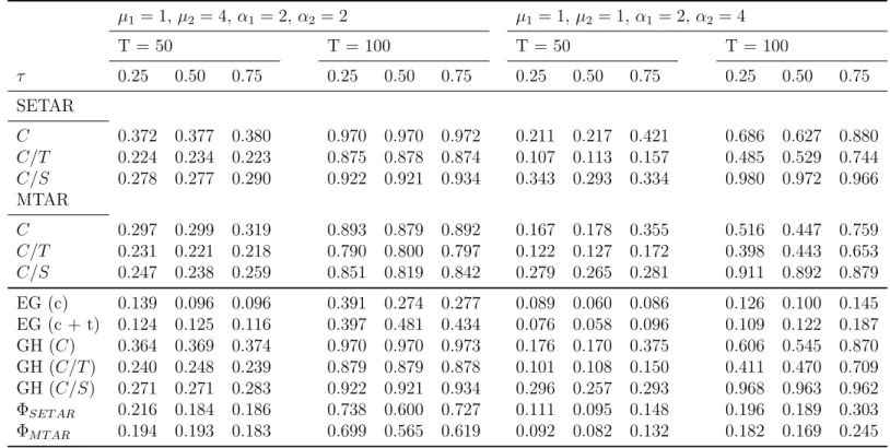
Table 3: Approximate critical values of FM T AR∗ , continued C C/T C/S u 90% 95% 99% 90% 95% 99% 90% 95% 99% m= 3 T= 50 0.15 19.72 22.32 27.81 21.40 24.06 30.13 23.59 26.77 33.19 0.25 19.73 22.47 27.92 21.55 24.10 29.93 23.72 26.87 33.77 0.50 19.86 22.37 28.41 21.60 24.49 30.78 24.13 27.36 34.55 T = 100 0.15 19.74 22.37 28.26 21.05 23.53 28.71 22.89 25.54 30.77 0.25 18.90 21.17 26.30 20.50 22.95 27.94 22.77 25.36 30.68 0.50 18.66 21.03 25.79 20.51 22.89 28.32 22.90 25.71 31.06 T = 250 0.15 20.12 23.50 31.76 20.66 23.36 28.98 22.49 25.25 31.63 0.25 17.66 20.05 26.40 18.94 21.00 25.55 21.07 23.50 29.01 0.50 16.52 18.40 22.78 18.17 20.05 24.18 20.52 22.73 27.76 T = 500 0.15 21.79 25.58 34.78 22.22 25.74 33.58 23.45 26.54 34.99 0.25 17.92 20.37 26.21 19.01 21.17 27.07 20.88 23.27 28.54 0.50 15.94 17.76 21.83 17.45 19.21 23.49 19.77 21.75 26.03 T=∞ 0.15 22.14 26.37 36.87 22.20 25.94 34.35 23.42 26.67 36.10 0.25 17.39 19.98 26.48 18.33 20.30 26.20 20.08 22.46 28.03 0.50 14.91 16.48 20.49 16.28 17.83 21.55 18.60 20.29 24.59 m= 4 T= 50 0.15 21.12 23.88 29.68 22.90 25.88 31.96 26.96 30.13 36.84 0.25 21.08 23.84 29.93 23.04 25.89 31.99 27.21 30.20 37.04 0.50 21.33 24.07 30.30 23.29 26.13 32.80 27.65 30.68 37.73 T = 100 0.15 21.05 23.51 29.54 22.43 24.71 30.01 25.57 28.29 33.88 0.25 20.52 22.93 27.47 22.31 24.65 29.63 25.77 28.31 34.02 0.50 20.49 22.93 27.85 22.43 24.91 30.01 26.15 28.71 34.65 T = 250 0.15 21.03 23.88 31.30 21.75 24.39 29.32 24.56 27.12 32.56 0.25 19.15 21.26 26.57 20.50 22.62 27.36 23.84 26.21 31.76 0.50 18.24 20.24 24.79 19.83 21.87 26.58 23.61 26.01 31.68 T = 500 0.15 22.38 25.85 35.15 22.59 25.57 33.44 25.12 28.03 35.57 0.25 18.89 21.28 27.64 19.98 22.11 27.03 23.28 25.52 30.62 0.50 17.43 19.27 23.32 18.82 20.71 24.71 22.37 24.53 29.27 T=∞ 0.15 22.50 26.28 36.47 22.37 25.67 33.72 24.82 27.74 35.55 0.25 18.21 20.51 27.60 19.06 21.15 26.11 22.39 24.59 29.73 0.50 16.26 17.90 21.89 17.45 19.14 23.09 21.10 23.22 27.89
Table 4: Size-adjusted power of the supF test under structural change and symmetric adjustment µ1= 1,µ2= 4, α1= 2,α2= 2 µ1= 1,µ2= 1,α1= 2,α2= 4 T = 50 T = 100 T = 50 T = 100 τ 0.25 0.50 0.75 0.25 0.50 0.75 0.25 0.50 0.75 0.25 0.50 0.75 SETAR C 0.372 0.377 0.380 0.970 0.970 0.972 0.211 0.217 0.421 0.686 0.627 0.880 C/T 0.224 0.234 0.223 0.875 0.878 0.874 0.107 0.113 0.157 0.485 0.529 0.744 C/S 0.278 0.277 0.290 0.922 0.921 0.934 0.343 0.293 0.334 0.980 0.972 0.966 MTAR C 0.297 0.299 0.319 0.893 0.879 0.892 0.167 0.178 0.355 0.516 0.447 0.759 C/T 0.231 0.221 0.218 0.790 0.800 0.797 0.122 0.127 0.172 0.398 0.443 0.653 C/S 0.247 0.238 0.259 0.851 0.819 0.842 0.279 0.265 0.281 0.911 0.892 0.879 EG (c) 0.139 0.096 0.096 0.391 0.274 0.277 0.089 0.060 0.086 0.126 0.100 0.145 EG (c + t) 0.124 0.125 0.116 0.397 0.481 0.434 0.076 0.058 0.096 0.109 0.122 0.187 GH (C) 0.364 0.369 0.374 0.970 0.970 0.973 0.176 0.170 0.375 0.606 0.545 0.870 GH (C/T) 0.240 0.248 0.239 0.879 0.879 0.878 0.101 0.108 0.150 0.411 0.470 0.709 GH (C/S) 0.271 0.271 0.283 0.922 0.921 0.934 0.296 0.257 0.293 0.968 0.963 0.962 ΦSET AR 0.216 0.184 0.186 0.738 0.600 0.727 0.111 0.095 0.148 0.196 0.189 0.303 ΦM T AR 0.194 0.193 0.183 0.699 0.565 0.619 0.092 0.082 0.132 0.182 0.169 0.245
Note: C,C/T andC/S denote the structural break models in (3). EG (c) and EG (c + t) refer to the Engle-Granger test with intercept and intercept plus trend, respectively. GH denotes the Gregory-Hansen test. ΦSET ARand ΦM T ARdenote the Enders-Siklos cointegration test with SETAR and MTAR adjustment, respectively.
The table is based on 2,500 replications of the DGP described in (13). The autoregressive coefficients areρ1=ρ2=−0.5, i.e. the adjustment is constant and symmetric.
Table 5: Estimates of the breakpoint under symmetric adjustment SETAR µ1= 1,µ2= 4,α1= 2,α2= 2 µ1= 1,µ2= 1,α1= 2,α2= 4 T = 50 T = 100 T = 50 T = 100 τ 0.25 0.50 0.75 0.25 0.50 0.75 0.25 0.50 0.75 0.25 0.50 0.75 C 0.32(0.15) 0.53(0.11) 0.70(0.15) 0.28(0.10) 0.51(0.08) 0.74(0.11) 0.34(0.18) 0.55(0.13) 0.72(0.13) 0.28(0.12) 0.54(0.11) 0.75(0.10) 0.28(0.04) 0.52(0.04) 0.74(0.04) 0.26(0.02) 0.51(0.02) 0.76(0.02) 0.28(0.05) 0.54(0.04) 0.76(0.04) 0.26(0.02) 0.52(0.02) 0.77(0.02) C/T 0.38(0.19) 0.50(0.16) 0.66(0.22) 0.33(0.16) 0.51(0.11) 0.69(0.16) 0.39(0.19) 0.53(0.15) 0.65(0.20) 0.31(0.15) 0.53(0.11) 0.73(0.13) 0.28(0.26) 0.50(0.08) 0.74(0.34) 0.27(0.03) 0.51(0.02) 0.75(0.03) 0.28(0.26) 0.52(0.10) 0.74(0.22) 0.27(0.02) 0.52(0.02) 0.75(0.02) C/S 0.35(0.16) 0.53(0.12) 0.68(0.16) 0.30(0.11) 0.51(0.07) 0.72(0.12) 0.33(0.14) 0.54(0.09) 0.71(0.13) 0.27(0.07) 0.51(0.05) 0.75(0.07) 0.28(0.18) 0.54(0.04) 0.76(0.12) 0.25(0.02) 0.51(0.02) 0.76(0.03) 0.26(0.14) 0.54(0.04) 0.78(0.08) 0.25(0.02) 0.51(0.02) 0.77(0.01) MTAR µ1= 1,µ2= 4,α1= 2,α2= 2 µ1= 1,µ2= 1,α1= 2,α2= 4 T = 50 T = 100 T = 50 T = 100 τ 0.25 0.50 0.75 0.25 0.50 0.75 0.25 0.50 0.75 0.25 0.50 0.75 C 0.35(0.18) 0.52(0.14) 0.68(0.18) 0.29(0.11) 0.51(0.08) 0.74(0.10) 0.38(0.22) 0.55(0.21) 0.67(0.21) 0.30(0.17) 0.54(0.17) 0.72(0.17) 0.28(0.14) 0.52(0.04) 0.74(0.10) 0.26(0.02) 0.51(0.02) 0.75(0.02) 0.28(0.30) 0.54(0.20) 0.74(0.04) 0.27(0.02) 0.52(0.09) 0.77(0.02) C/T 0.40(0.20) 0.50(0.16) 0.60(0.22) 0.34(0.17) 0.51(0.12) 0.68(0.17) 0.42(0.21) 0.53(0.18) 0.64(0.21) 0.35(0.18) 0.54(0.15) 0.72(0.15) 0.28(0.34) 0.50(0.08) 0.72(0.38) 0.27(0.04) 0.51(0.02) 0.75(0.05) 0.32(0.32) 0.54(0.14) 0.74(0.26) 0.27(0.13) 0.52(0.07) 0.76(0.02) C/S 0.38(0.18) 0.53(0.14) 0.67(0.17) 0.31(0.12) 0.51(0.08) 0.72(0.11) 0.36(0.17) 0.52(0.16) 0.66(0.22) 0.27(0.09) 0.50(0.10) 0.72(0.16) 0.30(0.26) 0.52(0.06) 0.74(0.18) 0.26(0.04) 0.52(0.02) 0.76(0.03) 0.30(0.22) 0.54(0.06) 0.76(0.16) 0.25(0.02) 0.52(0.02) 0.77(0.02)
Note: C,C/T andC/Sdenote the structural break models in (3). The left panel and right panel report the estimates of the break fraction following a shift in the intercept and a shift in the slope, respectively. Upper rows contain the mean breakpoint estimate and the empirical standard deviation. Lower row contain the median breakpoint and the interquartile range. The autoregressive coefficients areρ1=ρ2=−0.5, i.e. the adjustment is constant and symmetric.