A Monad for Randomized Algorithms
Tyler Barker
1Mathematics Tulane University New Orleans, LA, USA
Abstract
In this paper, we introduce a monad of random choice for domains that does not suffer from the main two drawbacks of the probabilistic powerdomain. It is not known whether any Cartesian closed category of domains is closed under the probabilistic powerdomain, but the Cartesian closed category BCDis closed under this monad of random choice. Also, there is no distributive law between the probabilistic powerdomain and any of the nondeterministic powerdomains, but there is a distributive law between the monad of random choice and the lower powerdomain. In order to work with the convex powerdomain, an alteration to the monad of random choice is made, so that the Cartesian closed categoriesRBandFSare closed under this construction. Then, in these categories, there is a distributive law between this monad and the convex powerdomain. This work is based on the uniform continuous random variables of Goubault-Larrecq and Varacca, which do not form a monad. This paper gives motivation for this model and changes the definition of the Kleisli extension of Goubault-Larrecq and Varacca so that it is monotone, which was the problem with their definition.
Keywords: Probabilistic powerdomain, Cartesian closed category, random variable, distributive law
1
Introduction
Starting with Dana Scott’s model of the untyped lambda calculus, domain theory has been largely successful in providing models of computation. The use of domain theory has expanded to provide denotational semantics for many computational effects, such as continuations and nondeterminism, using Moggi’s [16] monadic ap-proach. One type of computation that has been problematic to model, however, is probabilistic computation. The most well known monad of probabilistic computa-tion is the probabilistic powerdomain, first defined by Saheb-Djahromi in 1980 [18]. However, this monad has two major flaws [11]. First, there is no distributive law between the probabilistic powerdomain and any of the three nondeterministic pow-erdomains [24]. According to Beck’s Theorem [4], the composition of two monads is a monad if and only if the monads satisfy a distributive law. Thus, to generate
1 Email:[email protected]
Electronic Notes in Theoretical Computer Science 325 (2016) 47–62
1571-0661/© 2016 The Author(s). Published by Elsevier B.V.
www.elsevier.com/locate/entcs
http://dx.doi.org/10.1016/j.entcs.2016.09.031
a monad from the probabilistic powerdomain and any of the monads for nondeter-ministic choice, new laws must be added, an approach explored independently by Tix [22,23] and Mislove [12]. Second, it is not known whether any Cartesian closed category of domains is closed under the probabilistic powerdomain. The category of coherent domains is closed under this construction, but it is not Cartesian closed. To address these flaws, work has been done to develop alternate models of prob-abilistic computation. Varacca and Winskel [24,25] constructed what they called
indexed valuation monads. These monads weaken the laws of probabilistic choice, no longer requiring thatp+rp=p, wherep+rqdenotes choosingpwith probability
randqwith probability 1−r. In this setting, it is possible to satisfy a distributive law with the nondeterministic powerdomains.
Mislove [13] built upon this work, using an indexed valuation model to define a monad of finite random variables. The Cartesian closed categories RB and FS were shown to be closed under this construction. Later, Goubault-Larrecq and Varacca [9] proposed a model of continuous random variables over the Cartesian closed category BCD, but the model did not form a monad in this category [14]. The model that this paper describes is based upon these continuous random vari-ables, in particular, the uniform continuous random variables. In this construction, computation is allowed to take different branches based on the flips of an unbiased coin.
The contribution of this paper is to redefine the Kleisli extension mapping pro-posed in Goubault-Larrecq and Varacca’s paper so that the resulting construction forms a monad on the category BCD. We also obtain a distributive law with this monad and the lower powerdomain. Another slight alteration can be made to the model in order to work in the Cartesian closed categories RB and FS, since the convex powerdomain does not necessarily stay in BCD. Then, working in RB and
FS, this altered monad is shown to satisfy a distributive law with respect to the convex powerdomain.
The monad laws and the distributive law are both defined by a few commutative diagrams. Verifying that these diagrams do indeed commute is usually straightfor-ward, but it can be very tedious. These details are omitted from this paper for readability and space concerns, but they will be included in the author’s upcoming thesis.
2
Background
2.1 Domain TheoryIt will be assumed that the reader has some familiarity with domain theory. For more information, consult [1,7].
Aposet is a partially ordered set. A subset of a poset is an antichain if no two distinct elements of the poset are comparable.
A nonempty subset is directed if each pair of its elements has an upper bound also within the subset. A poset isdirected completeif each of its directed subsets has a least upper bound. A dcpo is a directed complete partial order. Maps between
dcpos that are monotone and preserve suprema of directed sets are called Scott continuous.
The following is the least fixed-point theorem for Scott continuous functions:
Theorem 2.1 LetDbe a dcpo with a least element⊥. Then every Scott continuous self-map f :D→D has a least fixed-point. It is given by ∪n∈Nfn(⊥).
Now we define the Scott and Lawson topologies.
Definition 2.2 LetDbe a dcpo. A subsetU isScott closed if it is a lower set and is closed under directed suprema of subsets.
The Scott closed sets are closed under all intersections and finite unions, so they are the closed sets of a topology, which is called the Scott topology. The Scott continuous functions defined above are precisely the functions that are continuous with respect to this topology.
Definition 2.3 LetDbe a dcpo. The Lawson topologyonDis the smallest topol-ogy containing the Scott open sets and all sets of the form D\ ↑x.
If D is a dcpo and x, y ∈ D, then x approximates y (denoted x y) iff for every directed set S with y ≤ supS, there is some s ∈ S such that x ≤ s. Let
y = {x ∈ D|x y}. A dcpo D is a domain iff ∀d ∈ D, d is directed and sup d=d. Note that the Lawson topology on a domain is Hausdorff.
Definition 2.4 A domain D iscoherent if it is compact in the Lawson topology.
2.2 Category Theory
In this paper, we work within Cartesian closed categories as these are necessary to model lambda calculi [2].
Definition 2.5 A category is aCartesian closed category (CCC)if is has a terminal object, products, and exponentials.
We are interested in three particular Cartesian closed categories of domains:
BCD,RB, and FS. The maximal Cartesian closed categories of domains were char-acterized by Jung [10]. Here are descriptions of the Cartesian closed categories of domains we will need. Note that in each case, the morphisms in the category are the Scott-continuous maps.
Definition 2.6 A domain isbounded completeif every subset with an upper bound has a least upper bound. Equivalently, a domain is bounded complete if every nonempty subset has a greatest lower bound. BCDdenotes the category of bounded complete domains and Scott continuous maps.
Definition 2.7 A self-map on a domainDis adeflation if it is less than the identity map in the pointwise order and has a finite image.
Definition 2.8 A domain is a retract of a bifinite domain, or an RB-domain, if there exists a directed family (fi)i∈I of Scott continuous deflations whose supremum
is the identity map. RBdenotes the category of RB-domains and Scott continuous maps.
Definition 2.9 A self-map on a domainD is finitely separated from the identity map if there exists a finite setM ⊆D such that∀x∈D,∃m∈M.f(x)≤m≤x.
Definition 2.10 A domain is a finitely separated domain, or an FS-domain, if there exists a directed family (fi)i∈I of Scott continuous self-maps, each finitely
separated from the identity map, whose supremum is the identity map. FSdenotes the category of FS-domains and Scott continuous maps.
BCD is a subcategory of RB, which is a subcategory of FS. FS is a maximal Cartesian closed category; however, it is a frustrating open question whetherRBis a proper subcategory of FS.
Finally, all three of these categories are subcategories of COH, the category of coherent domains and Scott continuous maps, butCOHis not Cartesian closed.
2.3 Monads
A monad is a construction from category theory that has proven to be very useful in modeling computational effects.
Definition 2.11 A monad on a category C is a triple, (T, η, μ), where T is an endofunctor and η : IdC → T, μ: T2 → T are natural transformations such that
the following diagrams commute:
T X ηT X // T ηX idT X ## T2X μX T3X μT X // T μX T2X μX T2X μX //T X T2X μX //T X
The natural transformation η is called the unit of the monad, and μ is the multiplication.
There is an alternate characterization of a monad that uses a Kleisli extension in place of the multiplication. An endofunctor T is a monad if, for any map f :
X →T Y, there is a Kleisli extension f† :T X→T Y, and the following laws hold: (i) η† = id
(ii) h†◦ηD=h
(iii) k†◦h†= (k†◦h)†
Given the Kleisli extension, the multiplication is defined by μ = id†T X. Con-versely, given the multiplication and a functionf :X→T Y, thenf† =μ◦T(f).
2.4 Powerdomains
Nondeterminism is modeled in domain theory by powerdomains which are built by considering nondeterministic choice as an idempotent, commutative, and associative
operation [15]. This is equivalent to the algebraic definition of a semilattice, so the powerdomains are simply free ordered semilattice domains over a domain.
Starting with a poset having a commutative, idempotent operation +, assuming
x≤x+yresults in a sup-semilattice, assumingx≥x+yresults in a inf-semilattice, and an ordered semilattice will result from not assuming any relation betweenxand
x+y. The lower, or Hoare, powerdomain is the free sup-semilattice over a domain, the upper, or Smyth, powerdomain is the free inf-semilattice over a domain, and the convex, or Plotkin, powerdomain is the free ordered semilattice over a domain. These powerdomains have nice topological characterizations which will be used in this paper.
Definition 2.12 For a domainD, the lower powerdomain is Γ0(D), the family of
nonempty Scott closed subsets of D, ordered by inclusion.
Definition 2.13 A subset Sof a topological space X issaturated if it is the inter-section of the open sets that contain it.
For a poset with the Scott topology, saturated sets are simply the upper sets.
Definition 2.14 For a domainD, theupper powerdomain isSC(D), the family of nonempty, saturated, and Scott compact subsets ofD, ordered by reverse inclusion.
Definition 2.15 For a domainD, a subset L⊆D is a lens ifL is Scott compact andL=L∩ ↑L, where Lis the Scott closure ofL.
Definition 2.16 The Egli-Milner order is defined by:
AEM B⇔A⊆ ↓B∧B⊆ ↑A
Definition 2.17 For a coherent domain D, theconvex powerdomain is Lens(D), the family of nonempty lenses, with the Egli-Milner order.
All three of the above categories,BCD, RB, andFS, are closed under the lower and upper powerdomains, but only RBandFSare closed under the convex power-domain.
2.5 Randomized Computation
We consider a randomized computation to be any program or algorithm that uses some source of randomness to guide its computation. This includes assigning a random value to a variable or using a conditional expression that branches based on the output of a random process. If the probability distribution of the random source is known, we can view this as probabilistic computation. Abstractly, probabilistic computation is usually represented as a probabilistic choice operator, p+rq, where
p is chosen with probabilityr andq is chosen with probability 1−r.
Probabilistic Turing machines were first defined by de Leeuw et al in 1956 [5]. These machines are the same as normal Turing machines with an attached random device. This device prints 0’s and 1’s to a tape, with 1’s occurring with probability
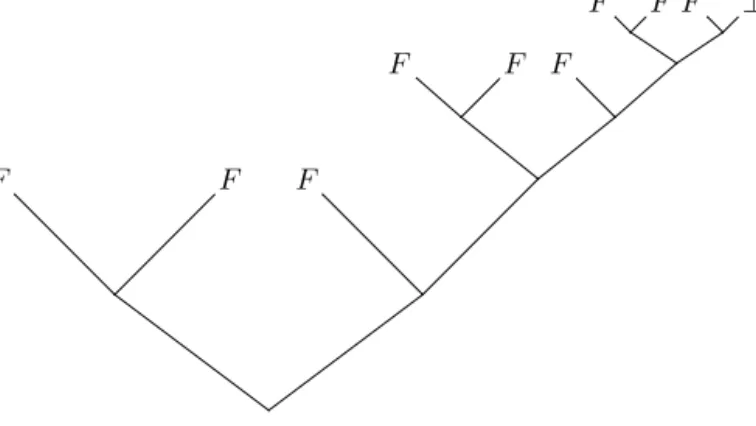
F F F ⊥
Fig. 1. One possible iteration of a simplified Miller-Rabin test on a composite number.
be used as an input tape for the Turing machine. It was shown that as long as p
is computable, then these machines cannot compute anything that a deterministic machine cannot compute. However, it may be possible that a probabilistic machine can compute something faster than any deterministic machine could [8].
Randomized computation first gained prominence when Rabin [6] introduced a randomized algorithm for finding the nearest pair in a set of npoints. This algo-rithm had a linear average runtime, faster than the nlogn runtime of the fastest known deterministic algorithm. More well known are the algorithms of Solovay and Strassen [21] and Rabin [17] for determining if a number is prime. These algorithms run in polynomial time (with a small error probability), and they were discovered over 20 years before the AKS primality test [3], the first known deterministic algo-rithm for recognizing prime numbers in polynomial time.
3
The Functor
This work is inspired by a model of uniform continuous random variables first pro-posed by Goubault-Larrecq and Varacca [9]. In their paper, it was shown that the category of bounded complete domains (BCD) is closed under a similar construc-tion. However, their assertion that the construction forms a monad in BCD was incorrect, since the proposed Kleisli extension failed to be monotone, thus not Scott continuous.
The basic idea of a random variable model is to separate the random choices from the domain itself. In the probabilistic powerdomain, the probability distributions are placed on the underlying domain. In a model of random variables, random bits are generated by coin flips, and then a random variable is defined from these random outcomes to the underlying domain. In the probabilistic powerdomain, for an element d, making a choice between d and d is the same as just d, since the probabilities are the same. In the model described here, there is a distinction between choosing d or d and d itself, even though the probabilities are the same. In the first case, a random bit is still chosen, so programmatically, this is distinct from the latter case where no such choice is made.
3.1 Motivation for the Functor
One of most well known randomized algorithms is the Miller-Rabin primality test. To test whether a given numbernis prime, a random number is chosen between 2
F F F
F F F
F F F ⊥
Fig. 2. Three iterations of a hypothetical Miller-Rabin test.
andn−2. Tests using modular arithmetic are performed with this random number before determining whether the given number is composite or probably prime. The test can be run in polynomial time, but has a possible one-sided error, putting primality testing in the complexity class of randomized polynomial time (RP). A test on a prime number will always return “probably prime”, but sometimes, a test on a composite number will also return “probably prime”. Thus, if the test returns “composite”, there is no chance for error, but a return of “probably prime” always has a chance of error. For a composite number, at most 1
4 of the possible random
choices between 2 and n− 2 will result in the test returning “probably prime”. To minimize the error probability, we can repeat the test (choosing a new random number) only when the test returns “probably prime”. Running the test m times results in an error probability of at most 41m.
Figure 1 shows the possible outcomes of a hypothetical Miller-Rabin test on a composite number. For simplicity, it is assumed that a random number between 2 and n−2 can be properly chosen using just two coin flips. Each coin flip is represented by a branching of the binary tree. The top of the tree is labeled with the return values of the test using the random numbers chosen by the resulting outcome of two coin flips. If the test returns “composite”, an “F” is used whereas “⊥” denotes “probably prime”. A “T” is not used since a Miller-Rabin test never confirms that a number is prime. If we wish to minimize the error probability, we can choose to run the test again, which will expand the tree wherever a “⊥” is found.
Figure 2 shows the possible outcomes of using Miller-Rabin a maximum of three times on the same composite number. This can be extended similarly to an infinite tree with a zero probability of error.
3.2 The Functor Definition
Let {0,1}∞ = {0,1}∗∪ {0,1}ω be the set of finite and infinite words of alphabet
{0,1}, with the prefix order (w ≤w if w is a prefix of w). The symbol ∗ is used to denote the concatenation operation. In this setting, a 0 represents getting tails on a coin flip, and a 1 signifies heads. If a fair coin is used, then for any word, the
probability associated with the word is 21n, wherenis the length of the word. For
example, the probability of 10, which represents getting heads and then tails, is 14.
Definition 3.1 An antichain of {0,1}∞ is a subset of words such that no two distinct words are comparable (no word is a prefix of another word). An antichain
M is full if ∀w ∈ {0,1}ω,∃z ∈ M, z ≤ w. Put another way, {0,1}ω ⊆ ↑M, or
M EM {0,1}ω. Denote the nonempty, full antichains by F AC({0,1}∞).
Using coin flips in a program results in a branching of computation that can be represented as a binary tree. The final possible outcomes will be located at the leaves of this tree, which must form an antichain. This antichain is required to be full since for any coin flip, it is possible to get either heads or tails, and both outcomes must be accounted for.
Definition 3.2 For a category of domains, the random choice functor, RC, is de-fined on objects by
RC(D) ={(M, f)| M ∈F AC({0,1}∞, f :M →D}
wheref is Scott continuous (givingM the subspace topology from the Scott topol-ogy of {0,1}∞). For a morphism, a:D→D, and (M, f)∈RC(D), we define
RC(a)(M, f) = (M, a◦f)
We order RC(D) by (M, f) (N, g) iff M EM N and w ≤ z ⇒ f(w)
g(z),∀w ∈ M, z ∈ N. Since the antichains are required to be full, M EM N is
equivalent to M ⊆ ↓N, or dually,N ⊆ ↑M. Another characterization for the order on functions is∀z∈N, f◦πM(z)g(z), whereπM(z) sendsz to the unique element
ofM belowz.
Theorem 3.3 IfD is a bounded complete domain, then so isRC(D).
4
The RC Monad
To show that the functor RC forms a monad, the unit and Kleisli extension (or multiplication) of the monad must be exhibited. For a domain D and d∈D, the unit,η:D→RC(D) is defined by
η(d) = (, χd)
where is the antichain only containing the empty word, and χd is the constant
function whose value isd.
4.1 Motivation for the Kleisli extension
The Kleisli extension of a monad T can be hard to think about intuitively since we normally do not work with functions from D to T(E). However, the Kleisli extension is important in lifting binary operations on the underlying structures
to binary operations on the monadic structures. If we have a binary operation
∗:D×E→F, the Kleisli extension lifts this operation to∗† :T(D)×T(E)→T(F). This is achieved by setting ∗†= (λa.T(λb.a∗b))†.
Suppose that we have a Miller-Rabin test performed on two composite numbers with the following possible outcomes:
F F F ⊥ ⊥ F F F
How should the binary operation orbe lifted? It may seem natural to perform the two tests one after the other, resulting in:
⊥ F F F ⊥ F F F ⊥ F F F ⊥ ⊥ ⊥ ⊥
The probability of error in this case is 167, assuming we use a fair coin. However, this method has two main flaws.
(i) How do we handle the infinite case? If the first random test can use infinitely many coin flips, then the second test will never even start.
(ii) The Kleisli extension that results in this behavior is not monotone. Therefore, it does not form a monad in a category we want.
Instead, consider feeding the result of each coin flip to both tests concurrently. For two coin flips, our example would look like:
⊥ F F ⊥
To properly compare it with the sequential case, we should use the same max-imum number of coin flips. Feeding all four coin flips to both Miller-Rabin tests results in:
F F
⊥ F F F F F F ⊥
which only has an error probability of 18. If the error possibility for each number had coincided, then the error probability would have been smaller, 161.
It some cases, it may be desirable to have two random processes run sequen-tially instead of the concurrent behavior described here. However, for a randomized algorithm like Miller-Rabin, which has a fixed desired output, this is unnecessary. These algorithms are represented by possibly infinite trees that have a zero error probability. Combining these trees as described above results in another tree with a zero error probability. In fact, the error probability can decrease more quickly using this method. But if it is necessary to have a sequential composition of random processes, then we must move outside of the RC monad to accomplish this. We can create a function on RC(D)×N that takes a random process and uses ncoin flips to output an element ofD. This function is not deterministic, so the output would need to be in T(D) for some other monad T. For example, in Haskell, we can use the standard random library to simulate coin flips, andT in this case would be Haskell’s IO monad. Composing two such actions would result in the random choices occurring sequentially. More generally, we can use a probabilistic monad such as the indexed valuations or finite random variables as the codomain of this function.
4.2 Kleisli Extension of the Monad
Consider h : D → RC(E). For an element (M, f) ∈ RC(D), each w represents one possible outcome of coin flips. For each w, h◦f(w) gives another randomized algorithm, in RC(E). Thus, there is a random choice of random algorithms, and the Kleisli extension has to convert this into one randomized algorithm in (N, g)∈
RC(E). Instead of using all ofh◦f(w), for eachw, we use the coin flips represented bywand feed them intoh◦f(w). If the first coin flip was “heads” moving towards
w, then we assume that the first coin flip will be “heads” when running h◦f(w). Thus, our extension only considers the part of π1◦h◦f(w) that is on the same
“branch” of the tree asw, namely ↑w∪ ↓w.
Definition 4.1 For (M, f)∈RC(D), the first component of the Kleisli extension,
π1◦h†(M, f) will give an antichain that is bigger than the originalM. It is defined
as follows:
π1◦h†(M, f) =
w∈M
where Min(W) gives the minimal words ofW. The second component of the Kleisli extension gives a function from the first component into E. For a given z in the first component, this is defined by:
((π2◦h†)(M, f))(z) =g(πN(z)) where (N, g) =h◦f◦πM(z)
Since the first component given by the Kleisli extension is bigger than M, the function f may not be defined on z. Therefore,πM(z) is used followed byh◦f to
pick a randomized algorithm (N, g) ∈RC(E). Similarly, g may not be defined on
z, but there is a unique element of N, πN(z), where it is defined.
Proposition 4.2 h† is monotone.
Proof. (M, f) ≤ (N, g) means that N ⊆ ↑M (thus, ↑N ⊆ ↑M) and w ≤ z ⇒ f(w)≤g(z) for anyw ∈M, z∈N. ↑π1◦h†(M, f) =↑ w∈M Min(↑w ∩ ↑π1◦h◦f(w)) = w∈M ↑Min(↑w ∩ ↑π1◦h◦f(w)) = w∈M (↑w ∩ ↑π1◦h◦f(w))
The same applies to (N, g), so we just need to show that
z∈N (↑z ∩ ↑π1◦h◦g(z))⊆ w∈M (↑w ∩ ↑π1◦h◦f(w))
For each z ∈ N, there is a w ∈ M that is below z. In this case, ↑z ⊆ ↑w and
↑(π1◦h◦g(z)) ⊆ ↑(π1◦h◦f(w)) since g(z) ≥ f(w) and h is monotone. Thus,
(↑z ∩ ↑(π1◦h◦g(z)))⊆(↑w ∩ ↑(π1◦h◦f(w))).
Now we check the functions. For w ∈ (π1◦h†(M, f)) and z ∈ (π1◦h†(N, g))
with w≤z, we must show that (π2◦h†(M, f))(w)≤(π2◦h†(N, g))(z).
LetπM(w) equal the unique word inM beloww. Sincew≤z,πM(w)≤πN(z),
andf◦πM(w)≤g◦πN(z). Sinceh is monotone, h◦f◦πM(w)≤h◦g◦πN(z).
Again, since w≤z, ππ1◦h◦f◦πM(w)(w)≤ππ1◦h◦g◦πN(z)(z), and we have (π2◦h†(M, f))(w) = (π2◦h◦f◦πM(w))(ππ1◦h◦f◦πM(w)(w))
≤(π2◦h◦g◦πN(z))(ππ1◦h◦g◦πN(z)(z))
= (π2◦h†(N, g))(z)
2 Proposition 4.3 h† is Scott continuous.
5
Distributive Laws and Extending the Monad
One of the downsides with the probabilistic powerdomain is that it does not satisfy a distributive law with any of the nondeterministic powerdomains. However, we can show that our monadRC does satisfy a distributive law with respect to the lower powerdomain in the category BCD.
For two monads, (S, ηS, μS) and (T, ηS, μS), over the same category, the functor
T S is not necessarily a monad. According to Beck’s Theorem [4], the composition of two monads,SandT, is a monad if and only if there is a distributive law between them. A distributive law consists of a natural transformation λ : ST → T S that satisfies the following equations:
(i) λ◦SηT =ηTS
(ii) λ◦ηST =T ηS
(iii) λ◦SμT =μTS◦T λ◦λT
(iv) λ◦μST =T μS◦λS◦Sλ
5.1 Distributive Law With the Lower Powerdomain
Let ΓL be the lower powerdomain functor. Suppose (M, f) ∈ RC ◦ΓL(D), so
that f is a function from M to ΓL(D). Now define the natural transformation
λ:RC◦ΓL(D)→ΓL◦RC(D) by:
λ(M, f) =↓{(M, g)| g(w)∈f(w),∀w ∈M}
Proposition 5.1 There is a distributive law between the monad of random choice and the lower powerdomain, using the natural transformation λ.
5.2 Extending the Monad
The above construction is a monad in the categoryBCD. However, only two of the nondeterministic powerdomains (the upper and lower) leave BCD invariant. BCD is not closed under the convex powerdomain, but the Cartesian closed categories
RBandFS, which contain BCD, are. The monadRC is not believed to stay within these categories, since we see no way to construct the deflations needed to show that an object is in one or the other of these categories. In BCD, infima can be used, but outside of BCD, infima are not guaranteed. One way to repair this is to not only define our functions on antichains, but instead to define them on the Scott closure, or lower set, of these antichains. This way, there is no need for infima to project down to smaller trees, since the function is already defined on the lower set. In our first monad, antichains are used, representing the possible outcomes of a random computation. Now we change this monad to include not only antichains of words, but also the prefixes of these words. These prefixes represent intermediate stages of computation where more random bits are still needed.
Definition 5.2 A Scott closed set M in {0,1}∞ isfull if for all words, w, in M,
of{0,1}∞ by Γf({0,1}∞).
Γf({0,1}∞), ordered by inclusion, is a subposet of the lower powerdomain of
{0,1}∞. If a poset is a dcpo, domain, or bounded complete domain, then so is the lower powerdomain of that poset. The supremum of some nonempty subset {Mi}
is simply the closure of the union, iMi.
Definition 5.3 For a category of domains, the functor RC is now defined on objects by
RC(D) ={(M, f) |M ∈Γf({0,1}∞), f :M →D is Scott continuous}
For a:D→D and (M, f)∈RC(D), we define
RC(a)(M, f) = (M, a◦f)
RC(D) is given an order such that (M, f) (N, g) iff M ⊆ N and f(w) ≤
g(w),∀w∈M.
Theorem 5.4 RC is an endofunctor in the categoriesRB and FS.
For the monad construction, the unit is the same as before:
η(d) = (, χd)
For a continuous function h:D→RC(E) and some (M, f) in RC(D), the Kleisli extension is defined by π1◦h†(M, f) =M ∪( w∈M (↑w∩(π1◦h◦f(w)))) ((π2◦h†)(M, f))(z) =g(πN(z)) where (N, g) =h◦f◦πM(z).
Theorem 5.5 The functor RC forms a monad in the categoriesRB and FS. 5.3 Distributive Law With the Convex Powerdomain
Let ΓC denote the convex powerdomain functor. Recall that the convex
powerdo-main of a coherent dopowerdo-main D consists ofLens(D), the nonempty lenses of D. For a nonempty compactK ⊆D, define thelens closure ofK byK=K ∩ ↑K. The lens closureK is the smallest lens containingK.
Suppose U ∈ΓC◦RC(D), so that U is a lens of random choices ofX. Define
the natural transformation, λ: ΓC◦RC(D)→RC◦ΓC(D) by:
λ(U) = (
(M,f)∈U
M , w→
(M,f)∈U
f◦πM(w))
Proposition 5.6 There is a distributive law between the monad of random choice and the convex powerdomain, using the natural transformation λ.
6
Relation to Scott’s Stochastic Lambda Calculus
Dana Scott developed an operational semantics of the lambda calculus using the power set of the natural numbers,P(N). As terms of the lambda calculus, elements of P(N) can be applied to one another and λ-abstraction is achieved through the use of enumerations similar to G¨odel numbering.
Scott then added randomness to his model, resulting in his stochastic lambda calculus [20]. He does this by adding random variables.
Definition 6.1 Arandom variable in Scott’s model is a functionX: [0,1]→ P(N) where{t∈[0,1]|n∈X(t)}is Lebesgue measurable for allnin P(N).
This is similar to the monad of random choice presented in this paper. We start with a base domain D, which could be P(N), and then have a function from an antichain of{0,1}∞ intoD. We can really treat this as a function from the Cantor space,{0,1}ω toD. For some (M, f), definef :{0,1}ω→D byf(z) =f(πM(z)).
Now that random variables are added to the lambda calculus, there must be a way to define application of one random variable to another. In a sense, this is lifting the application operation from P(N)× P(N) to ([0,1] → P(N))×([0,1] → P(N)), which, as stated above, is the role of the Kleisli extension of the monad. Scott defines the application as follows:
Definition 6.2 Given two random variablesX,Y : [0,1] → P(N), the application operation is defined by
X(Y)(t) =X(t)(Y(t))
These random variables can be thought of as using an oracle that randomly gives a element of [0,1], and then the function of the random variable uses this number to output an element of P(N). Notice that in the above definition for application, both random variables receive the samet. Thus, the oracle is consulted only once instead of giving a different random number to each random variable. This exactly mimics the concurrent operation of our Kleisli extension. But instead of an oracle giving an entire real number at once (which has infinite information), the oracle gives one bit at a time.
7
Summary and Future Work
In this paper, we have a presented two monads for randomized computation in Cartesian closed categories of domains. Computational motivation is given for the structure of these monads. In a program, random choice results in the branching of computation, so the possible outcomes form a tree. Our first monad separates random choice from the underlying domain and confines it to the leaves of a binary tree. This is the main difference between our construction and the probabilistic powerdomain. We have shown that this monad captures the randomized behavior found in algorithms such as the Miller-Rabin primality test. We have given a new Kleisli extension that satisfies the monad laws and presented a distributive law with the lower powerdomain, all within the categoryBCD. In order to work with the
convex powerdomain, we needed to move into the categoryRBorFS. A slight change was needed for our construction to stay within these categories, and a distributive law was given between this extended monad and the convex powerdomain.
There is much work to be done concerning these monads. Some work has al-ready been completed that is beyond the scope of this paper. Another alteration can be made to the monad to obtain a distributive law with the upper powerdomain. Furthermore, an operational version of the monad has been developed and imple-mented in functional programming languages such as Scala and Haskell. The proof that the monad laws hold for this operational version has been formally verified us-ing Isabelle. Finally, Randomized PCF (rPCF), a programmus-ing language that adds random choice to PCF [19], has been designed, and the Miller-Rabin algorithm has been implemented within the language. An operational and denotational semantics for rPCF have been developed using the monad presented in this paper. This is a proof of concept to show how this monad can be used to augment other languages with random choice.
8
Acknowledgements
The author thanks Michael Mislove for the guidance and the many fruitful discus-sions that made this work possible, along with several much-needed suggestions for the preparation of this paper. The author also thanks Jean Goubault-Larrecq and Dana Scott for email correspondence regarding the model of continuous random variables and the stochastic lambda calculus, respectively. Finally, the author ac-knowledges the support of the AFOSR under award no. FA0550-13-1-0135 during the preparation of this work.
References
[1] Abramsky, S. and A. Jung,Domain theory, Handbook of logic in computer science3(1994), pp. 1–168. [2] Abramsky, S. and N. Tzevelekos,Introduction to categories and categorical logic, in:New structures
for physics, Springer, 2011 pp. 3–94.
[3] Agrawal, M., N. Kayal and N. Saxena,Primes is in p, Annals of mathematics (2004), pp. 781–793.
[4] Beck, J.,Distributive laws, in:Seminar on triples and categorical homology theory, Springer, 1969, pp. 119–140.
[5] De Leeuw, K., E. F. Moore, C. E. Shannon and N. Shapiro,Computability by probabilistic machines, Automata studies34(1956), pp. 183–198.
[6] Division, I. B. M. C. R. and M. Rabin, “Probabilistic algorithms,” 1976.
[7] Gierz, G., K. H. Hofmann, K. Keimel, J. D. Lawson, M. Mislove and D. S. Scott,Continuous lattices and domains, volume 93 of encyclopedia of mathematics and its applications(2003).
[8] Gill, J.,Computational complexity of probabilistic turing machines, SIAM Journal on Computing 6 (1977), pp. 675–695.
[9] Goubault-Larrecq, J. and D. Varacca,Continuous random variables, in:Proceedings of the 26th Annual IEEE Symposium on Logic in Computer Science (LICS’11)(2011), pp. 97–106.
URLhttp://www.lsv.ens-cachan.fr/Publis/PAPERS/PDF/GLV-lics2011.pdf
[11] Jung, A. and R. Tix, The troublesome probabilistic powerdomain, Electronic Notes in Theoretical Computer Science13(1998), pp. 70–91.
[12] Mislove, M., Nondeterminism and probabilistic choice: Obeying the laws, in: CONCUR 2000 Concurrency Theory, Springer, 2000 pp. 350–365.
[13] Mislove, M., Discrete random variables over domains, Theoretical computer science 380 (2007), pp. 181–198.
[14] Mislove, M.,Anatomy of a domain of continuous random variables ii, in:Computation, Logic, Games, and Quantum Foundations. The Many Facets of Samson Abramsky, Springer, 2013 pp. 225–245.
[15] Mislove, M. W., Topology, domain theory and theoretical computer science, Topology and its Applications89(1998), pp. 3–59.
[16] Moggi, E.,Notions of computation and monads, Information and computation93(1991), pp. 55–92. [17] Rabin, M. O.,Probabilistic algorithm for testing primality, Journal of number theory12(1980), pp. 128–
138.
[18] Saheb-Djahromi, N.,Cpo’s of measures for nondeterminism, Theoretical Computer Science12(1980), pp. 19–37.
[19] Scott, D. S.,A type-theoretical alternative to ISWIM, CUCH, OWHY, Theoretical Computer Science
121(1993), pp. 411–440.
[20] Scott, D. S.,Stochasticλ-calculi, Journal of Applied Logic12(2014), pp. 369–376.
[21] Solovay, R. and V. Strassen,A fast monte-carlo test for primality, SIAM journal on Computing6 (1977), pp. 84–85.
[22] Tix, R., “Continuous D-cones: convexity and powerdomain constructions,” Shaker, 1999.
[23] Tix, R., K. Keimel and G. Plotkin,Semantic domains for combining probability and non-determinism, Electronic Notes in Theoretical Computer Science222(2009), pp. 3–99.
[24] Varacca, D., “Probability, nondeterminism and concurrency: two denotational models for probabilistic computation,” BRICS, 2003.
[25] Varacca, D., G. Winskel et al.,Distributing probability over non-determinism, Mathematical Structures in Computer Science16(2006), pp. 87–113.