Bayesian Estimation of Multivariate Conditional Correlation GARCH models and Their Application

(1)

Bayesian Estimation of Multivariate Conditional

Correlation GARCH models and Their Application

Chen Jun

Master’s degree Programme in Bayesian Statistics and Decision Analysis (EuroBayes)

Department of Mathematics and Statistics University of Helsinki

(2)

Tiedekunta/Osasto Fakultet/Sektion – Faculty Faculty of Science

Laitos/Institution– Department

Department of Mathematics and Statistics Tekijä/Författare – Author

Chen Jun

Työn nimi / Arbetets titel – Title

Bayesian Estimation of Multivariate Conditional Correlation GARCH models and Their Application Oppiaine /Läroämne – Subject

Master’s degree Programme in Bayesian Statistics and Decision Analysis Työn laji/Arbetets art – Level

Master's thesis

Aika/Datum – Month and year November 2015

Sivumäärä/ Sidoantal – Number of pages

63 Tiivistelmä/Referat – Abstract

The thesis studies three different conditional correlation Multivariate GARCH (MGARCH) models. They are the Constant Conditional Correlation (CCC-) GARCH, Dynamic Conditional Correlation (DCC-) GARCH and Asymmetric Dynamic Conditional Correlation (ADCC-) GARCH, in which the time-varying volatilities are modelled by three univariate GARCH models with the error term assumed to have a Gaussian distribution. In order to compare the performance of these models, we apply them to the volatility analysis of two stocks. Regarding model inference, we adopt a Bayesian approach and implement a Markov Chain Monte Carlo (MCMC) algorithm, Metropolis Within Gibbs (MWG), instead of the regular maximum likelihood (ML) method. Finally, the estimated models are employed to compute Value at Risk (VaR) and their performance is discussed.

Avainsanat – Nyckelord – Keywords

CCC-GARCH, DCC-GARCH, ADCC-GARCH, MCMC

Säilytyspaikka – Förvaringställe – Where deposited Kumpula science library

(3)

The thesis studies three diﬀerent conditional correlation Multivariate GARCH (MGARCH) models. They are the Constant Conditional Correlation (CCC-) GARCH, Dynamic Con-ditional Correlation (DCC-) GARCH and Asymmetric Dynamic ConCon-ditional Correlation (ADCC-) GARCH, in which the time-varying volatilities are modelled by three univariate GARCH models with the error term assumed to have a Gaussian distribution. In order to compare the performance of these models, we apply them to the volatility analysis of two stocks. Regarding model inference, we adopt a Bayesian approach and implement a Markov Chain Monte Carlo (MCMC) algorithm, Metropolis Within Gibbs (MWG), instead of the regular maximum likelihood (ML) method. Finally, the estimated models are employed to compute Value at Risk (VaR) and their performance is discussed.

(6)

Chapter 1 Introduction

Albeit the volatility, which is a significant feature in financial time series, has been stud-ied for several decades, the interest in it has no signs of fading. Instead, because of the increase in complexity of financial instruments, e.g. option pricing, volatility is attracting even more attention today.

A well-known property of volatility is heteroscedasticity, which is referred to the phe-nomenon of time-varying volatility clustering, i.e., periods of large volatility and periods of small volatility tend to appear continuously. To capture such a character in financial time series, Engle [9] introduced the Autoregressive Conditional Heteroscedasticity (ARCH) model. Whereafter, Bollerslev [3] extended the ARCH model into General Autoregressive Conditional Heteroscedasticity (GARCH) model, which achieved a huge success in mod-elling heteroscedasticity in financial time series. More significantly, it laid the foundation for succedent research in this topic and various extensions of the GARCH model have been developed, including, the GJR-GARCH model by Glosten, Jagannathan and Runkle [13], and the Exponential GARCH (EGARCH) model of Nelson [18].

(7)

As we usually consider a portfolio of assets and make decisions regarding the portfolio, it is essential to study the volatilities between the assets in the portfolio simultaneously. A solution is to use univariate GARCH models to describe volatilities of each individual asset and construct the covariance matrix between the assets. This is the basic idea used to develop a Multivariate GARCH (MGARCH) model where main challenge is to make the model suﬃciently flexible and yet parsimonious.

Of the multivariate GARCH models proposed the VEC-GARCH model of Bollerslev, Engle, and Wooldridge [5] and its restricted version the BEKK model of Engle and Kro-ner [10] are flexible but not parsimonious. In this thesis we therefore consider multivariate GARCH model based on the conditional correlations.

In 1990, Bollerslev [4] introduced a multivariate GARCH model, referred as the Constant Conditional Correlation (CCC-) GARCH model, in which univariate GARCH models re-lated to one another with a constant correlation matrix. In his Dynamic Conditional Correlation (DCC-) GARCH models, Engle [8] relaxed the assumption of a constant cor-relation by allowing for time varying corcor-relations. A further extension is the Asymmetric Dynamic Conditional Correlation (ADCC-) GARCH model proposed by Cappiello, Engle and Sheppard [6] with the motivation of allowing for asymmetric impacts on the correla-tions caused by good news and bad news.

Generally, the classical approach of estimating the parameters of GARCH models is the method of ML. However, in this thesis a Bayesian approach: Markov Chain Monte Carlo (MCMC) method is applied. Ardia and Hoogerheide [1] outline the MCMC method for GARCH models. Of various MCMC algorithms applied in the estimation of GARCH models, Tetsuya Takaishi [21] employed the Hamilton Monte Carlo algorithm and Ar-dia [2] used Metropolis Hasting scheme in GARCH(1,1) with Student-tinnovations. They demonstrated the MCMC method can be very useful in estimating GARCH models. This thesis consists of the following chapters: In Chapter 2 and Chapter 3, the

(8)

uni-variate GARCH models and multiuni-variate GARCH models considered in the thesis are introduced. In Chapter 4, Bayesian estimation is discussed in the context of multivariate GARCH models. In Chapter 5, CCC-GARCH, DCC-GARCH and ADCC-GARCH mod-els are built for two stocks, General Electric and American Express Company, and applied in Chapter 6 to estimate VaR. Finally, conclusions are provided in Chapter 7.

(9)

Chapter 2 Univariate Models

2.1 Symmetric Models

2.1.1 ARCH Model

The traditional assumption that the one-period forecast error variance is constant across all the time points in a series does not reflect the existence of time varying variance ob-served in stock returns. To allow for this feature, Engle [9] introduced the autoregressive conditional heteroskedasticity (ARCH) model. The ARCH model assumes that condi-tional variances given the past information are non-constant described by a function of previous squared returns. The definition of the qth order ARCH model, ARCH(q) for short, is given in the following definition:

(10)

Definition 2.1.1. The ARCH(q) model is defined by the equations rt=µt+yt (2.1) yt= p htzt, (2.2) ht=!+ q X i=1 ↵iy2_{t i}, (2.3) where

• rt is the considered return at time t; • µt is the expected return at time t; • yt is the mean corrected return at time t;

• zt is a sequence of independent and identical distributed (i.i.d.) with zero mean and

unit variance, such that zt is independent of (rt 1, rt 2, . . .);

• htis the conditional variance of the return at timetgiven the past returns(rt 1, rt 2, . . .);

• ! > 0 and ↵i 0 are parameters used to specify the conditional variance ht with

the inequalities guaranteeing that ht is positive;

In Equation (2.1), µt could be time varying and modelled by some time series model, e.g.,

an autoregressive model. However, because our main object is to study the volatility, we assume that µis constant and equal to the mean of the series. In Equation (2.2), zt

is transformed into yt by multiplying with p

ht, and from the assumption on zt made it

follows that ht defined in (2.3) is the conditional variance of the returns. Thus the model

describes the heteroskedasticity observed in reality.

From the definition of the ARCH model, it is explicit that for ↵i > 0, a large value of a

squared past return y2

t i results in a large conditional variance htand the probability that

(11)

the clustering phenomenon observed in financial time series. After the introduction of the ARCH model, its useful in describing time varying volatility was established in numerous applications.

2.1.2 GARCH Model

Although the ARCH model made extraordinary progress in the analysis of time varying volatility, it has some limitations. Tsay [23] showed that it often requires many lags to describe the volatility adequately, i.e., q in Equation (2.3) should be large. In 1986, Tim Bollerslev [3] introduced an extension, the Generalized Autoregressive Conditional Het-eroskedasticity (GARCH) model, in which the conditional variance is not only explained by past squared returns but also by past conditional variances, thereby allowing for a more flexiblility.

Definition 2.1.2. The definition of the GARCH(p, q) is defined by the equations:

rt=µt+yt, (2.4) yt= p htzt, (2.5) ht=!+ p X i=1 ↵iy_{t i}2 + q X i=1 iht i, (2.6)

where, rt, µt, yt andztare as in the definition of the ARCH model (See Definition 2.1.1).

In the GARCH model, ht is explained by both squared past returns yt i2 and past

condi-tional variances ht i. To ensureht is greater than zero, ! >0and ↵i, i 0 are assumed

and if ↵i = 0 for all i, then i = 0 for all i must hold. Empirical experience has shown

that less free parameters are needed in the GARCH model than in the ARCH model to describe the volatility of the same asset return, and consequently the GARCH model has been used more widely in practice than the ARCH model [23].

(12)

2.2 Asymmetric Models

In financial markets, the leverage effect is used to refer to the unequal effect caused by bad news and good news. To allow for the leverage effect, extensions of the GARCH model have been developed, including the EGARCH model of Nelson [18], the NGARCH model of Engle and Ng [11] and the Threshold GARCH model of Zakoian [24]. In the thesis, we selected two asymmetric GARCH models, the QGARCH model of Sentana [20] and the GJR-GARCH model of Glosten, Jagannathan and Runkle [13] are considered.

2.2.1 QARCH Model

The QGARCH model is short for the Quadratic GARCH model proposed by Sentana [20]. Unlike the conventional GARCH model, the QGARCH model allows the conditional vari-ance to depend not only on squared returns but also on the returns. A formal definition of the QGARCH model is as follows

Definition 2.2.1. The definition of the QGARCH(p, q) is defined by the equations:

rt=µt+yt (2.7) yt= p htzt (2.8) ht=!+ p X i=1 ↵iiy2t i+ p X i=1 iyt i+ 2 p X i=1 p X j=i+1 ↵ijyt iyt j+ q X i=1 iht i (2.9)

where, rt, µt, yt and zt are as in the definition of the ARCH model (See Definition 2.1.1).

As seen in Equation (2.6) and Equation (2.9), the QGARCH model contains the extra part Pp

i=1 iyt i+ 2

Pp i=1

Pp

j=i+1↵ijyt iyt j not appearing in the GARCH model.

(13)

vector form as ht=!+Y0t 1AYt 1+ 0Yt 1+ q X i=1 iht i. (2.10) = (Y0t 1,1) 2 4A 2 2 0 ! 3 5 0 @Yt 1 1 1 A+ q X i=1 iht i, (2.11)

where is a p_⇥1 vector with the components 1, . . . , p and A is a symmetric p⇥p

matrix with elements ↵i,j = ↵j,i. To satisfy the positivity assumption of the conditional

variance ht, we require ! >0, i 0, and that the matrices

2 4A 2 2 0 ! 3

5 _and A are positive semidefinite. If A+ _{denotes the Moore-Penrose inverse of} _{A, the non-negativity of the is}

guaranteed by the inequality ! 0_A+ _/₄ ₀ _[20].

With the purpose to have a parsimonious model, we always treat the matrix A as a

diagonal matrix in which case the conditional variance in Equation (2.9) simplies to ht =!+ p X i=1 ↵iiy_{t i}2 + p X i=1 iyt i+ q X i=1 iht i (2.12)

To see how the QGARCH model works, consider Equation(2.12), where the coeﬃcient

i shows the diﬀerence to the GARCH model. As usual assume that bad news brings

negative mean corrected returns y_{t i} and good news brings positive returnsy_{t i}+ . Then if

iis negative, the inequality iyt i> iyt i+ is satisfied, and it follows from Equation (2.12)

that the negative returny_{t i}has a greater impact on the volatility than a positive returns y_{t i}+ .

2.2.2 GJR-ARCH Model

Another model widely used to describe the leverage eﬀect is the GJR-GARCH model, it is named after Glosten, Jagannathan, and Runkle [13] and defined as follows.

(14)

Definition 2.2.2. The GJR-GARCH(p,q) model is defined by the equations rt=µt+yt (2.13) yt= p htzt, (2.14) ht=!+ p X i=1 ↵iy_{t i}2 + p X i=1 iIi[yt i<0]yt i2 + q X i=1 iht i (2.15)

where, rt, µt, yt and zt are as in the definition of the ARCH model (See Definition 2.1.1)

and Ii[yt i <0] = 8 > < > : 1 if yt i<0 0 if yt i 0 (2.16)

From the definition of GJR-GARCH model, it is seen a negative mean corrected return yt i caused by bad news will aggrandise the conditional variance ht by iy2t i.

Compared to the QGARCH model, the GJR-GARCH model has the advantage that the restrictions on the parameters needed to guarantee positive conditional variance are rela-tive simpler, only! >0and that all other parameters are non-negative will suﬃce.

(15)

Chapter 3 Multivariate Models

Generally, financial returns move simultaneously over time across diﬀerent assets or mar-kets and their comovement are dependent on their covariance structure. Consequently, in empirical analyses, especially in financial risk management, studying the volatilities with multivariate models is more relevant than working with univariate models separately. Before presenting specific multivariate GARCH models, we describe the general structure used in the definition.

Definition 3.0.1. The general structure of models for multivariate conditional het-eroskedasticity is given by the equations

rt=µt+yt (3.1)

yt=H1t/2zt (3.2)

where

• rt is the n⇥1 vector of returns at timet;

(16)

• yt is the n⇥1 vector of mean corrected returns at time t;

• zt is an⇥1sequence of i.i.d random vectors with zero mean and identity covariance

matrix and such that zt is independent of past returns (r1,r2, . . .);

• Ht is then⇥n conditional covariance matrix of the returns at timet given the past

returns (r1,r2, . . .).

The Equation (3.1) and Equation (3.2) have obvious counterparts in the univariate models discussed in previous chapters. For example, the vector µt contains the expected returns

and Ht is a multivariate extension of the conditional covariance. To complete the

speci-fication of the model, the conditional covariance matrix Ht should be specified.

As mentioned in the Introduction, examples of the specifications proposed in literature, include the VEC model [5] and the BEKK model [10]. But in the thesis, multivariate conditional correlation models will be considered.

In the multivariate conditional correlation volatility models, the conditional covariance matrix Ht is specified in a two-step way. Firstly, one specifies the conditional variances

separately for each returns by using a univariate GARCH model. For instance, the con-ditional variances could follow a GARCH model or a QGARCH model if allowance of asymmetric eﬀects is desired. Whereafter, the conditional variances specified in the first step are used to build the conditional covariance matrix Ht. So the following sections we

discuss the multivariate conditional correlation mocels, namely the Constant Conditional Correlation model, the Dynamic Conditional Correlation model and the Asymmetric Con-ditional Correlation model.

(17)

3.1 Constant Conditional Correlation Model

The Constant Conditional Correlation (CCC) GARCH model was first put forward by Bollerslev [4]. It is the simplest model among the three models to be discussed. The key assumption is that the conditional correlations between the elements of yt are time

invariant.

Definition 3.1.1. Given the Definition 3.0.1, the specification of Ht in CCC-GARCH

model is given by equations

Ht=D1t/2RD

1/2

t (3.3)

Dt=diag(h11,t, . . . , hnn,t) (3.4)

where

1. Dt is a diagonal matrix with positive diagonal entries that are the conditional

vari-ances specified by univariate GARCH models; 2. R is a positive definted correlation matrix, i.e.,

R= 0 B B B B B @ 1 ⇢12 . . . ⇢1n ⇢21 1 . . . ⇢2n ... ... ... ... ⇢n1 ⇢n2 . . . 1 1 C C C C C A (3.5)

In Definition 3.0.1, Ht is required to be positive definite. In the CCC-GARCH model,

this condition is guaranteed by the requirement R and Dt are positive definite, this

particularly means that all conditional variances must be positive so that the constrains for positive conditional variance should be satisfied for each univariate GARCH model. From Equation (3.3), we have

hij,t=⇢ij ·

p

(18)

and when R equals the identy matrix I so that ⇢ij = 0 when i 6= j, we get the special

case where all assets are independent with conditional variances modeled by univariate GARCH models.

3.2 Dynamic Conditional Correlation Model

Compared to other multivariate GARCH models, the CCC-GARCH model reduces the number of free parameters. However, the assumption of constant conditional correlation is restrictive in most empirical applications. This leads to Engle’s [8] the Dynamic Con-ditional Correlation (DCC)-GARCH model, in which the correlation matrix R is time variant.

Definition 3.2.1. Given Definition 3.0.1, the specification of Ht in the DCC-GARCH

model is given by the equations

Ht=D1t/2RtD1t/2 (3.7) Dt=diag(h11,t, . . . , hnn,t) (3.8) Rt=diag(q111,t/2, . . . , q 1/2 nn,t )Qtdiag(q111,t/2, . . . , q 1/2 nn,t ) (3.9) Qt= (1 a b) ¯Q+a✏t 1✏0t 1+bQt 1 (3.10) where

1. Dt is as in the CCC-GARCH model (see Definition 3.1.1);

2. Rt is the time-varying correlation matrix

Rt = 0 B B B B B @ 1 ⇢12,t . . . ⇢1n,t ⇢21,t 1 . . . ⇢2n,t ... ... ... ... ⇢n1,t ⇢n2,t . . . 1 1 C C C C C A (3.11)

(19)

and qii,t in Equation (3.9) is the ith diagonal element of the symmetric matrix Qt

with typical element qij,t

3. ✏t is a standardised residual vector with component ✏i,t =yi,t/

p hii,t;

4. _Q¯ _{is a positive definite parameter matrix with unit diagonal elements.}

According to the Equation (3.9) and Equation (3.10), the correlation matrix Rt is

con-structed through the matrix Qt. In addition to a well defined conditional variances, the

scalar parameters a, b need to be non-negative and satisfy a +b < 1 to guarantee Qt

is positive definite and consequently Rt is positive. Positive constraints on Dt and Rt

ensure the postive definte of Ht.

3.3 Asymmetric Dynamic Conditional Correlation Model

Similar to asymmetries in volatility, asymmetric eﬀect also exists in the conditional cor-relations. This feature can be captured by the Asymmetric DCC-GARCH model of Cap-piello, Engle and Sheppard [6].

Definition 3.3.1. Given Definition 3.0.1, the specification of Ht in the ADCC-GARCH

model is given by the equations

Ht =D1t/2RtD1t/2 (3.12) Dt =diag(h11,t, . . . , hnn,t) (3.13) Rt =diag(q111,t/2, . . . , q 1/2 nn,t )Qtdiag(q111,t/2, . . . , q 1/2 nn,t ) (3.14) Qt = ( ¯Q A0QA¯ B0QB¯ G0NG¯ ) +A0✏t 1✏0t 1A+B0Qt 1B+G0nt 1n0t 1G (3.15)

where the quantities in Equation (3.12), Equation (3.13) and Equation (3.14) are as the DCC-GARCH model (see Definition 3.2.1 ). In Equation (3.15),

(20)

1. nt=I[✏t<0] ✏t( is the Hadamard product) with the ithe component of then⇥1 vector I[✏t <0]defined as Ii[✏i,t <0] = 8 > < > : 1 if ✏i,t <0 0 if ✏i,t 0 (3.16)

2. A, B and G are diagonal parameter matrices. 3. _N¯ _{is a positive semidefinite parameter matrix.}

In order to guarantee that the conditional covriance matrix Ht is positive definite, the

constraints on the matrix Dt and Rt should be the same as in DCC-GARCH model. In

the ADCC-GARCH model, as Rt needs to be positive definite, matrix Qt needs to be

positive definite, and therefore the follong condition should be hold:

¯

Q AA0 Q¯ BB0 Q¯ GG0 N¯ (3.17)

is positive definite.

With the purpose to reduce the dimension of the parameter vector but still keep the flexibility of the model, we adopt a special case and replace the coeﬃcient matrix A, B, G by scalars pa, pb and pg. Then the Equation (3.15) can be rewritten as

Qt= ( ¯Q aQ¯ bQ¯ gN¯) +a✏t 1✏0t 1+bQt 1+gnt 1nt 1 (3.18)

and the condition for positive definition of Qt can be rewritten as: a+b+ g <1, where

(21)

Chapter 4 Model Estimation

In this chapter, we describe the scheme used to estimate parameters of the models in-troduced in the preceding chapters. A essential assumption is that the standard error zt

follows a standardised multivariate Gaussian distribution.

4.1 Log likelihood function

When the standardised errorztis from a multivariate Gaussian distribution with E[zt] = 0

and Var[zt] =I, the joint distribution of an independent sample z1, . . . ,zT is:

f(z1, . . . ,zT) = T Y i=1 1 (2⇡)n/2exp( 1 2z 0 tzt) (4.1)

According to Definition 3.0.1, we assume that the expected return µt equals a constant

so that rt =µ+yt. To simplify notation, we assume in this chapter that µ= 0and use

the notation yt for the vector of returns.

(22)

Var[yt] =Ht and the joint distribution of y1, . . . ,yT is: f(y1, . . . ,yT) = T Y i=1 1 (2⇡)n/2_|_H_t|1/2 exp( 1 2y 0 tHt1yt), (4.2)

where Ht is determined by the models discussed in the thesis.

In independent univariate GARCH models (see the end of section 3.1), the correlation matrix Rtequals to an identity matrixI andHt=Dt =diag(h11,t, . . . , hnn,t). Thus, from

(5.2) we get the log likelihood function:

log(L(Y|')) = 1 2 T X i=1 (nlog(2⇡) + n X j=1 (log(hjj,t) + y2 j hjj,t )) = n X j=1 [ 1 2 T X i=1 (log(2⇡) + log(hjj,t) + y2 j hjj,t )] (4.3)

where Y = (y1, . . . ,yT)0 is the T ⇥n data vector and the parameter vector ' contains

the parameters in the considered univariate GARCH models h11,t, . . . , hnn,t. For instance,

hii,t can follow conventional GARCH models in which case ' contains the parameters !i,↵i,and i (i= 1, . . . , n). The above equation shows that in this case the log likelihood

function of all the assets is the sum of log likelihood functions of each single asset. As an extension of the independent univariate model but still in the family of static correlation models, we have the CCC-GARCH model whose log likelihood function is obtained from (4.2) by choosing D1t/2RD

1/2

t with Dt and Ras in Definition 4.0.2 ( Dt is

a diagonal matrix as specified above ). The log likelihood function follows the form

log(L(Y|',⇢)) = 1 2 T X i=1 (nlog(2⇡) + log|D1t/2RD 1/2 t |+y0t(D 1/2 t RD 1/2 t ) 1yt) (4.4)

where ' is as in (4.3) and ⇢ contains the elements in the correlation matrixR.

(23)

in practice. Following Engle [8], we therefore divide the log likelihood function into two parts. logL(Y_|✓) = 1 2 T X i=1

(nlog(2⇡) + 2 log_|D_t|+ log_|R_t|+✏0_tR 1

t ✏t) = 1 2 T X i=1

(nlog(2⇡) + 2 log_|D_t|+y0_t(DtDt) 1yt ✏0t✏t+ log|Rt|+✏0tRt1✏t)

(4.5) where, ✏t=Dt1/2yt is the vector of standardised returns,Dt is as in Equation (3.4) and

Rt is defined in the Definition 3.2.1 or Definition 3.3.1. Furthermore ✓ = (', ) is the

parameter vector that contains the parameters ' in the considered univariate GARCH

modesl whereas parameters contains the parameters in the DCC-GARCH models or

ADCC-GARCH models in Definition 3.2.1 or Definition 3.3.1. We notice that in the Equation (4.5), the correlation matrix only appears in some terms, so that we can can write:

logL(Y_|✓) = logLv(Y|') + logLc(Y| ) (4.6)

where logLv(Y|') = 1 2 T X i=1 (nlog(2⇡) + 2 log|Dt|+y0_t(D1t/2D 1/2 t ) 1yt) (4.7)

equals to the log likelihood function for univariate model in (4.3) and the correlation part logLc(Y| ) = 1 2 T X i=1 (log|Rt|+✏0_tR_t1✏t ✏0t✏t) (4.8)

We divide the log-likelihood function of the dynamic conditional correlation models into two parts and will introduce the two-step method to estimate parameters in Chapter 5.

(24)

4.2 Bayesian Estimation

A classic method to estimate GARCH models is Maximum Likelihood Estimation (MLE) method. Diﬀerent from the MLE, the rapid development in Bayesian estimation

tech-niques based on Markov Chain and Monte Carlo (MCMC) method oﬀers an option to

estimate GARCH models.

4.2.1 Bayes’ Theorem

Assume ✓ = (✓1, . . . ,✓n) is the parameter vector with a prior of density function ⇡(✓)

and Y = (y1, . . . ,yT)0 is the T ⇥n data vector. Based on the Bayes’ rule, the posterior

density ⇡(✓_|Y)is given by:

⇡(✓_|Y)_/L(Y_|✓)⇡(✓), (4.9)

where L(Y_|✓)is the likelihood function. Generally, the posterior⇡(✓_|Y)is unnormalised

and the normalization can be done by ⇡(✓|Y)/Z with Z =R ⇡(✓|Y)d✓.

In cases, when we have no beliefs on the parameters, we can use independent prior un-informative to all unknown parameters. Then let the prior ⇡(✓) be proportional to a

constant, so that according to the Bayes’ theorem,

⇡(✓_|y)_/L(y_|✓)⇡(✓)_/L(y_|✓), (4.10) Consequently, the posterior distribution of the parameter vector ✓ is proportional to the

likelihood function when independent uninformative priors are selected.

4.2.2 Markov Chain and Monte Carlo

The main idea behind the MCMC method is to set up an ergodic Markov Chain which has the posterior distribution as its stationary distribution. Using the Markov Chain, one

(25)

then simulates a large sample

✓(0),✓(1), . . . ,✓(v+k), (4.11) and deletes the first v 1samples with v+k large to obtain

✓(v),✓(v+1), . . . ,✓(v+k) (4.12)

which will be used for estimation. The reason of deleting the first v 1 samples is that,

they vary heavily and their distribution is far from the stationary distribution, considering them in the estimate will bias the result. Using✓(v)_,_✓(v+1)_{, . . . ,}_✓(v+k)_with_v₊_k_{"large", we}

can calculate the expectation of the posterior distribution, quantiles and other statistics. Theoretically speaking, the expectation of the posterior, which will be used to estimate the parameters in our model, can be calculated

ˆ

✓=E(✓_|y) = 1

Z Z

✓⇡(✓_|y)d✓ (4.13)

However, when the posterior is high dimensional or otherwise complicated, it may be very diﬃcult to analyse it in closed form and obtain the normalising constant Z, and hence the estimate. As this is also the case in our model, we use the samples from the MCMC method to obtain a numerical approximation for the expectation of the posterior distribution. By the case of large numbers, so that the estimate used is

ˆ ✓ = 1 k k X i=1 ✓(v+i) (4.14) with k is large.

4.2.3 Main MCMC Sampling Algorithms

In this section, I will introduce two main MCMC algorithms and a combation of them applied in the thesis.

(26)

Metropolis-Hastings algorithm

The Metropolis-Hastings (M-H) algorithm is a popular MCMC algorithms used to obtain a sequence of random samples from a target distribution, typically a posterior distribu-tion, for which direct sampling is diﬃcult. The algorithm is first proposed by Nicholas Metropolis, ect. [17] and extended by W. K. Hastings [14]. To show how the algorithm works, consider generating a sample from the target distribution ⇡(✓_|Y). In the M-H

algorithm, we need a proposed distribution q(·|✓) defined on the parameter space of ✓.

Assuming the current state ✓ = ✓(i)_{, we propose a value} _✓0 _{for the next state from the}

proposed distribution q(✓0_|_✓₎_{and accept it with a probability}

p= min{1,⇡(✓

0_|_Y₎_·_q₍_✓_|_✓0₎

⇡(✓|Y)·q(✓0_|_✓₎} (4.15)

To check if ✓0 is accepted, we sample a random variable u from a standard uniform distribution, and we accept ✓0 _if _{u < p}_{. Otherwise, we reject} _✓0_{. The next current state} ✓ =✓(i+1) ₌_✓0 _{only if} _✓0 _{is accepted. If}_✓0 _{is rejected, the previous current state remains,}

that is, ✓ =✓(i)_{. We repeat these steps until a su}_ﬃ_{cient number of samples as obtained.}

A special case of the M-H algorithm is a random walk algorithm, in which the proposed distribution has the symmetric property q(✓_|✓0_{) =} _q₍_✓0_|_✓₎_{. For example, in a normal}

random walk, we draw samples W ⇠ N(0,⌃), where ⌃ is a covariance matrix, and

propose the value ✓0 ₌_✓(i)₊ _W _{where is a user chosen size parameter. As} _q₍_✓_|_✓0_{) =}

q(✓0_|_✓₎_{, the acceptance probability}_p _{in (4.15) simplifies to:}

p= min_{1,⇡(✓0|Y)

⇡(✓_|Y)} (4.16)

(27)

Gibbs sampling

Another widely used MCMC algorithm is Gibbs sampling named after Josiah Willard Gibbs but proposed by Stuart and Geman [12]. Before the introduction of Gibbs sampling, we introduce the concept of full conditionals. For a parameter vector ✓ = (✓1, . . . ,✓n),

the full conditional of ✓i in the posterior ⇡(✓|Y) is defined as:

⇡(✓_i|✓1, . . . ,✓i 1,✓i+1, . . . ,✓n,Y) =⇡(✓i|✓ i,Y), (4.17)

where✓ i is the parameter vector obtained from✓ by removing the element✓i.

Interpret-ing the joint distribution ⇡(✓1, . . . ,✓i, . . . ,✓n,Y) as a function of ✓i shows that

⇡(✓i|✓1, . . . ,✓i 1,✓i+1, . . . ,✓n,Y)/⇡(✓,Y) (4.18)

A critical condition for Gibbs sampling is that, for all i = 1, . . . , n, sampling from the conditional distributions in (4.17) is possible. Once this condition is satisfied, we can apply Gibbs sampling.

The idea behind Gibbs sampling is to simulate successively each component ✓i from its

conditional distribution. We make use of the most recent value ✓ i and update ✓i with

its value sampled from the conditional distribution ⇡(✓i_|✓ i,Y). After the update of ✓i,

i.e., the ith element in the parameter vector ✓, we update the next element i+ 1 from

its full conditional distribution ⇡(✓i+1|✓ (i+1),Y). We repeat the sampling consecutively

until we have enough samples for all the elements in the parameter vector ✓ to make

the approximation of true value. Code in Appendix A.2 shows how the Gibbs Sampling works.

Metropolis Within Gibbs algorithm

The Metropolis Hasting and Gibbs sampling have their advantages. The M-H algorithm works even if the posterior is complicated and sampling from full conditional distribution

(28)

is impossible. Regarding the Gibbs sampling algorithm, it simplifies high dimensional problems by successively generating from diﬀerent subsets of✓. However, even if we apply

both methods, we cannot ignore the disadvantages. In a high dimension model, the M-H algorithm is ineﬃcient because the increase in the dimension decreases the acceptance rate, whereas the Gibbs sampling is infeasible when full conditionals, i.e., the conditional distribution in (4.17) are unknown. In order to find an eﬃcient technique, we employ the Metropolis-Within-Gibbs algorithm in the thesis to assimilate advantages in each technique.

Metropolis-within-Gibbs (MWG) is a hybrid MCMC algorithm that combines M-H and Gibbs sampling [22]. The idea of MWG is to execute a Metropolis step when a random sample from its full conditionals is failed in Gibbs sampling, i.e. when(4.17)are unknown,

instead of updating✓i by sampling from the its posterior full conditionals, we then accept

a new state ✓0_i by a Metropolis step with the probabilitypin Equation (4.15). The MWG algorithm is more eﬃcient in high dimensions cases than the M-H algorithm because a Gibbs step handle the low acceptance rate problem caused by high dimension. On the other hand, in the case when the full conditionals are unknown and it is impossible to implement a Gibbs sampling step, a M-H step can be used. Therefore, the MWG algorithm is a good option in the estimation of diﬀerent GARCH models considered in the thesis. Code in Appendix A.3 shows the Metropolis-Within-Gibbs with a normal random walk.

(29)

Chapter 5 Empirical Analysis

In this chapter, the models and methods discussed in previous chapters are applied to analyze stock market data.

5.1 Data

The data selected for the analysis are the daily log-returns of two stocks from the New York Stock Exchange, American Express Company(AXP) and General Electric Company(GE). The data are obtained from Yahoo Finance. To guarantee a reasonably large sample, the date covers five years from January 1st, 2005, to December 9th, 2010. As the two time series should have the same length, we eliminate the days without a daily price in both stocks. After preliminary processing, we have 1495 daily observations in total.

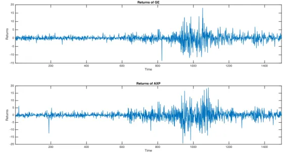
Since the main goal is to analyze volatility, the series are first transformed to log-return as 100 ·ln(pt/pt 1), where pt is the closed price. Thereafter the sample means of the

(30)

empirical analysis are the mean corrected log-returns. If not specified, we will use returns to refer to mean corrected log returns in the following analysis. Figure 5.1 depicts the returns. The first impression is that during some periods, both returns have fluctuated heavily. 200 400 600 800 1000 1200 1400 Time -15 -10 -5 0 5 10 15 20 Returns Returns of GE 200 400 600 800 1000 1200 1400 Time -20 -15 -10 -5 0 5 10 15 20 Returns Returns of AXP

Figure 5.1: The GE and AXP returns

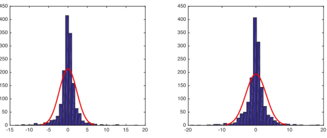
Figure 5.2 shows the histogram of both equities and the estimated normal distribution density function. We can conclude that the distribution of the returns does not follow a Gaussian distribution because there are large gaps between the fitted density function and the histogram. Table 5.1 presents descriptive statistics of the returns. Due to the mean correction, the means of both returns are zero and therefore not shown in the table. For both returns, the skewness is positive which suggests that the right tail of the distribution is fatter than the left tail. In addition, the kurtosis of both returns are greater than three which similarity to the histogram points to leptokurtic distributions with fat tails. Finally, the p-values of the Jarque-Bera test are almost zero indicating non-normality of both returns.

(31)

-15 -10 -5 0 5 10 15 20 0 50 100 150 200 250 300 350 400 450 -20 -10 0 10 20 0 50 100 150 200 250 300 350 400 450

Figure 5.2: Histogram of the GE and AXP returns and the estimated density function of normal distri-bution

Descriptive Statistics GE Returns AXP Returns

St.Dev 2.27 3.00 Median 0.02 0.01 Min -13.63 -19.34 Max 18.04 18.78 Skewness 0.02 0.08 Kurtosis 9.77 8.03

Jarque-Bera p-value = 0.001 p-value = 0.001

Table 5.1: Descriptive Statistics of the GE and AXP Returns

5.1.1 GARCH E

ﬀ

ects

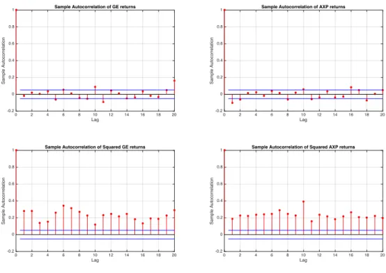
Figure 5.1 shows the typical volatility clustering observed in stock returns. In absolute value, large returns tend to be followed by large returns and small returns tend to be followed by small returns. Using the sample autocorrelation functions (ACF) of the series and their squares, Figure 5.3 shows that another typical feature of stocks returns holds true for the GE and AXP series. In the ACF plots, the vertical lines show the sample

(32)

autocorrelations at diﬀerent lags and the horizontal lines show the 0.05 critical bound. Sample autocorrelations within the critical bounds supports lack of correlation for both series. Figure 5.3 shows lack of autocorrelation in returns but strong autocorrelation in squared returns. This is a feature that can be captured by a GARCH model.

0 2 4 6 8 10 12 14 16 18 20 Lag -0.2 0 0.2 0.4 0.6 0.8 1 Sample Autocorrelation

Sample Autocorrelation of GE returns

Sample Autocorrelation of AXP returns

Sample Autocorrelation of Squared GE returns

Sample Autocorrelation of Squared AXP returns

Figure 5.3: Autocorrelation functions of the GE and AXP returns: sample ACF of GE returns (above left), sample ACF of squared GE returns (below left), sample ACF of AXP returns (above right) and sample ACF of squared AXP returns (below right).

5.1.2 Examining Potential Asymmetry

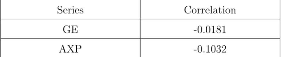
Before applying GARCH models, it is of interest to examine potential leverage eﬀects, the existence of which would suggest the use of an asymmetric GARCH model in analysis. We

(33)

use the simple idea of Zivot [25] and examine the sample correlation between the squared return y2

t and the lagged returnyt 1. A non-zero value of this suggests potential leverage

eﬀects exist in the time series.

Series Correlation

GE -0.0181

AXP -0.1032

Table 5.2: Correlation betweeny2

t andyt 1

The estimates obtained for the GE returns and AXP returns are -0.0181 and -0.1032 respectively. Thus, no strong indication about the leverage eﬀect is obtained, which can be testified by the estimated parameters in the asymmetric GARCH models in the estimation part.

5.1.3 Correlation between the returns

By comparing the time series graphs of the two returns, we find that they exhibit simi-larities. For example, between observations 1 and 600, both volatility are small whereas between observations 800 and 1200 both of them are much lager. This supports the idea that the returns are dependent. Figure 5.4, (a), (b) and (c) shows scatterplots of the re-turns. The plot in (a) shows that the two returns are contemporancously correlated while they are uncorrelated one of them is lagged with on day. This demonstrates the rationality to apply the multivariate models introduced in the previous part chapters.

(34)

-15 -10 -5 0 5 10 15 20 GE returns -20 -15 -10 -5 0 5 10 15 20 AXP returns -15 -10 -5 0 5 10 15 20 1 Lagged GE returns -20 -15 -10 -5 0 5 10 15 20 AXP returns -15 -10 -5 0 5 10 15 20 GE returns -20 -15 -10 -5 0 5 10 15 20

1 Lagged AXP returns

Figure 5.4: Scatter plot of GE and AXP: (a). The scatter plot of the GE and AXP returns (above left). (b). The scatter plot of the 1-lagged return of GE and the AXP return (above right). (c). The scatter plot of the 1-lagged return of AXP and the GE return (below left).

5.2 Estimation

In this section, the models introduced in Chapter 3 are applied to the observed data. Initially, we employ parsimonious GARCH models, i.e., GARCH(1,1), QGARCH(1,1) and GJR-GARCH(1,1). After that we consider multivariate models starting with the static models, i.e., the CCC-GARCH model and its special case, independent univariate GARCH models. Thereafter, we focus on the dynamic correlation models, i.e., DCC-GARCH models and ADCC-DCC-GARCH models.

(35)

Metropolis-within-Gibbs algorithm discussed in section 4.2.3. As we have no information on the prior, we follow the approach mentioned in 4.2.1 and adopt independent uninformative priors and implementing the algorithm on the likelihood function.

Meanwhile, we also need to impose parameter restrictions on the sample procedure to guarantee the employed models are stationary and the conditional variances are positive as well as the conditional correlation matrices are positive definite. Table 5.3, Table 5.4 and Table 5.5 summarize the conditions for each in the each models. To understand

Model Parameter restrictions

GARCH(1,1) ↵+ <1

QGARCH(1,1) ↵+ <1

GJR-GARCH(1,1) ↵+ ₂ + <1

Table 5.3: Restrictions for stationarity [3], [20], [16]

Model Parameter restrictions

GARCH(1,1) !,↵, >0

QGARCH(1,1) !,↵, >0, 4↵! 2 ₀

GJR-GARCH(1,1) !,↵, >0

Table 5.4: Restrictions for positive conditional variance (See Chapter 2)

CCC 1<⇢ij <1

DCC a+b _1 ,a, b >0

ADCC a+b+ g <1, a, b, g >0

(36)

and use these conditions, we select the CCC-GARCH(1,1) model as an example. Firstly, to satisfy the stationary condition and positive conditional variance , it is essential to ensure ↵+ <1 and !,↵, >0 for both of the two GARCH(1,1) models. Secondly, to

ensure that the correlation matrix is positive definite, we need 1<⇢12 <1.

Finally, we generate sample of size 5,000 for the parameter vector ✓ with burn-in the

first 1000 samples. As mentioned in the section 4.2.2, we adopt the expectation of the posterior samples as an estimate of ✓. However, when we shall compare the performance

of diﬀerent models with Bayesian Information Criterion (BIC) [19] we need the maximum likelihood estimate and for this purpose we use to the mode of the posterior samples which should provide a close approximation for the ML estimation [7].

5.2.1 Estimation of Static Correlation Model

After the preliminary analysis, now we have a multivariate return series yt = (y1,t, y2,t)0,

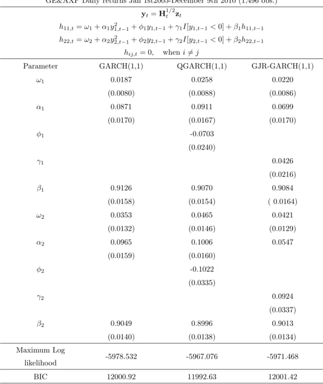
t = 1, . . . , T, in which y1,t is the return of GE andy2,t is the return of AXP. Table 5.6 and

Table 5.7 presents parameter estimates for the independent univariate GARCH model and the CCC-GARCH model respectively (Numbers in parentheses below estimates are standard errors obtained as standard deviations from the MWG samples). The estimates of i are around 0.9 in all models implying strong conditional heteroskedasticity in both

returns. Furthermore, the negative estimates of i in the QGARCH model and positive

estimates of iin the GJR-GARCH model suggest to leverage eﬀects. The leverage eﬀects

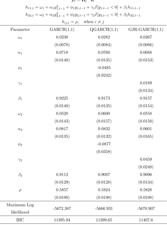
are not very strong in some cases, however, and this is particularly the case for the first component of the CCC-GJR-GARCH model in Table 5.7. In the CCC-GARCH model, the positive estimated of the correlation coeﬃcient ⇢ implies that the two stocks are

(37)

GE&AXP Daily returns Jan 1st2005-December 9th 2010 (1,496 obs.) yt=H1/2t zt h11,t=!1+↵1y2 1,t 1+ 1y1,t 1+ 1I[y1,t 1<0] + 1h11,t 1 h22,t=!2+↵2y2 2,t 1+ 2y2,t 1+ 2I[y2,t 1<0] + 2h22,t 1 hij,t= 0, wheni₆=j

Parameter GARCH(1,1) QGARCH(1,1) GJR-GARCH(1,1)

!1 0.0187 0.0258 0.0220 (0.0080) (0.0088) (0.0086) ↵1 0.0871 0.0911 0.0699 (0.0170) (0.0167) (0.0170) 1 -0.0703 (0.0240) 1 0.0426 (0.0216) 1 0.9126 0.9070 0.9084 (0.0158) (0.0154) ( 0.0164) !2 0.0353 0.0465 0.0421 (0.0132) (0.0146) (0.0129) ↵2 0.0965 0.1006 0.0547 (0.0159) (0.0160) 2 -0.1022 (0.0335) 2 0.0924 (0.0337) 2 0.9049 0.8996 0.9013 (0.0140) (0.0138) (0.0134) Maximum Log likelihood -5978.532 -5967.076 -5971.468 BIC 12000.92 11992.63 12001.42

(38)

GE&AXP Daily returns Jan 1st2005-December 9th 2010 (1,496 obs.) yt=H1/2t zt h11,t=!1+↵1y2 1,t 1+ 1y1,t 1+ 1I[y1,t 1<0] + 1h11,t 1 h22,t=!2+↵2y2 2,t 1+ 2y2,t 1+ 2I[y2,t 1<0] + 2h22,t 1 hij,t=⇢, wheni₆=j

!1 0.0230 0.0282 0.0267 (0.0078) (0.0084) (0.0086) ↵1 0.0718 0.0760 0.0688 (0.0140) (0.0135) (0.0153) 1 -0.0485 (0.0242) 1 0.0189 (0.0134) 1 0.9225 0.9173 0.9157 (0.0140) (0.0135) (0.0154) !2 0.0520 0.0600 0.0558 (0.0143) (0.0157) (0.0150) ↵2 0.0817 0.0832 0.0601 (0.0135) (0.0132) (0.0165) 2 -0.0877 (0.0358) 2 0.0459 (0.0248) 2 0.9112 0.9087 0.9096 (0.0129) (0.0128) (0.0134) ⇢ 0.5857 0.5824 0.5828 (0.0198) (0.0198) (0.0198) Maximum Log likelihood -5672.387 -5666.931 -5670.907 BIC 11395.94 11399.65 11407.6

(39)

Below the estimates, the maximum value of the log likelihood function and BIC are given for each model (see the discussion at the end of the preceding section), these will be discussed when comparing all estimated models in section 5.4.

5.2.2 Estimation of Dynamic Correlation Model

To estimate the parameters of DCC-GARCH and ADCC-GARCH models, we employe the two-step method proposed by Engle [8]. The first step is to estimate a univariate GARCH model and use the resulting estimates in the second step to estimate the remain-ing parameters. Specifically, we first implement the MWG algorithm on the univariate GARCH model, then the first component on the right hand side of (4.6), logLv(Y|')

becomes a fixed constant after the first step. Once we have estimated the parameters for the univariate GARCH models, Engle [8] suggests that we can use 1

n

PT

t=1✏t✏0tto estimate

¯

Q and _n1 PT_t₌₁ntn0t to estimate N¯ (see Definition 3.2.1 and Definition 3.3.1). Therefore,

it suﬃces to run the MWG algorithm on the second component in (4.6), logLc(Y| ).

The first step estimates we use are those given in Table 5.6. Those estimates are used in computing the the log-likelihood function (4.7), which is applied to DCC-GARCH models and ADCC-GARCH models estimation. Table (5.8) and Table (5.9) present the estima-tion results obtained in this way (Numbers in parentheses below estimates are standard errors obtained as standard deviations from the MWG samples).

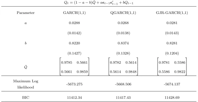
In both dynamic conditional correlation models, the estimates of b are around 0.8 while the estimates of a are close to 0.02. This shows that the Qt matrix is relative stable as it

depends much on its previous state and fluctuation caused by the standardised residual

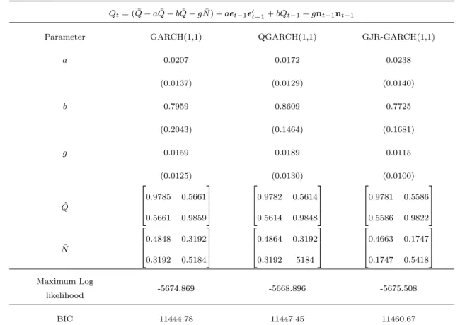
is small. In the ADCC-GARCH(1,1) model, the estimates of g are exist and around

0.02, which supports the existence of asymmetric eﬀects caused by negative and positive returns, but these eﬀects are not strong.

(40)

GE&AXP Daily returns Jan 1st 2005-December 9th 2010 (1,496 obs.)

Qt= (1 a b) ¯Q+a✏t 1✏0t 1+bQt 1

a 0.0288 0.0268 0.0281 (0.0142) (0.0138) (0.0143) b 0.8220 0.8374 0.8281 (0.1427) (0.1328) (0.1204) ¯ Q 2 6 6 4 0.9785 0.5661 0.5661 0.9859 3 7 7 5 2 6 6 4 0.9782 0.5614 0.5614 0.9848 3 7 7 5 2 6 6 4 0.9781 0.5586 0.5586 0.9822 3 7 7 5 Maximum Log likelihood -5673.275 -5668.506 -5674.137 BIC 11412.34 11417.43 11428.69

Table 5.8: Parameter estimates for DCC-GARCH models based on the univariate models in Table 5.6

5.3 Model Diagnostics

After having estimated the parameters of a model, we need to check the adequacy of the model. Regarding this, we show in Appendix A.4 autocorrelation functions of empirical counterpart of the standardized residuals obtained as

ˆ

zt=ytHˆt1/2 (5.1)

whereytis the vector of returns andHˆtis the conditional covariance matrix based on the

estimated models. In this case autocorrelations of the squared residuals are of interest and a model is deemed adequate if autocorrelations of squared standardised residuals are within the critical bound similar to those in Figure 5.3. In the ACF plot in Appendix A.4, they show no autocorrelation in the squared returns, i.e, no inadequacies in the estimated models.

(41)

GE&AXP Daily returns Jan 1st2 005-December 9th 2010 (1,496 obs.)

Qt= ( ¯Q aQ¯ bQ¯ gN¯) +a✏t 1✏0t 1+bQt 1+gnt 1nt 1

a 0.0207 0.0172 0.0238 (0.0137) (0.0129) (0.0140) b 0.7959 0.8609 0.7725 (0.2043) (0.1464) (0.1681) g 0.0159 0.0189 0.0115 (0.0125) (0.0130) (0.0100) ˆ Q 2 6 6 4 0.9785 0.5661 0.5661 0.9859 3 7 7 5 2 6 6 4 0.9782 0.5614 0.5614 0.9848 3 7 7 5 2 6 6 4 0.9781 0.5586 0.5586 0.9822 3 7 7 5 ˆ N 2 6 6 4 0.4848 0.3192 0.3192 0.5184 3 7 7 5 2 6 6 4 0.4864 0.3192 0.3192 5184 3 7 7 5 2 6 6 4 0.4663 0.1747 0.1747 0.5418 3 7 7 5 Maximum Log likelihood -5674.869 -5668.896 -5675.508 BIC 11444.78 11447.45 11460.67

Table 5.9: Parameter estimates for ADCC-GARCH models based on the univariate models in Table 5.6

5.4 Model Performance Comparison

In this section, we compare the performance of the estimated models using two criteria: the maximum value of the log likelihood function and the Bayesian Information Criterion (BIC).

By the definition, the maximum value of the likelihood function _Lˆ _{measures how well}

a model fits the data in comparison with alternative models, a high value of the like-lihood function indicates goodness of fit. However, the maximized value of likelike-lihood function does not allow for the complexity of the model caused by increasing the

(42)

num-ber of parameters, that is overfitting. The second criterion adopted to investigate the model performance is BIC, where a penalty term is used to guard against using too many parameters. The BIC, developed by Gideon E. Schwarz [19], is defined by:

BIC= 2_·ln ˆL+k_·ln(n) (5.2)

where

• Lˆ is the maximised value of the likelihood function of the model.

• k is the number of free parameters estimated.

• n is the number of observations data.

Models with small values of BIC are recommended. In (5.2), k_·ln(n) is the introduced

penalty term which penalises using an excessive number of parameters in the model. Achieving a high value of the likelihood function by increasing the number of parameters may not result in a favourable model in terms of BIC because the value of the penalty term is also increased.

Referring to the value of likelihood function and BIC computed by the mode of the pos-terior samples, comparing the static correlation models in terms of the value of the maxi-mized likelihood function shows that the asymmetric GARCH(1,1) models are preferable to the symmetric GARCH(1,1) models. In addition, we can conclude that the CCC-GARCH models are better at capturing the series’ volatility than the corresponding inde-pendent univariate GARCH models. Regarding the BIC values of the univariate models, we notice that, in spite of having a higher likelihood value, the GJR-GARCH(1,1) model is not preferred by BIC in comparison to the GARCH(1,1) model which, however is out-performed by the QGARCH(1,1) model. As a group, the CCC-GARCH models still beat the univariate models according to BIC. Comparing the three CCC-GARCH models, the CCC-GARCH(1,1) turns out to be the best, followed by the CCC-QGARCH(1,1) model and CCC-GJR-GARCH(1,1) model.

(43)

Of the dynamic correlation models, the DCC-GARCH models beat the ADCC-GARCH models according to likelihood value as well as according to BIC. In each group, mod-els with the QGARCH(1,1) model used to describe the conditional variance are the best according to the likelihood value but the BIC suggests the more parsimonious DCC-GARCH(1,1) or ADCC-DCC-GARCH(1,1) model. From the definition of the DCC-GARCH and GARCH models, we know that DCC-GARCH models are nested in GARCH models so that according to maximised values of the likelihood function, ADCC-GARCH models should be preferred. A possible reason why this is not the case is that in the two-step estimation, _Q¯ _and _N¯ _{are not maximum likelihood estimates and bias exists.}

Finally, we discuss the performance across the static correlation models and dynamic cor-relation models. If we check the performance according to the maximum likelihood value, the CCC-QGARCH(1,1) model is selected. As the CCC-GARCH model is a special case of DCC-GARCH model, the DCC-GARCH MODEL would be preferred by the maximum likelihood value theoretically, but comparing all the CCC-GARCH models and DCC-GARCH models, we find that the maximum likelihood value chooses the CCC-DCC-GARCH model. This is another evidence to show that the two-step method is biased. As to the other criterion, BIC, it still recommends the CCC-GARCH(1,1) model. An interpretation is that correlation exists in the returns but a constant correlation specification is sufficient to capture it. In addition, the leverage effect exists but it is not strong and BIC insists that THE symmetric GARCH model is sufficient to describe the volatility in the two returns series.

(44)

Chapter 6 Application to computing Value at

Risk

In this section, we compare the performance of the estimated multivariate GARCH models in computing the in sample Value at Risk and forecasting out sample Value at Risk.

6.1 Application in estimating VaR

VaR, which is short for Value at Risk, is one of the most popular techniques used in risk management to estimate the worst expected loss at a given probability level. We define the VaR of a portfolio:

Definition 6.1.1. Let rt be a daily return at day t and ⌘ 2 (0,1]. Then the VaR is a

real number VaR⌘ such that:

(45)

where Pt 1(·) denotes the conditional probability given the available information at day

t 1.

If we have a single asset and the returns follows the definition rt=µ+ p

htztwith ht and

zt independent andzt⇠N(0,1), we can compute the VaR as follows

VaR⌘ =µ+

p

htzt,⌘ (6.2)

where zt,⌘ is the ⌘-quantile of the distribution of zt.

The definition of VaR is usually given for a single index or a single asset. But in practice, it is often used for a portfolio of several assets. This can be done as follows: suppose we have n diﬀerent risky assets in a portfolio with a weight vector w = (w1, . . . , wn)0 and

assume these assets’ returns follow Definition 3.0.1 so thatrt=µ+Ht1/2zt, whereHtis the

conditional covariance matrix, zt⇠N(0,I)andztandHtindependent. Consequently, we

can derive the distribution of the portfolio by using the properties of multivariate normal distribution. Specifically, the portfolio w0rt follows a univariate normal distribution with

mean w0_µ_{and conditional variance} _w0_H

tw and Equation 6.2 can be rewritten as:

VaR⌘ =w0µ+zt,⌘

p

w0_H

tw (6.3)

Thus, the VaR also works as a risk measure of multivariate returns.

After the calculation of VaR, there are many tests which can be used to compare the performance of comparing models in terms of VaR. We use the test of Kupiec [15] , which compare the relative number of violations in VaR with the chosen probability level ⌘.

Here a violation means that the daily return is less than the VaR value of the day. If the number of VaR’s computed isN and the number of violations is x, it is reasonable to treat x as a Boernoulli distributed random variable with parameter ⌘. The idea of the Kupiec

test is to compare the observed violation rate ⌘ˆ=x/N with the chosen probability level

(46)

from its theoretical counterpart ⌘. Kupiec built the test on the likelihood ratio:

LR= 2 ln⌘ˆ

x₍₁ _⌘_ˆ₎N x

⌘x₍₁ _⌘₎N x (6.4)

In the case of a correctly specified model, test statistic LR is asymptotically chi-square distributed with one degree of freedom and large values of the test statistic are critical. Now we are ready to discuss how we apply the Kupiec test. We select⌘= 0.95and assume

that both stocks GE and AXP are held in the portfolio with equal 50% shares. As we subtract the mean of returns in the preliminary analysis, µ= (0, . . . ,0)0 _{and the returns}

are assumed to follow a conditional normal distribution with mean zero and covariance matrix is Ht, hence Equation (6.3) can be simplified as:

VaR0.95= 1.65

p

w0_H

tw (6.5)

where the theoretical conditional covariance matrixHtis replaced by an estimate obtained

from the estimated model.

In the following two sections, we first apply the Kupiec test within the sample period and then out of the sample period. We use the 5% significant level so that the critical value of the chi-square distribution with one degree freedom is 3.84. Thus, a value of the test statistic greater than 3.84 casts doubt on the adequacy of the model.

6.1.1 In-sample test

In the in-sample test, we will compute the conditional covariance matrix Htand compute

the VaR0.95according to Equation (6.5). The figures in Appendix A.5 show time series the

VaR0.95 computed with diﬀerent models and the composed returns of both stocks within

the sample data.

(47)

Models Relative number of violations LR Value GARCH(1,1) 0.088 36.8333 QGARCH(1,1) 0.086 34.4582 GJR-GARCH(1,1) 0.087 35.6373 DCC-GARCH(1,1) 0.046 0.4693 DCC-QGARCH(1,1) 0.046 0.4693 DCC-GJR-GARCH(1,1) 0.045 0.6513 ADCC-GARCH(1,1) 0.053 0.4693 ADCC-QGARCH(1,1) 0.053 0.4693 ADCC-GJR-GARCH(1,1) 0.045 0.8642 CCC-GARCH(1,1) 0.047 0.1960 CCC-QGARCH(1,1) 0.045 0.6513 CCC-GJR-GARCH(1,1) 0.044 1.1083

Table 6.1: Results of the in-sample Kupiec test with critical value of the LR test statistic is 3.84

The results show that the univariate models perform much worse than the multivariate models. The diﬀerence in the LR value among the univariate models is rather small and the same is true for the multivariate models. The results indicates that allowing for the correlation between the two returns is advantageous.

6.1.2 Out-sample test

In this section, we implement out-of-sample Kupiec test by using the returns of GE and AXP from 9th December 2010 to 9th December 2014, with totally 1006 daily log returns. In computing the conditional covariance matrix Ht to estimate the VaR, the same

(48)

esti-Models Relative number of violations LR Value GARCH(1,1) 0.060 2.2502 QGARCH(1,1) 0.059 1.5043 GJR-GARCH(1,1) 0.063 3.1359 DCC-GARCH(1,1) 0.033 7.0925 DCC-QGARCH(1,1) 0.032 8.0030 DCC-GJR-GARCH(1,1) 0.033 7.0925 ADCC-GARCH(1,1) 0.034 6.2446 ADCC-QGARCH(1,1) 0.031 8.7981 ADCC-GJR-GARCH(1,1) 0.033 7.0925 CCC-GARCH(1,1) 0.029 11.1301 CCC-QGARCH(1,1) 0.028 12.3115 CCC-GJR-GARCH(1,1) 0.028 12.3115

Table 6.2: Results of the out-sample Kupiec test with critical value of the LR test statistic is 3.84

mates from the previous in-sample data are used for all models without update. Figures in Appendix A.5 present the VaRs based on one day ahead forecasts and returns, whereas Table 6.2 displays the test results. The out-of-sample results in Table 6.2 are completely contrary to the in-sample results in Table 6.1 in that the out-of-sample Kupiec test clearly rejects all multivariate models. A possible reason is that without updating estimates, the multivariate GARCH models lose accuracy in the forecasting of the conditional covariance matrix Ht when the prediction period is too long. To examine this assumption, we do

(49)

Models Relative number of violations LR Value GARCH(1,1) 0.070 2.2590 QGARCH(1,1) 0.067 1.5955 GJR-GARCH(1,1) 0.070 2.2590 DCC-GARCH(1,1) 0.033 1.9779 DCC-QGARCH(1,1) 0.033 1.9779 DCC-GJR-GARCH(1,1) 0.033 1.9779 ADCC-GARCH(1,1) 0.037 1.2325 ADCC-QGARCH(1,1) 0.033 1.9779 ADCC-GJR-GARCH(1,1) 0.033 1.9779 CCC-GARCH(1,1) 0.033 1.9779 CCC-QGARCH(1,1) 0.037 1.2325 CCC-GJR-GARCH(1,1) 0.037 1.2325

Table 6.3: Results of the out-sample Kupiec test with critical value of the LR test statistic is 3.84 on the first 300 observations

Under 5% significant level, the multivariate models are still adequate in describing and forecasting the VaR. The diﬀerent results in Table 6.2 and Table 6.3 suggest that when the multivariate conditional correlation models are used, the volatility forecast period should be appropriate to ensure accuracy and if it is permitted, one should update the parameters estimates once the new data comes available.

(50)

Chapter 7 Conclusion and Future Work

In the thesis, we studied multivariate conditional correlation GARCH models, including the CCC-GARCH, DCC-GARCH and ADCC-GARCH models. In constructing the con-ditional variances, three types of univariate GARCH models were employed: GARCH, the QGARCH and GJR-GARCH model. These models were applied to the daily returns of the General Electric Company and American Express Company.

In the parameter estimation of dynamic correlation models, we adopted the two steps method suggested by Engle [8]. Instead of the regular maximum likelihood estimation, we implemented a Markov Chain Monte Carlo algorithm, Metropolis within Gibbs algo-rithm.

After estimating the parameters of each model in the empirical application, we first stud-ied the adequacy of the models and found that all of them are capable of describing the heteroskedasticity in the data. We also compared goodness of fit of the models by max-imum value of the likelihood function and Bayesian Information Criterion. They gave diﬀerent result. The likelihood function suggested the CCC-QGARCH(1,1) model while BIC favourited the CCC-GARCH(1,1) model. Finally, all the models were applied to

(51)

compute VaR and the Kupiec test was used to check the performance of the models. The in-sample test showed that the univariate models are inadequate in computing VaR. According to the out-of-sample test, all the models are able to forecast and estimate the VaR, but the out-of-sample period should be short for the conditional correlation GARCH models.

There are two points that can be improved in future work.

1. In the estimation of the DCC-GARCH model, we always estimated the parameter matrices _Q¯ _by 1

n

PT

t=1✏t✏0t. An idea is whether the estimated correlation matrix R

from the CCC-GARCH model can be used instead. In a numerical experiment, the resulting two-step estimate performed better than the one suggested by Engle [8], but it lacks the theoretical support, which may be developed in future work. 2. Instead of the two-step method, one can estimate the parameters of the

DCC-GARCH or ADCC-DCC-GARCH models by implementing a MCMC algorithm on the likelihood function as a whole to eliminate the error caused by two step methods. The Metropolis within Gibbs algorithm has been tried but the speed of convergence turned out to be slow, so that some other algorithm need to be employed.

(52)

Appendix A

A.1 Metropolis Hasting algorithm

Algorithm 1: Metropolis Hasting algorithm

input : An initial value ✓(0) _{such that} _⇡₍_✓(0)₎_>₀ _{and the number of iterations}_N_.

Result: To have N enough target distribution samples to approximate the true value.

Initialization;

for i= 1 :N do current state ✓cur_;

sample a posterior ✓0_;

sample random variable ufrom standard uniform distribution;

if u < p = min{1,_⇡⇡₍_✓(✓cur0|y_|_y)·₎q_·(_q✓₍_✓cur0_|✓|cur✓0)₎} then

✓cur ₌_✓0_;

✓(i)₌_✓_;

end end

(53)

A.2 Gibbs sampling algorithm

Algorithm 2: Gibbs Sampling

Initialization;

✓cur _✓(0)_;

for i= 1 :N do

for j = 1 : d do

draw a new value for thejth component ✓cur

j of ✓cur from the posterior full

conditional⇡_✓j|✓ j(✓j|✓ cur j ) end ✓i+1 _✓cur_; end

(54)

A.3 Metropolis Within Gibbs sampling algorithm

Algorithm 3: Metropolis Within Gibbs sampling algorithm

Initialization;

✓cur _✓(0)_;

for i= 1 :N do

for j = 1 : d do current state ✓cur

j ;

sample a posterior ✓0

j;

sample random variableu from standard uniform distribution;

if u < p= min_{1, ⇡(✓0j|y)·q(✓cur|✓0j) ⇡(✓cur j |y)·q(✓j0|✓curj )} then ✓cur j =✓0j; ✓(_ji) =✓cur j ; end end ✓i+1 _✓cur_; end

(55)

A.4 Sample ACF of standardised residuals

Sample Autocorrelation of Squared Standardized Residuals of GE returns

(a) Sample ACF of GE returns residuals stan-dardised by univariate GARCH(1,1)

Sample Autocorrelation of Squared Standardized Residuals of AXP returns

(b) Sample ACF of AXP returns residuals stan-dardised by univariate GARCH(1,1)

(a) Sample ACF of GE returns residuals stan-dardised by univariate QGARCH(1,1)

(b) Sample ACF of AXP returns residuals stan-dardised by univariate QGARCH(1,1)

(a) Sample ACF of GE returns residuals stan-dardised by univariate GJR-GARCH(1,1)

(b) Sample ACF of AXP returns residuals stan-dardised by univariate GJR-GARCH(1,1)

(56)

(a) Sample ACF of GE returns residuals stan-dardised by CCC-GARCH(1,1) 0 2 4 6 8 10 12 14 16 18 20 Lag -0.2 0 0.2 0.4 0.6 0.8 1 Sample Autocorrelation

(b) Sample ACF of AXP returns residuals stan-dardised by CCC-GARCH(1,1) 0 2 4 6 8 10 12 14 16 18 20 Lag -0.2 0 0.2 0.4 0.6 0.8 1 Sample Autocorrelation

(a) Sample ACF of GE returns residuals stan-dardised by CCC-QGARCH(1,1) 0 2 4 6 8 10 12 14 16 18 20 Lag -0.2 0 0.2 0.4 0.6 0.8 1 Sample Autocorrelation

(b) Sample ACF of AXP returns residuals stan-dardised by CCC-QGARCH(1,1) 0 2 4 6 8 10 12 14 16 18 20 Lag -0.2 0 0.2 0.4 0.6 0.8 1 Sample Autocorrelation

(a) Sample ACF of GE returns residuals stan-dardised by CCC-GJR-GARCH(1,1) 0 2 4 6 8 10 12 14 16 18 20 Lag -0.2 0 0.2 0.4 0.6 0.8 1 Sample Autocorrelation

(b) Sample ACF of AXP returns residuals stan-dardised by CCC-GJR-GARCH(1,1)