ventions in the Pediatric Intensive Care Unit: A Demonstration of Longitudinal Targeted Maximum Likelihood Estimation. American journal of epidemiology, 186 (12). pp. 1370-1379. ISSN 0002-9262 DOI: https://doi.org/10.1093/aje/kwx213
Downloaded from: http://researchonline.lshtm.ac.uk/4645978/
DOI:10.1093/aje/kwx213
Usage Guidelines
Please refer to usage guidelines at http://researchonline.lshtm.ac.uk/policies.html or alterna-tively [email protected].
American Journal of Epidemiology
© The Author(s) 2017. Published by Oxford University Press on behalf of the Johns Hopkins Bloomberg School of Public Health. This is an Open Access article distributed under the terms of the Creative Commons Attribution License (http://creativecommons. org/licenses/by/4.0), which permits unrestricted reuse, distribution, and reproduction in any medium, provided the original work is properly cited.
Vol. 186, No. 12 DOI: 10.1093/aje/kwx213 Advance Access publication: June 24, 2017
Practice of Epidemiology
Estimating the Comparative Effectiveness of Feeding Interventions in the
Pediatric Intensive Care Unit: A Demonstration of Longitudinal Targeted
Maximum Likelihood Estimation
Noémi Kreif*, Linh Tran, Richard Grieve, Bianca De Stavola, Robert C. Tasker, and Maya Petersen
*Correspondence to Dr. Noémi Kreif, Centre for Health Economics, University of York, Heslington, York YO10 5DD, United Kingdom (e-mail: [email protected]).
Initially submitted June 2, 2016; accepted for publication March 31, 2017.
Longitudinal data sources offer new opportunities for the evaluation of sequential interventions. To adjust for time-dependent confounding in these settings, longitudinal targeted maximum likelihood based estimation (TMLE), a dou-bly robust method that can be coupled with machine learning, has been proposed. This paper provides a tutorial in applying longitudinal TMLE, in contrast to inverse probability of treatment weighting and g-computation based on iter-ative conditional expectations. We apply these methods to estimate the causal effect of nutritional interventions on clinical outcomes among critically ill children in a United Kingdom study (Control of Hyperglycemia in Paediatric Inten-sive Care, 2008–2011). We estimate the probability of a child’s being discharged alive from the pediatric intensive care unit by a given day, under a range of static and dynamic feeding regimes. Wefind that before adjustment, pa-tients who follow the static regime“never feed”are discharged by the end of thefifth day with a probability of 0.88 (95% confidence interval: 0.87, 0.90), while for the patients who follow the regime“feed from day 3,”the probability of discharge is 0.64 (95% confidence interval: 0.62, 0.66). After adjustment for time-dependent confounding, most of this difference disappears, and the statistical methods produce similar results. TMLE offers aflexible estimation approach; hence, we provide practical guidance on implementation to encourage its wider use.
causal inference; epidemiologic methods; longitudinal targeted maximum likelihood estimation; machine learning; Super Learner; time-dependent confounding
Abbreviations: CHiP, Control of Hyperglycemia in Paediatric Intensive Care; CI, confidence interval; IPTW, inverse probability of treatment weighting; PICU, pediatric intensive care unit; RACHS-1, Risk Adjustment for Congenital Heart Surgery; TMLE, targeted maximum likelihood estimation.
Large observational databases such as electronic health rec-ords are increasingly being used to answer questions of com-parative effectiveness. The longitudinal structure of these data sets allows researchers to estimate the effects of interventions that change over time. Examples include the treatment of chronic diseases such as diabetes and hypertension, where deci-sions such as when to initiate a treatment, change the dose, or introduce a concomitant medication are repeatedly updated over time. For decision-makers to compare the consequences of alternative longitudinal interventions, it is essential to carefully define the strategies of interest (1). A static regime for time-varying interventions prespecifies the full sequence of interven-tions, irrespective of changing patient characteristics over time
(e.g.,“always treat”). Dynamic regimes, or individualized treat-ment rules, in contrast, define a set of rules as a function of time-varying patient characteristics (2–6). While sequentially randomized trials provide an ideal design for the evaluation of dynamic regimes (7,8), such trials are still relatively rare (9) and are impractical for many clinical and health policy ques-tions (10).
Where the only available data for estimating the treatment ef-fects of interest are from observational studies, statistical meth-ods are required to address both baseline and time-dependent confounding. The latter arises in longitudinal settings, when the uptake of treatment may depend on factors that influence the outcome and are also affected by earlier treatments. It is widely
recognized that standard regression analysis cannot deal with time-dependent confounding (2,11). While in the last few decades progress has been made in developing appro-priate statistical methods for addressing time-varying con-founding (see Daniel et al. (12) for a review), applications of these approaches have been confined to relatively few clinical areas, such as human immunodeficiency virus infection (13). Further methodological and applied research that demon-strates these approaches for handling time-varying con-founding in different contexts is required.
Inverse probability of treatment weighting (IPTW) (11,14), a simple and intuitive method for estimating the effect of time-varying treatments, results in unstable and biased estimates in the presence of data sparsity, even when weights are normal-ized and extreme weights are truncated (15). A commonly used alternative approach, parametric g-computation (2), requires parametric specification of multiple aspects of the data distribution, including models for the full conditional densities (or probability distributions) of the outcome and of the time-dependent confounders given the past. Similarly, structural nested mean models require a parametric model for the treatment effect, the“blip function”(16). A perennial con-cern with these approaches is that they are prone to model mis-specification, leading to biased estimates of treatment effects.
Targeted learning (17) has been proposed as a general approach to estimation of a range of causal parameters for causal inference problems with both time-constant and time-varying interventions (18–22). Targeted learning encompasses a semi-parametric, doubly robust estimation approach, targeted maxi-mum likelihood estimation (TMLE) (17) for single-time-point and longitudinal causal effects. TMLE combines estimates of the treatment and outcome mechanisms and provides a consis-tent estimator of the target parameter if either the treatment or the outcome mechanism is estimated consistently. If both are estimated consistently, TMLE is efficient (19). In order to reduce bias, achieve efficiency, and ensure accurate statistical inference, TMLE is often coupled with machine learning— particularly the Super Learner, a cross-validation-based estima-tor selection approach (23,24). (For a tutorial on single-time-point interventions, see, for example, Schuler and Rose (25).)
In this paper, we demonstrate the application of the longitudi-nal TMLE estimator based on iterative conditiolongitudi-nal expectations (21,26) and highlight how it is related to the IPTW (11) and g-computation (2,26) estimators. While prior studies demonstrat-ing the application of this estimator in longitudinal settdemonstrat-ings exist (22,26–30), few observational data applications have discussed the use of the estimator to study the effects of dynamic regimes or subject-responsive adaptive treatment strategies (31).
We apply IPTW, g-computation based on iterative condi-tional expectations, and longitudinal TMLE to an empirical study investigating an unanswered question of high relevance to clinical decision-makers: What is the optimal timing and quantity of caloric intake for critically ill children? We reana-lyze data from a clinical trial, the Control of Hyperglycemia in Paediatric Intensive Care (CHiP) Study (32), to estimate the effect of alternative treatment regimes on the probability of being discharged from the pediatric intensive care unit (PICU) by a given day, under a range of clinically relevant treatment regimes. We follow the general targeted estimation road map (33) to formulate the hypothetical regimes, define the causal
parameters of interest, and discuss how to identify, estimate, and interpret these parameters.
METHODS
Research question in the CHiP Study
An important objective of critical-care medicine is to pro-vide the appropriate level of nutritional support over the course of the patient’s hospital stay. In most critical-care settings, the preferred mode of nutritional support is the nasogastric (enteral) tube, which is often complemented with intravenous (parenteral) feeding. For adult patients admitted to critical-care units, evidence-based guidelines exist, and in a recent randomized controlled trial, McClave et al. (34) re-ported that starting nutritional support early after admission to the PICU favorably altered outcomes. For critically ill children, guidelines for nutritional support are limited by the lack of available evidence (35). While a recent randomized trial of nutritional support for children admitted to the PICU found that delaying parenteral nutrition led to favorable clinical out-comes (36), there is no randomized trial evidence to address more complex but important questions, such as the optimal tim-ing and total quantity of nutritional support for children admit-ted to the PICU.
In recently publishedfindings from the CHiP Study, a ran-domized trial with 1,369 participants aged≤16 years (recruited between 2008 and 2011) undertaken at 13 research centers in the United Kingdom, Macrae et al. (32) found that tight glyce-mic control in critically ill children had no effect on the primary clinical outcome, the number of ventilator-free days. We under-took a secondary analysis of the CHiP data set to investigate the causal effect of different levels of nutritional support on a clini-cal outcome. We focused on the subgroup of children who were admitted to the PICU to undergo cardiac surgery and were younger than 3 years of age.
We followed the US National Academy of Medicine (for-merly Institute of Medicine) guidelines (37) in standardizing individual caloric intake by dividing the individual measures of daily intake by a target level specific to the patient’s sex, age, height, and weight. We defined a patient as“fed”on a given day if he or she received at least 20% of the individualized tar-get. The outcome of interest was being discharged alive from the PICU to other hospital wards by a given day.
The effect of a feeding strategy on a given day on the patient’s discharge status is subject to potential confounding from baseline characteristics, such as age, sex, weight, height, Risk Adjustment for Congenital Heart Surgery (RACHS-1) risk score (which ex-presses the severity of the child’s condition at admission (38)), and randomization arm (tight or standard glycemic control). Younger children and those with higher risk scores tend to be fed less aggressively and are also likely to stay longer in the PICU, potentially biasing the effect of feeding (as compared with no feeding) towards a seemingly protective effect. While all patients are mechanically ventilated at baseline, being taken off mechanical ventilation is a strong predictor of discharge in the next few days. Patients just taken off mechanical ventilation can, for safety reasons, be fed only by the parenteral (not the enteral) route, making it less likely that their caloric intake will reach the 20% threshold. Hence, a lack of adjustment for
mechanical ventilation status could make no feeding appear beneficial. Further time-varying potential confounders include renal replacement therapy, infection, and a vasoactive inotrope score (39).
Observed data structure
For each patient in the CHiP Study, the level of calorific intake (the treatment) was measured daily from study entry (randomization) until the relevant clinical outcome was re-corded (discharge from the PICU or death while in the PICU). We restricted the follow-up data used in this analysis to the first 7 days postrandomization, since the majority of patients were discharged from the PICU by this time point.
In our analysis, we denote time byt=0, ...,T+1, where + =
T 1 7is the end of follow-up. At each time point, the pa-tient’s feeding status is represented by the binary variableAt, while confounders are denoted by the multidimensional vari-ableZt. Thefirst measurement of the time-varying confounders and the vector of baseline confounders are jointly denoted by
Z0. Mechanical ventilation, renal replacement therapy,
infec-tion, and randomization arm are binary variables, while the RACHS-1 and vasoactive inotrope scores, weight, height, and age are continuous.
Mt andYt indicate whether, by the end of time periodt, a patient has died(Mt= ) 1 or has been discharged alive from the PICU(Yt= ) 1. We use overbars to denote histories; for example, treatment history is denoted by At = (A0, ...,At). We assume that the observed data arenindependent and identically distrib-uted copies ofO= (Z0,A0,Y M Z A1, 1, 1, 1, ...,AT,YT+1) ∼ Po, wherePois the true underlying distribution from which the data are drawn and where, for notational convenience, we assume that the values of variables after death or discharge are determin-istically equal to their last observed values. The ordering of the elements ofOrepresents their assumed causal ordering. (See Web Appendix 1, available athttps://academic.oup.com/aje, for the causal model.) For example, the baseline covariates(Z0) precede thefirst instance of feeding(A0), which precedes whether the patient is discharged by the end of thefirst day( )Y1.
We denote the history of the confounders, discharge status, and death with a single vectorLt= (Z Y Mt, t, t)that will be referred to as“covariates.”Death is treated as a competing event for PICU discharge: IfMt= 1, then any subsequent
=
′
Yt 0fort′ >t.
Formulating the interventions of interest
We consider 2 types of longitudinal interventions: static treat-ment regimes and dynamic treattreat-ment regimes. Let the vector
¯ = (a a a )
a 0, 1, ..., T denote a longitudinal feeding regime, defined up to the last period before the end of follow-up. The elements of this vector,at, define the feeding intervention, with static and dynamic regimes differing in howat is specified. For a static regime,atis a prespecified constant for eacht. For example, the static regime“never feed”setsatto 0 in eacht, resulting in the treatment regimea= ( 0, 0, ..., 0), while the static regime“feed from day 3”would be defined asa= ( 0, 0, 1, ..., 1).
For dynamic regimes, at is set by a decision rule. We definedtas a function that incorporates information available on a subject up to timet, such as some subset of the covariate
history, denotedV¯t. We used( )Vt to denote the vector of in-terventions required by regimedfrom time 0 to timet, given the realized covariate history. Here, we specify a dynamic treatment regime in which clinicians are required to feed a patient on each day that he or she is not mechanically venti-lated(Zt,1= ) 1.
Clinical guidelines may not require the intervention to start on thefirst day and could allow delaying the start of the intervention. For example, the regime“feed by the third day” leaves the treatment values to be random for 2 days and then requires feeding from day 3 onward. This regime is denoted bya¯2:T = (A0,A1, 1, ..., 1), whereA0andA1are the observed
levels of feeding on thefirst 2 days.
Throughout, we consider regimes that implicitly only assign a feeding intervention up to the time of discharge or death. Thus, a subject who followed a regime of interest up to death or discharge, according to our definition, would continue to follow this regime up to timeT+1. To simplify notation, in the sec-tions that follow, we refer to the counterfactual intervensec-tions generally asd= (d0, ...,dT) ∈D, whereDis the set of regimes of interest, and note that this notation includes static regimes as special cases of dynamic regimes.
Target causal parameter and identifying assumptions
The counterfactual discharge status at timetthat would have been observed under a given feeding regimedis denoted by Ytd. Our causal parameter of interest is the intervention-specific mean outcome, the expected discharge status by a selected time
⁎
t , under a given regimed, wheret⁎= 1, ...,T+1: ψd t,⁎=E Y[ td⁎].
ψd t,⁎can be interpreted as the counterfactual cumulative risk of discharge by dayt⁎if all subjects had followed a given
regime.
In order to identifyψd t,⁎from the observed data, the fol-lowing assumptions are required (2):
Thesequential randomization assumptionstates that, con-ditional on the observed treatment and confounder history, the potential outcome is independent of treatment status in each preceding time period,
⊥ | − = ( ¯−) ⁎
Ytd At L At, t 1 d Vt 1,
fort= 0, ...,t⁎−1, andd∈D. This assumption requires that a sufficiently rich set of confounders are measured, so that it can be assumed that conditional on observed covariates, and following the regime of interest, the feeding decision at time tis“at random.”
Thepositivity assumption requires that for each feeding regimed, in each periodtbefore thefinal time period of inter-estt⁎, patients must have a positive probability of following
that regime, conditional on having followed it up to that time point, for any combination of observed covariate history:
[A =d V( ) |L A− =d V( − )] >
Pr t t t, t 1 t 1 0,
fort = 0, ...,t⁎− 1.
Am J Epidemiol. 2017;186(12):1370–1379
Estimation: IPTW
In this section we describe the IPTW estimator, the g-computation estimator, and the longitudinal TMLE estimator. We focus on implementation of the estimators for interventions that start on thefirst day. For interventions with a delayed start, we provide small modifications of the estimators in Web Appendix 2. IPTW estimates the intervention-specific mean outcome of a treatment regime by reweighting the observed outcomes in the subset of the study sample who followed the regime (11). We denote the probability of a subject’s following a regime of inter-estdtat timet, given his/her covariate and treatment history, with
= [ = ( ) | − = ( −) ¯ ]
gt Pr At d Vt t At 1 d Vt 1,Lt ,
and the cumulative conditional probability of following regime dthrough timet⁎−1as
∏
= − = − ⁎ ⁎ g t g. t t t 0: 1 0 1The stabilized Horvitz-Thompson IPTW estimator (14,40) of the cumulative risk of discharge by periodt⁎under treatment
regimedis based on estimation of the following quantity:
[ × ( ¯ = ( ¯ )) ] [ ( ¯ = ( ¯ )) ] − − − − − − ⁎ ⁎ ⁎ ⁎ ⁎ ⁎ ⁎ E Y I A d V g E I A d V g / / , t t t t t t t 1 1 0: 1 1 1 0: 1
where I A( t⁎−1 =d V( t⁎−1)) indicates whether a patient has followed the treatment regimedup to one period before the final period of interest. Implementation is based on estimating gtfort= 0, ...,t⁎− 1, plugging in these estimates, and taking the empirical mean of the numerator and denominator.
Drawbacks of the IPTW estimator include reliance on con-sistent estimation of the treatment mechanism, as well as sus-ceptibility to violations and near violations of the positivity assumption, resulting in unstable estimates (see, for example, Petersen et al. (15)). In the next section, we describe the longi-tudinal TMLE estimator, a doubly robust estimator which can improve on the properties of the IPTW estimator by using information not only on the treatment mechanism but also on the outcome-confounder(s) relationship.
Estimation: longitudinal TMLE
The conditional expectation representation of the g-computation formula. Longitudinal TMLE (21) uses the iden-tifiability result established by the g-computation formula (2). In short, the g-computation formula expresses the intervention-specific mean outcome as a function of the conditional distribu-tions of the outcome and the time-varying confounders, given the past, among subjects who followed the regime of interest. For discrete-valued confounders, this can be written as follows:
∏
[ ] = ∑ [ | = ( ) = ] × ( = | = ( ) = ) − − − − = − − − − − ⁎ ⁎− ⁎ ⁎ ⁎ ⁎ ⁎ ⁎ E Y E Y A d v L l L l A d v L l , Pr , , td l t t t t t t t t t t t t t 1 1 1 1 0 1 1 1 1 1 t 1where the summation is taken over all possible valueslt⁎−1of
the confounder history. Intuitively, the g-computation formula estimates the conditional expectation of the outcome under the treatment regime of interest and averages these expectations over the intervened-on distribution of the confounders—that is, the distribution that the confounders would take under the treat-ment regime of interest. Parametric g-computation (2,41,42) estimates the components of this formula directly, and it makes strong parametric assumptions due to the need to specify condi-tional densities or probabilities for each of the time-varying con-founders (12,43).
The g-computation formula can be rewritten as a series of iterated conditional expectations of the observed outcome (26,44,45): [ ] = [… [ [ [ | = ( ) ] | = ( ) ] | = ( ) ]…] ( ) − − − − − − − − − ⁎ ⁎ ⁎ ⁎ ⁎ ⁎ ⁎ ⁎ ⁎ ⁎ ⁎ E Y E E E E Y A d V L A d V L A d V L , , , , 1 t d t t t t t t t t t t 1 1 1 2 2 2 3 3 3
where the innermost expectation is the conditional distribution of the outcome, given the full treatment and confounder history, evaluated at the treatment values that would have been assigned according to the intervention of interestd. The second innermost expectation marginalizes over the intervened-on history ofLt⁎−1,
the next one overLt⁎−2, and so on, until the last expectation is
taken over the empirical distribution of baseline confounders L0, whereM0= 0andY0= 0. Wefirst briefly review how to
obtain the target parameter using these iterative regressions and then describe how the longitudinal TMLE extends this approach.
Steps of g-computation using sequential regressions. Step 1: Regress the outcome on full treatment and confounder history. First the innermost expectation of equation 1 is estimated:
[ ⁎| ⁎− ⁎− = ( ⁎−)]
E Yt Lt 1,At 1 d Vt 1 .
We will refer to this quantity asQt⁎. This expectation can be estimated by regressing the outcome on past covariates and treatment variables—for example, using a logistic regression— and taking predictions at the treatment values corresponding to the intervention of interest.
Step 2: Take the previous predictions as the new outcome and regress on history up tot⁎− 2. The predictions from the previous step,Qt⁎are now taken as the new outcome and are re-gressed on confounders and treatment variables up to time period
−
⁎
t 2. As before, predictions are generated for treatment values required by the regimed, up to time periodt⁎−2. This expecta-tion,Qt⁎−1, corresponds to the second innermost expectation in
equation 1.Qt⁎−1is marginal over the intervened-on
distribu-tion of the time-varying confounderLt⁎−1but conditional on the
time-varying confounders up to time periodLt⁎−2.
Steps 3, 4, . . . to stept⁎: Iterate step 2. Step 3 takes the
predictions from step 2,Qt⁎−1, regresses them on the treatment
and confounder history up tot⁎−3, and then takes predictions as described above, stored asQt⁎−2. This step is iterated until
the last step, where the expectation is only conditional on the baseline covariates:
= [ | = ( )]
Q1 E Q L2 0,A0 d V0 .
Stept⁎+1: Average over the empirical distribution of the baseline covariates. By averagingQ1over the empirical
dis-tribution ofL0, the g-computation estimator for the
intervention-specific mean is obtained asQ0 =E Q[ 1].
EachQtcan be obtained using a regression—for example, a linear or logistic regression. This approach offers substantial ad-vantages over the parametric g-computation approach, by avoiding the need to estimate the conditional density of each time-varying confounder. However, estimating these iterative regressions well can be challenging, and the approach remains susceptible to bias due to misspecification. Bang and Robins (26) proposed a doubly robust and semiparametric efficient ver-sion of this sequential regresver-sion estimator based on including an additional,“clever”covariate that uses information from the treatment assignment mechanism. It has subsequently been sug-gested to move this clever covariate to a weight, an approach that improved performance in the face of practical positivity violations (46). The resulting estimator is doubly robust in the sense that if either the treatment mechanisms or the sequential regressions are estimated consistently, then the estimator is con-sistent. If both are estimated consistently, it is efficient in a semiparameteric model that makes assumptions, if any, only on the treatment mechanism (26). Van der Laan and Gruber (21) subseqently placed this estimator in the general TMLE frame-work. The general idea behind this TMLE is that it is a 2-step estimator: First the conditional expectation of the outcome is estimated, and then this estimate is updated using information from the treatment assignment mechanism, targeted in a way that it reduces bias for the parameter of interest. Longitudinal TMLE performs the update step at each stage of the sequential regressions, as we summarize below.
The update step of the TMLE estimator. Qt⁎ is defined and estimated as in step 1 of the g-computation approach. This initial estimate is then updated by perturbing the initial fitQt⁎using a parametric submodel, defined as
(Q⁎(ε )) =⁎ (Q⁎) + ε⁎
logit t t logit t t.
1
We estimateεt⁎ byfitting a logistic regression ofY⁎ t on the intercept, using the prior predicted value ofQt⁎as an offset, and weights corresponding toI A( ¯t⁎−1=d V( ¯t⁎−1))/g0:t⁎−1, an
indicator of whether a subject has followed the regime of inter-est up to the previous time period divided by the predicted probability of having done so. The estimatedεt⁎is then used to update the initial estimate, which is stored asQt1⁎, and will be used as the new outcome for the next iteration.
This update is performed after each step of the sequential re-gressions, described for the g-computation estimator. The regres-sion and update steps are iterated until the last step, in which the updated expectationQ11is only conditional on the baseline co-variates. Analogous with the last step of the g-computation estimator, the TMLE estimator for the intervention-specific mean is obtained asQ01=E Q[ 11].
The consistency of the estimator relies on consistent estima-tion of either the treatment mechanism or the iterated condiestima-tional regressions, while its efficiency relies on consistent estimation of both. In practice, often both components are expected to be
misspecified whenfixed, parametric models such as logistic regressions are used. Machine learning or data-adaptive ap-proaches are thus advocated for estimation of both (19). We use the Super Learner (47), a machine learning algorithm that uses cross-validation tofind the optimal weighted convex combination of multiple candidate prediction algorithms, for estimating both the treatment assignment mechanism and the sequential regressions (see Web Appendix 3 for more details).
Implementation
We implement the IPTW, g-computation, and TMLE estima-tors described above to estimate the cumulative probability of PICU discharge by the end of days 1–7, under a range of prespe-cified static treatment regimes (“never feed,” “feed from day 1, 2, 3, . . .7”), static regimes over limited time periods (“feed by day 2, 3, . . .7”), and the dynamic regime“feed when off ventilation.” We use the Super Learner to estimate the treatment assignment mechanism and the sequential regressions, and we use these models to construct the 3 estimators. Among the Super Learner candidates, we include an intercept model, a main-terms model, a logistic regression model with all possible 2-way interactions in the linear predictor, a stepwise logistic regression model, generalized additive models (48), a Bayesian generalized linear model with main terms in the linear predictor (49), a LASSO model (50), a boosting algorithm (51), and a neural networks algorithm (52). We specify 10-fold cross-validation (47). Wefit separate models for the treatment assignment mechanism for each period, while assuming that treatment decisions are infl u-enced only by treatment and confounder values in the 2 most recent periods. The regressions carried out to obtain the con-ditional probability of treatment and the iterative regressions and the update steps of the TMLE are only run among those children who remain alive and not discharged. We contrast these estimates with“naive”estimates, taken as the simple proportion of discharge status among those who follow a given regime.
The 95% confidence intervals are based on an estimate of the empirical influence function (53,54) of the IPTW and TMLE estimators. For the g-computation estimator, no infl uence-function-based approach for inference is readily available, and the point estimates are reported without 95% confidence inter-vals. While the nonparametric bootstrap represents an alterna-tive approach to variance estimation, when Super Learner is used to conduct the sequential regressions without subsequent targeting, bootstrapping can impose a substantial computational burden while still failing to provide valid inference. The avail-ability of an influence-curve-based variance estimator compati-ble with machine learning approaches is thus an additional attractive feature of TMLE. The methods are implemented using the package“ltmle”in R, version 0.9-9 (R Foundation for Statistical Computing, Vienna, Austria) (55,56), which incor-porates the Super Learner R package (57). We provide the main R functions used for the analysis in Web Appendix 4.
RESULTS
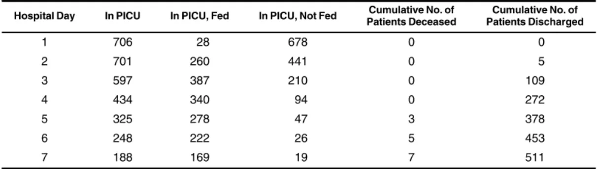
A total of 706 children were included in the study sample. Table 1shows the number of patients who were still in the PICU at each time point and, among those, the number of pa-tients receiving less than 20% of their daily caloric target (not Am J Epidemiol. 2017;186(12):1370–1379
fed) and those receiving at least 20% (fed). Table2shows the numbers of patients observed to have followed each static regime of interest, up to a given day. Figure1contrasts the static regimes“never feed”and“feed from day 3,”showing the naive estimates, not adjusted for any observed confound-ers (Figure 1A), and the IPTW (Figure1B), g-computation (Figure1C), and TMLE estimates (Figure1D). See Web Table 1 for an illustrative calculation of the naive estimates for patients who followed the regime“feed from day 3.”
The naive estimates indicate a significantly higher probabil-ity of being discharged by each day for the“never feed”regime as compared with the“feed from day 3”regime. For example, the probability of discharge by the end of day 5 is 0.88 (95% confidence interval (CI): 0.87, 0.90) for“never feed,”in con-trast to the significantly lower estimate of 0.64 (95% CI: 0.62, 0.66) for“feed from day 3.”Adjustment for baseline and time-varying confounders shifts the estimated probability of discharge in each time period downwards and reduces the difference between the two regimes. Using TMLE, we estimated a 0.66 probability of discharge by the end of day 5 for children who were never fed (95% CI: 0.59, 0.72) and a 0.53 probability for those who were fed from day 3 (95% CI: 0.48, 0.59). The TMLE, IPTW, and g-computation estimators produced similar point estimates, while TMLE generated narrower 95% confi -dence intervals than the IPTW estimator. For example, the prob-ability of discharge by the end of day 5 for the“feed from day
3”regime was estimated to be 0.54 (95% CI: 0.47, 0.60) using IPTW and 0.59 using g-computation. The smallest estimated cumulative probability of following a given regime, across all of the regimes considered, was more than 0.05, so no weight trun-cation was used.
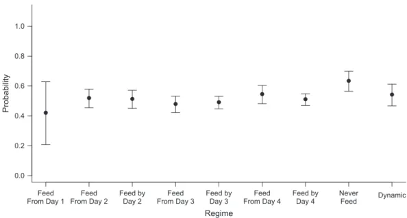
Focusing on the cumulative probability of discharge by day 4, Figure2contrasts the intervention-specific mean estimates across all regimes distinguishable by this time point, estimated by TMLE. The estimated probability for the static regime“feed from day 1”is 0.42, with the widest 95% confidence interval among all regimes (95% CI: 0.21, 0.62), which can be explained by the low number of patients following this regime. Regimes requiring starting feeding from the third day onward or by the third day, compared with starting on the second day, have lower expected probabilities of discharge; however, the 95% confi -dence intervals overlap. As before, the regime“never feed”has the most favorable expected outcomes (TMLE producing an estimated probability of discharge of 0.63 (95% CI: 0.57, 0.79)); however, the probability of discharge under this regime is not statistically significantly different from that under the other regimes.
DISCUSSION
We implemented a doubly robust approach, TMLE, to con-trast the counterfactual probability of being discharged alive
Table 2. Cumulative Numbers of Patients Whose Data Were Consistent With Each Static Feeding Regime (n=706), CHiP Study, 2008–2011
Hospital Day Feed From . . . Never Feed
Day 1 Day 2 Day 3 Day 4 Day 5 Day 6 Day 7
1 28 678 678 678 678 678 678 678 2 24 241 442 442 442 442 442 442 3 24 220 254 270 270 270 270 270 4 22 212 237 205 197 197 197 197 5 21 205 232 195 178 173 173 173 6 21 202 226 192 176 165 165 165 7 21 200 223 186 175 164 163 162
Abbreviation: CHiP, Control of Hyperglycemia in Paediatric Intensive Care.
Table 1. Patient Flow on Each Hospital Day, by Treatment Status and Outcome (n=706), CHiP Study, 2008–2011 Hospital Day In PICU In PICU, Fed In PICU, Not Fed Cumulative No. of
Patients Deceased Cumulative No. of Patients Discharged 1 706 28 678 0 0 2 701 260 441 0 5 3 597 387 210 0 109 4 434 340 94 0 272 5 325 278 47 3 378 6 248 222 26 5 453 7 188 169 19 7 511
from the PICU under a set of static and dynamic longitudinal feeding regimes in a population of critically ill children. While the unadjusted estimates showed a significant difference in discharge probabilities between the treatment regimes“start feeding from the third day”and“never feed,”after adjustment most of this difference disappeared. TMLE estimators pro-duced narrower confidence intervals than IPTW, as predicted by theory (17), while influence-curve-based confidence inter-vals for g-computation estimators were not readily available. We found no strong evidence that high levels of caloric intake may lead to adverse health outcomes in critically ill children. While in this paper the 3 statistical approaches led to similar conclusions, depending on the setting, TMLE may give sub-stantially different results from estimation methods that are not doubly robust or do not exploit data-adaptive model selec-tion (see, for example, Decker et al. (27) for an application and Schnitzer et al. (28) for simulation evidence).
An observational analysis of data from a clinical trial enabled us to investigate the impact of alternative longitudinal feeding practices on clinical outcomes. We contributed to the literature on application of longitudinal causal methods in the PICU set-ting, where, due to the fast-changing prognosis of patients and subsequently updated treatment decisions, time-dependent
confounding is an important concern (58). Using clinical judge-ment on meaningful longitudinal treatjudge-ment regimes, we selected a range of static and dynamic interventions which were sup-ported by the data, and asked new causal questions. While data collected in a clinical trial can provide advantages, such as regu-lar intervals of follow-up, measurement of a rich set of observed and time-varying confounders, and little missing data, the approach taken generalizes to settings of observational data.
This paper further provides a demonstration of the application of TMLE for longitudinal static and dynamic regimes and high-lights how it builds on alternative approaches such as IPTW and g-computation, under the challenging circumstances of a real-world comparative effectiveness study: a large number of covar-iates to adjust for and a medium-sized sample. Application of the methods to address an unanswered clinical question of high relevance in intensive care raised several methodological issues. Beyond static and dynamic treatment regimes, we also con-sidered interventions with a delayed start (e.g., “feed by day 3”) motivated by clinical practice. The availability of daily measurements of time-varying confounders resulted in high dimensionality of observed covariates to adjust for. Informed by clinical judgement, we assumed that the deci-sion as to whether to feed on a given day is influenced only 0.0 0.2 0.4 0.6 0.8 1.0 Time, days Probability 1 2 3 4 5 6 7 ● Never Feed Feed From Day 3
0.0 0.2 0.4 0.6 0.8 1.0 Time, days Probability 1 2 3 4 5 6 7 0.0 0.2 0.4 0.6 0.8 1.0 Time, days Probability 1 2 3 4 5 6 7 0.0 0.2 0.4 0.6 0.8 1.0 Time, days Probability 1 2 3 4 5 6 7 A) B) C) D)
Figure 1. Estimated cumulative probabilities of discharge from the pediatric intensive care unit by the end of days 1–7 for the feeding regime“never feed”versus“feed from day 3,”based on data from the Control of Hyperglycemia in Paediatric Intensive Care (CHiP) Study (32), 2008–2011. A) Unad-justed estimates and 95% confidence intervals (bars); B) inverse probabaility of treatment weighting estimates and 95% confidence intervals (bars); C) G-computation estimates; D) targeted maximum likelihood estimates and 95% confidence intervals (bars). Thexaxis shows time in days, while the
yaxis displays the estimated counterfactual probability of discharge from the pediatric intensive care unit, by the end of a given day, for a given regime. The 95% confidence intervals for the g-computation estimates are not reported.
Am J Epidemiol. 2017;186(12):1370–1379
by observed characteristics measured on the given day and on the previous day. To deal with the challenge of model spec-ification, we used the data-adaptive algorithm Super Learner.
Each of the methods applied here relies on the assumption that in each period, all time-constant and time-varying confound-ers that can influence treatment assignment and the outcome are observed. While the CHiP trial recorded data on a rich set of covariates, a patient’s prognosis changes quickly over time, and the observed time-varying characteristics (mechanical ventila-tion, renal replacement, inotrope score) may not capture all con-founders. In particular, if a clinician expects a patient to be discharged from the PICU soon, he or she may temporarily decrease or not initiate enteral feeding, to prevent delay in discharge. Further research using methods to analyze the sensi-tivity of the parameter estimates to the presence of unobserved confounders is therefore warranted (59).
In summary, this paper illustrates that existing data sources, such as well-conducted randomized controlled trials, can be exploited to address important questions of clinical decision-making beyond those originally posed. A wider use of appro-priate causal methods could add to the understanding of the advantage of alternative sequencing of time-varying treat-ments and could provide estimates of the effectiveness and cost-effectiveness of realistic treatment strategies.
ACKNOWLEDGMENTS
Author affiliations: Centre for Health Economics, University of York, York, United Kingdom (Noemi Kreif); Division of Biostatistics, School of Public Health,
University of California, Berkeley, Berkeley, California (Linh Tran, Maya Petersen); Centre for Statistical
Methodology, London School of Hygiene and Tropical Medicine, London, United Kingdom (Richard Grieve, Bianca De Stavola); Department of Health Services Research and Policy, London School of Hygiene and Tropical Medicine, London, United Kingdom (Richard Grieve); Department of Medical Statistics, London School of Hygiene and Tropical Medicine, London, United Kingdom (Bianca De Stavola); Department of
Anesthesiology, Perioperative and Pain Medicine, Division of Critical Care, Boston Children’s Hospital, Boston, Massachusetts (Robert C. Tasker); and Department of Neurology, Boston Children’s Hospital, Boston, Massachusetts (Robert C. Tasker).
N.K. was supported by the Medical Research Council (Early Career Fellowship in the Economics of Health MR/ L012332/1).
We thank Dr. Mark van der Laan and Josh Schwab for expert advice and Dr. Elizabeth Allen for data access.
Conflict of interest: none declared.
REFERENCES
1. Hernán MA. Counterpoint: epidemiology to guide decision-making: moving away from practice-free research.Am J Epidemiol. 2015;182(10):834–839.
2. Robins J. A new approach to causal inference in mortality studies with a sustained exposure period—application to control of the healthy worker survivor effect.Math Model. 1986;7(9–12):1393–1512.
3. Robins JM. Information recovery and bias adjustment in proportional hazards regression analysis of randomized trials using surrogate markers. In:1993 Proceedings of the Biopharmaceutical Section: Papers Presented at the Annual 0.0 0.2 0.4 0.6 0.8 1.0 Regime Probability Feed From Day 1 Feed From Day 2 Feed by Day 2 Feed From Day 3 Feed by Day 3 Feed From Day 4 Feed by Day 4 Never Feed Dynamic
Figure 2. Estimated cumulative probabilities of discharge from the pediatric intensive care unit by the end of day 4, based on data from the Control of Hyperglycemia in Paediatric Intensive Care (CHiP) Study (32), 2008–2011. Thexaxis displays the regimes compared, while theyaxis displays the targeted maximum likelihood estimates and corresponding 95% confidence intervals (bars) for the counterfactual probabilities of discharge by the end of day 4 for a given feeding regime.“Dynamic”=feed when off mechanical ventilation.
Meeting of the American Statistical Association, San Francisco, California, August 8–12, 1993, Under the Sponsorship of the Biopharmaceutical Section. (Proceedings of the Biopharmaceutical Section, American Statistical Association, vol. 24). Alexandria, VA: American Statistical Association; 1993:24–33.
4. Murphy SA, van der Laan M, Robins JM. Marginal mean models for dynamic regimes.J Am Stat Assoc. 2001;96(456): 1410–1423.
5. Murphy SA. Optimal dynamic treatment regimes.J R Stat Soc Series B Stat Methodol. 2003;65(2):331–355.
6. Chakraborty B, Murphy SA. Dynamic treatment regimes.
Annu Rev Stat Appl. 2014;1:447–464.
7. Murphy SA. An experimental design for the development of adaptive treatment strategies.Stat Med. 2005;24(10): 1455–1481.
8. Bembom O, van der Laan MJ. Analyzing sequentially randomized trials based on causal effect models for realistic individualized treatment rules.Stat Med. 2008;27(19): 3689–3716.
9. Parmar MK, Carpenter J, Sydes MR. More multiarm randomised trials of superiority are needed.Lancet. 2014; 384(9940):283–284.
10. Hernán MA, Robins JM. Using big data to emulate a target trial when a randomized trial is not available.Am J Epidemiol. 2016;183(8):758–764.
11. Robins JM, Hernán MA, Brumback B. Marginal structural models and causal inference in epidemiology.Epidemiology. 2000;11(5):550–560.
12. Daniel RM, Cousens S, De Stavola BL, et al. Methods for dealing with time-dependent confounding.Stat Med. 2013; 32(9):1584–1618.
13. Cain LE, Robins JM, Lanoy E, et al. When to start treatment? A systematic approach to the comparison of dynamic regimes using observational data.Int J Biostat. 2010;6(2):Article 18. 14. Horvitz DG, Thompson DJ. A generalization of sampling
without replacement from afinite universe.J Am Stat Assoc. 1952;47(260):663–685.
15. Petersen ML, Porter KE, Gruber S, et al. Diagnosing and responding to violations in the positivity assumption.Stat Methods Med Res. 2012;21(1):31–54.
16. Robins JM, Blevins D, Ritter G, et al. G-estimation of the effect of prophylaxis therapy forPneumocystis carinii
pneumonia on the survival of AIDS patients.Epidemiology. 1992;3(4):319–336.
17. van der Laan MJ, Rubin D. Targeted maximum likelihood learning.Int J Biostat. 2006;2(1):1–38.
18. Gruber S, van der Laan MJ. A targeted maximum likelihood estimator of a causal effect on a bounded continuous outcome.
Int J Biostat. 2010;6(1):Article 26.
19. Van der Laan MJ, Rose S.Targeted Learning: Causal Inference for Observational and Experimental Data. New York, NY: Springer-Verlag; 2011.
20. Zheng W, van der Laan MJ. Targeted maximum likelihood estimation of natural direct effects.Int J Biostat. 2012;8(1):1–40. 21. van der Laan MJ, Gruber S. Targeted minimum loss based
estimation of causal effects of multiple time point interventions.Int J Biostat. 2012;8(1):1–39.
22. Petersen M, Schwab J, Gruber S, et al. Targeted maximum likelihood estimation for dynamic and static longitudinal marginal structural working models.J Causal Inference. 2014; 2(2):147–185.
23. van der Laan MJ, Dudoit S, Keles S. Asymptotic optimality of likelihood-based cross-validation.Stat Appl Genet Mol Biol. 2004;3(1):Article 4.
24. van der Laan MJ, Polley EC, Hubbard AE. Super learner.Stat Appl Genet Mol Biol. 2007;6(1):Article 25.
25. Schuler MS, Rose S. Targeted maximum likelihood estimation for causal inference in observational studies.Am J Epidemiol. 2017;185(1):65–73.
26. Bang H, Robins JM. Doubly robust estimation in missing data and causal inference models.Biometrics. 2005;61(4):962–973. 27. Decker AL, Hubbard A, Crespi CM, et al. Semiparametric
estimation of the impacts of longitudinal interventions on adolescent obesity using targeted maximum-likelihood: accessible estimation with the ltmle package.J Causal Inference. 2014;2(1):95–108.
28. Schnitzer ME, van der Laan MJ, Moodie EE, et al. Effect of breastfeeding on gastrointestinal infection in infants: a targeted maximum likelihood approach for clustered longitudinal data.
Ann Appl Stat. 2014;8(2):703–725.
29. Tran L, Yiannoutsos CT, Musick BS, et al. Evaluating the impact of a HIV low-risk express care task-shifting program: a case study of the targeted learning roadmap.Epidemiol Methods. 2016;5(1):69–91.
30. Brown DM, Petersen M, Costello S, et al. Occupational exposure to PM2. 5and incidence of ischemic heart disease:
longitudinal targeted minimum loss-based estimation.
Epidemiology. 2015;26(6):806–814.
31. Neugebauer R, Schmittdiel JA, van der Laan MJ. Targeted learning in real-world comparative effectiveness research with time-varying interventions.Stat Med. 2014;33(14):2480–2520. 32. Macrae D, Grieve R, Allen E, et al. A randomized trial of
hyperglycemic control in pediatric intensive care.N Engl J Med. 2014;370(2):107–118.
33. Petersen ML, van der Laan MJ. Causal models and learning from data: integrating causal modeling and statistical estimation.Epidemiology. 2014;25(3):418–426. 34. McClave SA, Martindale RG, Rice TW, et al. Feeding the
critically ill patient.Crit Care Med. 2014;42(12):2600–2610. 35. Mehta NM, Compher C; A.S.P.E.N. Board of Directors.
A.S.P.E.N. Clinical Guidelines: nutrition support of the critically ill child.JPEN J Parenter Enteral Nutr. 2009;33(3):260–276. 36. Fivez T, Kerklaan D, Mesotten D, et al. Early versus late
parenteral nutrition in critically ill children.N Engl J Med. 2016;374(12):1111–1122.
37. Gerrior S, Juan W, Peter B. An easy approach to calculating estimated energy requirements.Prev Chronic Dis. 2006;3(4): A129.
38. Al-Radi OO, Harrell FE Jr, Caldarone CA, et al. Case complexity scores in congenital heart surgery: a comparative study of the Aristotle Basic Complexity score and the Risk Adjustment in Congenital Heart Surgery (RACHS-1) system.
J Thorac Cardiovasc Surg. 2007;133(4):865–875.
39. Wernovsky G, Wypij D, Jonas RA, et al. Postoperative course and hemodynamic profile after the arterial switch operation in neonates and infants. A comparison of low-flow
cardiopulmonary bypass and circulatory arrest.Circulation. 1995;92(8):2226–2235.
40. Hernán MA, Lanoy E, Costagliola D, et al. Comparison of dynamic treatment regimes via inverse probability weighting.
Basic Clin Pharmacol Toxicol. 2006;98(3):237–242. 41. Young JG, Cain LE, Robins JM, et al. Comparative
effectiveness of dynamic treatment regimes: an application of the parametric g-formula.Stat Biosci. 2011;3(1): 119–143.
42. Snowden JM, Rose S, Mortimer KM. Implementation of G-computation on a simulated data set: demonstration of a causal inference technique.Am J Epidemiol. 2011;173(7): 731–738.
Am J Epidemiol. 2017;186(12):1370–1379
43. Petersen ML. Commentary: applying a causal road map in settings with time-dependent confounding.Epidemiology. 2014;25(6):898–901.
44. Robins JM. Analytic methods for estimating HIV-treatment and cofactor effects. In: Ostrow DG, Kessler RC, eds.
Methodological Issues in AIDS Behavioral Research. New York, NY: Plenum Press; 2002:213–288.
45. Robins JM. Commentary on“using inverse weighting and predictive inference to estimate the effects of time-varying treatments on the discrete-time hazard.”Stat Med. 2002; 21(12):1663–1680.
46. Robins J, Sued M, Lei-Gomez Q, et al. Comment: performance of double-robust estimators when“inverse probability” weights are highly variable.Stat Sci. 2007;22(4):544–559. 47. van der Laan MJ, Dudoit S.Unified Cross-Validation
Methodology for Selection Among Estimators and a General Cross-Validated Adaptive Epsilon-Net Estimator: Finite Sample Oracle Inequalities and Examples. (Working Paper 130). Berkeley, CA: Berkeley Electronic Press; 2003.http://biostats. bepress.com/ucbbiostat/paper130. Accessed January 16, 2016. 48. Hastie T.gam: Generalized Additive Models. (R package,
version 1.09). Vienna, Austria: R Foundation for Statistical Computing; 2013.http://CRAN.R-project.org/package=gam. Accessed April 30, 2015.
49. Gelman A, Su YS.arm: Data Analysis Using Regression and Multilevel/Hierarchical Models. (R package, version 1.6-09). Vienna, Austria: R Foundation for Statistical Computing; 2013.http://CRAN.R-project.org/package=arm. Accessed April 30, 2015.
50. Simon N, Friedman J, Hastie T, et al. Regularization paths for Cox’s proportional hazards model via coordinate descent.
J Stat Softw. 2011;39(5):1–13.
51. Ridgeway G, et al.gbm: Generalized Boosted Regression Models. (R package, version 2.1.3). Vienna, Austria: R Foundation for Statistical Computing; 2006.https://cran. r-project.org/web/packages/gbm/index.html. Accessed April 30, 2015.
52. Venables WN, Ripley BD.Modern Applied Statistics With S. 4th ed. New York, NY: Springer Publishing Company; 2002. 53. Tsiatis A.Semiparametric Theory and Missing Data. New
York, NY: Springer Publishing Company; 2006. 54. Hampel FR, Ronchetti EM, Rousseeuw PJ, et al.Robust
Statistics: The Approach Based on Influence Functions. New York, NY: John Wiley & Sons, Inc.; 2011.
55. Schwab J, Lendle S, Petersen M, et al.ltmle: Longitudinal Targeted Maximum Likelihood Estimation. (R package, version 0.9-9). Vienna, Austria: R Foundation for Statistical Computing; 2015.https://cran.r-project.org/web/packages/ ltmle/index.html.Accessed December 29, 2016.
56. R Core Team.The R Project for Statistical Computing. Vienna, Austria: R Foundation for Statistical Computing; 2016.https:// www.R-project.org/. Accessed December 29, 2016.
57. Polley E, van der Laan M.SuperLearner: Super Learner Prediction. (R package, version 2.0-10). Vienna, Austria: R Foundation for Statistical Computing; 2013. http://CRAN.R-project.org/package=SuperLearner. Accessed December 29, 2016.
58. Vansteelandt S, Mertens K, Suetens C, et al. Marginal structural models for partial exposure regimes.Biostatistics. 2009;10(1):46–59.
59. Brumback BA, Hernán MA, Haneuse SJ, et al. Sensitivity analyses for unmeasured confounding assuming a marginal structural model for repeated measures.Stat Med. 2004;23(5): 749–767.