GRIPS Discussion Paper 15-17
Efficient Bayesian Inference in Generalized Inverse Gamma
Processes for Stochastic Volatility
Roberto Leon-Gonzalez
October 2015
National Graduate Institute for Policy Studies 7-22-1 Roppongi, Minato-ku,
E¢ cient Bayesian Inference in Generalized Inverse Gamma
Processes for Stochastic Volatility
Roberto Leon-Gonzalez
National Graduate Institute for Policy Studies (GRIPS)
This version: July 2015
(First version: September 2014)
Abstract
This paper develops a novel and e¢ cient algorithm for Bayesian inference in inverse Gamma Stochastic Volatility models. It is shown that by conditioning on auxiliary variables, it is possible to sample all the volatilities jointly directly from their posterior conditional density, using simple and easy to draw from distributions. Furthermore, this paper develops a generalized inverse Gamma process with more ‡exible tails in the distribution of volatilities, which still allows for simple and e¢ cient calculations. Using several macroeconomic and …nancial datasets, it is shown that the inverse Gamma and Generalized inverse Gamma processes can greatly outperform the commonly used log normal volatility processes with student-t errors.
JEL: C11, C15
Keywords: Markov Chain Monte Carlo, Gibbs Sampling, Flexible Parametric Models, Particle Filters.
I thank the Japan Society for the Promotion of Science for …nancial support under the Young-Scientist (B) Grant (#23730214 and #26780135). I thank participants of the Statistics & Econometrics Workshop of Hitotsubashi University, DSSR workshop of Tohoku University, ISBA 2012 World Meeting in Kyoto, the CFE 2012 in Oviedo, the RCEA 2014 in Rimini, EEA 2014 in Gran Canaria and IMS-APRM 2014 in Taiwan. The author is also a fellow of the Rimini Centre for Economic Analysis (RCEA).
1
Introduction
There is overwhelming empirical evidence in favor of Stochastic Volatility models with both macroeconomic (e.g. Sims and Zha 2006) and …nancial data (e.g. Kim et al. (1998)). The …rst algorithms for posterior simulation where developed for the case in which the volatility 2
t follows an autoregressive log-normal process. The …rst algorithms used a single-move update for the volatilities (e.g. Jacquier, Polson and Rossi (1994)), which implies that 2
t is generated conditionally on the volatility values in other periods ( 2
1; :::; 2t 1; 2t+1; :::; 2T). To improve the convergence speed, it was later proposed to sample several of the volatility values at a time using blocking strategies (e.g. Shephard and Pitt (1997), Watanabe and Omori (2004), Asai (2005)). In an in‡uential paper, Kim et al. (1998) showed that by accurately approximating the likelihood with a mixture of normals, it is possible to draw jointly all the latent log-volatilities given some auxiliary variables. Furthermore, the log-volatilities can be integrated out when drawing the unknown parameters.
A more recent literature provides methods for Bayesian inference in models where 2
t follows some type of gamma or inverse gamma process. In a multivariate stochastic volatility context, Philipov and Glickman (2006) proposed a single-move algorithm whereas Fox and West (2011) proposed to sample all the volatility matrices jointly in a Metropolis-step which conditions on auxiliary variables. Creal (2012), in the univari-ate context, proposed maximum likelihood estimation by accurunivari-ately approximating the likelihood with a …nite state Markov-switching model. In the multivariate context Casarin and Sartore (2007) proposed se-quential monte carlo and particle …lters for estimation of the states and parameters and Triantafyllopoulos (2010) proposed a simpli…ed Wishart stochastic volatility model which allows for fast and simple computa-tions. Abraham et al. (2006) proposed method of moments estimators for gamma type univariate stochastic volatility models and Gourieroux et al. (2009) develop maximum likelihood inference for a Wishart autore-gressive process for observed volatility. There is also a recent literature that deals with Ornstein-Ulhlenbeck processes with marginal gamma laws (e.g. Barndor¤-Nielsen and Shephard (2001), Roberts et al. (2004), Gri¢ n and Steel (2006a), Frühwirth-Schnatter and Sögner (2009)).
A related strand of literature proposes ‡exible models for stochastic volatility. Although there are many papers that provide alternative methods to model ‡exibly the distribution of the observed dependent variable (e.g. Steel (1998), Durham (2007), Jensen and Maheu (2010), Delatola and Gri¢ n (2011), Gri¢ n and Steel (2011)), there are few that model ‡exibly the distribution of the unobserved volatility. As argued by Janssen and Drees (2013), the latter approach is more appropriate in datasets that exhibit persistence of volatility outliers. In this line Gri¢ n and Steel (2006b) and Jensen and Maheu (2014) provide semiparametric methods of inference based on in…nite mixtures for the volatility distribution. However, there is a lack of models
that specify the volatility process in a ‡exible yet parametric manner. Flexible parametric models could potentially perform better than semiparametric ones in some datasets, while taking advantage of simpler and more e¢ cient computational methods.
The purpose of this paper is to develop e¢ cient posterior simulators for ‡exible inverse gamma stochastic volatility models. We show that by conditioning on some auxiliary variables, it is possible to draw all the volatilities jointly using simple distributions such as the Poisson and Gamma. Furthermore, it is possible to generate the unknown parameters after integrating out all the volatilities. Because of these features, our algorithm mimicks the e¢ cient algorithm that Kim et al (1998) developed for the lognormal model, without requiring the use of an approximation to the likelihood. Moreover, this paper proposes a generalized inverse gamma time-series model that speci…es a more ‡exible distribution for the volatility, allows for more abrupt jumps in volatility, and can be estimated using simple and e¢ cient methods. In an empirical exercise we show that the generalized inverse gamma process is especially suitable to model series with greater volatility jumps and persistence in outliers. Furthermore, we use real and simulated data to illustrate the e¢ ciency of the new algorithm and show that it is much more e¢ cient than the recently proposed Particle Markov Chain Monte Carlo methods (Andrieu et al. 2010) which sample the volatilities and parameters in a joint move using a particle …lter.
This paper di¤ers from previous work on gamma type stochastic volatility models in two main aspects. Firstly, we …nd a method to sample all the volatilities jointly from the posterior using well-known distributions such as the Poisson and Gamma, whereas previous work mostly used single-move or blocking strategies in a Metropolis-step to sample the volatilities. As mentioned before, sampling the volatilities jointly from the posterior is an important characteristic of e¢ cient algorithms. Secondly, we develop and study the properties of a ‡exible inverse gamma time series model that can be estimated with simple and e¢ cient computations. Thus this paper provides a new class of ‡exible stochastic volatility models that can be estimated with simple and e¢ cient MCMC methods.
Section 2 describes the inverse gamma and generalized inverse gamma processes and Section 3 develops the posterior simulators. Section 4 presents evidence on the computational e¢ ciency of the algorithms and Section 5 compares the empirical performance of di¤erent models using several macroeconomic and …nancial datasets. Section 6 concludes.
2
Models
2.1
The Autoregressive Gamma Process (ARG)
We consider the following model of stochastic volatility:
yt = xt + tet
et N(0;1)
Although for simplicity in the exposition we are assuming normality foret, in the empirical applications we will consider also models whereetfollows a student-t. The student-t can be easily incorporated into this framework by writing it as a scale mixture of normals, as in Chib et al (2002). The stochastic process for the volatility 2
t can be described by de…ning kt= t2 and assuming that kt= z0tzt, where zt is a n 1 vector distributed as a Gaussian AR(1) process:
zt= zt 1+"t "t N(0; 2In) (1)
Equation (1) implies that the conditional distribution of(kt= 2)jkt 1is a noncentral chi squared, which is
also well de…ned for non-integer values ofn, and therefore we will treatnas a continuous unknown parameter. The joint distribution of (k1; :::; kT) is the multivariate gamma distribution analyzed by Krishnaiah and Rao (1961). It was proposed for observed volatility (or intertrade durations) by Gourieroux and Jasiak (2006) and for unobserved volatility by Creal (2012). In our case we are using it for the inverse of the unobserved volatility, as this makes Bayesian computations simpler. This is in line with the Bayesian analysis of Fox and West (2011), who specify a Wishart distribution for the inverse volatility matrix. However, although the stationary distribution of 2t is the same as in Fox and West (2011), the transitional density 2tj 2t 1 is
di¤erent.
The properties of (k1; :::; kT) are well known (e.g. Krishnaiah and Rao (1961), Gourieroux and Jasiak (2006)) and the most important ones can be summarized as:
E(kt) = n 2 1 2,E(kt2) = 2 1 2 2 n(n+ 2) corr(kt; kt h) = 2h E(ktjkt 1) = 2kt 1+ (1 2)E(kt) The conditional distribution kt
The stationary distribution of kt is a G(n=2; 2
2
1 2), where G(:) represents the gamma distribution
(Bauwens et al. (1999, p. 290)).
A necessary and su…cient condition for stationarity isj j<1
In addition, the properties of ( 2
1; :::; 2T) can be derived from the properties of (k1; :::; kT) as explained at the end of the proof of Proposition 1, so that we obtain:
E( 2 t) = 1 2 2(n 2) forn >2,var( 2t) = E( 2t) 2 2 n 4 forn >4 corr( 2
t; 2t h) = (n=2 2)[2F1(1;1;n=2; 2h) 1], for n >4, where2F1(:) is a hypergeometric series
(e.g. Slater (1966, p. 1)). E( 2 tj 2t 1) = 2(n1 2)[1F1(1;n=2; 2 2 2 2 t 1], forn >2.
The stationary distribution of 2
t is a IG2(1
2
2 ; n), where IG2(:) represents the inverted gamma
distribution (Bauwens et al. (1999, p. 292)).
From the properties of the hypergeometric series it can be shown that the correlation corr( 2t; 2t h)is
0 when = 0 and it is equal to1 when = 1(e.g. Slater (1966, p.2)). In the following it will be assumed that k1 is drawn from the stationary distribution, that isk1 G(n=2;2 2=(1 2)). Note …nally that the
autocorrelations are de…ned by 2, so that they cannot be negative. In fact enters the likelihood always in
the form of 2, so that the sign of is not identi…ed. For this reason in our empirical section we will specify
the prior not on but directly on 2.
2.2
Flexible Tail Autoregressive Gamma Process (FTARG)
The parameters (n; 2; 2) control the unconditional mean, variance and the …rst order correlation of k
t. However, the degrees of freedomn also control the shape of the tails of the distribution ofk and therefore it also controls the tails of the distribution ofy. Hence it might be desirable to consider models where the shape of the tails is not determined by the …rst two unconditional moments ofkt. There is previous literature that develops more ‡exible gamma-type distributions, such as the generalized gamma distribution of Stacy (1962) or the compound gamma of Dubey (1970) (see also Johnson et al. (1994, section 17.8) for a review). However, here we propose a di¤erent type of distribution that lends itself better to the context of time-series and the use of MCMC methods for computation. For this purpose we de…ne the Flexible Tail Autoregressive Gamma Process (FTARG). Recall thatkt=zt0zt. Instead ofzt= zt 1+"twe now assume:
zt= q
e
where(Te2; :::;TeT)are independent draws from a Beta distributionB( ; ). Given that we are more concerned with modelling the left tail ofkt(which corresponds to the right tail of 2t) and given that the stationarity of the process requiresE(Tet)<1= 2, it seems appropriate to specify a distribution with bounded support forTet. If we writeet=
q e
Ttande
2
t =Tet 2 it is clear that the FTARG process arises from (1) by writing etinstead of ande2t instead of 2, and therefore the FTARG is equivalent to the ARG with time-varying parameters. Furthermore, the FTARG can be also compared to the ARG process by de…ninge=
q
E(Tet) , e2=E(Tet) 2 ande"t N(0;e
2
), such that (2) can be equivalently written as:
zt= s e Tt E(Tet) (ezt 1+e"t) so thatkt=zt0ztbecomes: kt= e Tt E(Tet) (ezt 1+e"t)0(ezt 1+e"t) (3)
From this expression it is clear that whenTet > E(Tet) (Tet < E(Tet)), the value of kt is higher (lower) than in the ARG model, which adds ‡exibility to the model. Furthermore, when the variance ofTet approaches
0, the ratioTet=E(Tet)behaves as a constant of value 1, and therefore the FTARG becomes equivalent to the ARG. However this implies that when the variance ofTetis close to0, the mean ofTetis poorly identi…ed. To avoid this local non-identi…cation problem, we …x E(Tet) = 1=2. For this purpose, we reparameterize( ; ) as A=E(Tet) = =( + ) and V = ( + ), and …xA= 1=2. Therefore with this normalization we have that = =V =2. The parameterV controls the variance of Tet and will be estimated.
The properties of the FTARG can be derived using basic properties of the gamma and beta distributions and are summarized in the following proposition whose proof is in the appendix.
Proposition 1 De…nee2=E(Tet) 2 ande
2
=E(Tet) 2. The main properties of(k1; :::; kT)and( 21; :::; 2T)
implied by (2) are: E(ktjkt 1) = e2kt 1+ (1 e2)E(kt) ife2<1 (4) corr(kt; kt h) = e2h if e2<1 (5) corr( 2t; 2t h) = (n=2 2)[2F1(1;1;n=2; 2h) 1]; for n >4 (6) E(ktjkt 1;Tet) = e Tt E(Tet) (e2kt 1+ (1 e2)E(kt)) (7) E(kt) = ne2 1 e2 ife 2 <1 (8) E(k2t) = 2 2n(n+ 2)E(v2c;t) if 4E(Tet2)<1 (9)
where vc;t=Tet(1 + 2Tet 1+ 4Tet 1Tet 2+ 6Tet 1Tet 2Tet 3+:::)and: E(v2c;t) = E(Te 2 t)(1 +e2) (1 e2)(1 4E(Te2 t)) if 4E(Tet2)<1
Higher moments ofktare given by:
E(kts) =E(vsc;t) 2 s
sY1
i=0
(n+ 2i)if 2sE(Tets)<1
whereE(vs
c;t)can be calculated recursively as:
E(vc;ts ) = E(Te s t) 1 2sE(Tes t) s 1 X i=0 s i 2iE(vi c;t) if 2sE(Tets)<1 (10)
and where the properties of the Beta distribution imply that:
E(Tets) =
sY1
i=0
+i
+ +i
The stationary distribution ofkt is that of the product of "0t"t (i.e. a gamma distribution) and vc;t, where
"0
t"andvc;t are independent of each other. ThesthmomentE( 2t s
) =E(kts)is …nite if and only if > s
andn >2s.
SinceE(Tet)is normalized to be1=2, the condition for the …rst order moment of the stationary distribution of kt to be …nite is 2 <2 However, the existence of higher moments of kt requires a tighter restriction on 2. In the empirical analysis of Section 5 we only impose the restriction 2<2, implying that the …rst
order correlation coe¢ cient e2 is allowed to vary on the whole range of the interval (0;1). Note also that the restriction 2 < 2 is su¢ cient for 2
t (i.e. the inverse of kt) to have …nite moments up to the order
min( ; n=2).
Equation (4) indicates that the conditional expectation of kt given kt 1 is a weighted average of kt 1
and the unconditional meanE(kt), as in a standard AR(1) model. Furthermore, equation (5) indicates that the autocorrelation structures of the ARG and the FTARG are the same.
The expression for E(ktjkt 1;Tet) in equation (7) indicates that when Tet > E(Tet) (Tet < E(Tet)) the expected value ofktjkt 1is above (below) what would be expected in the ARG model, making the tails more
‡exible. In particular, very small values ofTetwill imply low values forktand consequently very large values for the volatility 2
t. As we will see in the empirical section, this feature makes the FTARG model specially useful for data with periods of greater instability.
conditional distribution ofktjkt 1can be written as a GammaG(n=2 +ht;2 2Tet), wherehtfollows a Poisson distribution P( t) with t = 2kt 1=2 2 and Tet follows a beta distribution (as described in Section 3.1). Therefore we are generalizing the conditional distribution of ktjkt 1 by using a scale mixture of gammas,
in which the mixing distribution is a beta distribution. Similarly, the stationary distribution of kt is a scale mixture of Gammas, where the mixing distribution is that ofvc;t. Note that restricting the support of Tet to (0;1) does not restrict the support of vc;t, which is unbounded. This approach to generalize the distribution is somehow analogous to the compound gamma distribution of Dubey (1970), which is also derived as a scale mixture of gammas, but with a gamma as the mixing distribution. Our framework could be further generalized by assuming thatTetfollows a discrete mixture of Beta distributions, as a mixture of beta distributions can accurately approximate any distribution on the(0;1)interval (e.g. Petrone, 1999).
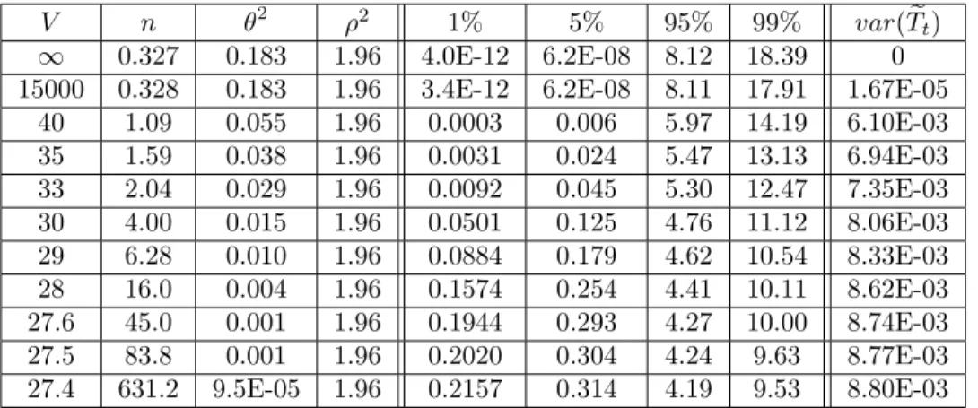
Tables 1 and 2 show howV a¤ects the percentiles of the stationary distribution ofktwhile keepingE(kt),
E(k2
t)and cov(kt; kt 1) constant. Even if the parameter for the degrees of freedom n increases from1 to
100, by decreasing V and in a suitable manner, the moments can be kept constant while the tail of the distribution varies considerably. In particular Table 1 shows that the 1% percentile varies from 0.003 to 0.45 asV varies from1to40. In Table 2 the 1% percentile varies from 3.5E-12 to 0.2157 asV varies from1to
27:4. Thus, whenV is large andnis small, the tail ofkttowards0is fatter, whereas decreasing the value of
V allowsnto be larger and in this way reduce the probability of values near0. This implies that the right tail of the volatility 2
t is fatter when V is large and n is small. To see the impact on the distribution of the volatility 2
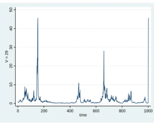
t, Figures 1 - 3 plot one random realization of( 21; :::; 21000)for 3 of the processes in Table 2
(those corresponding toV = 33,V = 29andV = 27:5). Even though the 3 processes imply the same values forE(kt), E(kt2)and cov(kt; kt 1), we can see that 2t takes occasionally very large values (larger than 800 in Figure 1) whenV = 33, but whenV = 27:5 the values for 2t in Figure 3 are all below 11. Note that the …rst moments for 2t, that isE( 2t),E(( 2t)2)andcov( 2t; 2t 1), need not be the same though Figures 1 to
3. For example the second moment of 2
t is in…nity in Figure 1, becausenis smaller than 4.
For simplicity, instead of assuming that k1 is drawn from the stationary distribution, it will be
as-sumed that k1 is drawn from a distribution which has the same mean as the stationary distribution:
k1 G(n=2;2e 2
V n 2 2 1% 5% 95% 99% var(Tet) 1 1.28 0.078 1.96 0.003 0.031 8.78 14.53 0 15000 1.29 0.078 1.96 0.003 0.032 8.85 14.61 1.7E-05 7500 1.29 0.078 1.96 0.003 0.032 8.76 14.54 3.3E-05 1000 1.34 0.075 1.96 0.003 0.036 8.77 14.50 2.5E-04 500 1.40 0.072 1.96 0.004 0.041 8.65 14.58 5.0E-04 200 1.60 0.062 1.96 0.009 0.064 8.46 14.70 1.2E-03 150 1.76 0.057 1.96 0.012 0.080 8.32 14.92 1.7E-03 100 2.16 0.046 1.96 0.028 0.125 8.02 14.74 2.5E-03 50 6.31 0.016 1.96 0.203 0.396 7.12 13.85 4.9E-03 45 10.84 0.009 1.96 0.295 0.498 6.84 13.48 5.4E-03 42 22.04 0.005 1.96 0.380 0.581 6.71 13.37 5.8E-03 41 35.34 0.003 1.96 0.412 0.613 6.63 13.24 6.0E-03 40 96.20 0.001 1.96 0.451 0.645 6.54 13.24 6.1E-03
Table 1: Percentiles of kt for di¤erent values ofV. The value of E(kt), E(kt2) and cov(kt; kt 1) are kept
equal in all cases to2:5,16and0:98, respectively. The percentiles are calculated using 150000 independent draws. The table does not show values ofV smaller than40because it is not possible to maintain the same values of (E(kt),E(kt2),cov(kt; kt 1))whenV <40.
V n 2 2 1% 5% 95% 99% var(Tet)
1 0.327 0.183 1.96 4.0E-12 6.2E-08 8.12 18.39 0
15000 0.328 0.183 1.96 3.4E-12 6.2E-08 8.11 17.91 1.67E-05
40 1.09 0.055 1.96 0.0003 0.006 5.97 14.19 6.10E-03 35 1.59 0.038 1.96 0.0031 0.024 5.47 13.13 6.94E-03 33 2.04 0.029 1.96 0.0092 0.045 5.30 12.47 7.35E-03 30 4.00 0.015 1.96 0.0501 0.125 4.76 11.12 8.06E-03 29 6.28 0.010 1.96 0.0884 0.179 4.62 10.54 8.33E-03 28 16.0 0.004 1.96 0.1574 0.254 4.41 10.11 8.62E-03 27.6 45.0 0.001 1.96 0.1944 0.293 4.27 10.00 8.74E-03 27.5 83.8 0.001 1.96 0.2020 0.304 4.24 9.63 8.77E-03 27.4 631.2 9.5E-05 1.96 0.2157 0.314 4.19 9.53 8.80E-03
Table 2: Percentiles of kt for di¤erent values ofV. The value of E(kt), E(kt2) and cov(kt; kt 1) are kept
equal in all cases to1:5,16and0:98, respectively. The percentiles are calculated using 150000 independent draws. The table does not show values of V smaller than27:4 because it is not possible to maintain the same values of(E(kt),E(k2t),cov(kt; kt 1))whenV <27:4.
0 2 00 4 00 6 00 8 00 V = 33 0 200 400 600 800 1000 time
Figure 1: One random draw of( 2
1; :::; 21000)withV = 33,n= 2:04, 2= 0:029and 2= 1:96. These values
0 10 20 30 40 50 V = 29 0 200 400 600 800 1000 time
Figure 2: One random draw of( 2
1; :::; 21000)withV = 29,n= 6:28, 2= 0:0095and 2= 1:96. The values
forE(kt),E(kt2)andcov(kt; kt 1)are the same as in Figure 1.
0 2 4 6 8 10 V = 27.5 0 200 400 600 800 1000 time
Figure 3: One random draw of( 2
1; :::; 21000) withV = 27:5,n= 83:77, 2 = 0:00072and 2= 1:96. The
3
Computation by Gibbs Sampling
3.1
Autoregressive Gamma Process (ARG)
In this section we will use the notationet=
q e Tt and e 2 t =Tet 2 for t= 2; :::; T ande1 =e = q E(Tet) , e21 =e2 =E(Tet) 2 with the understanding that in the ARG model Tet = 1 and soet = ande
2
t = 2 for everyt. In this way the conditional posterior densities derived in this section will be valid for both the ARG and the FTARG models whenTeis among the conditioning variables. As noted before, the prior of kt
e2 tj
kt 1
is a noncentral chi squared. From Muirhead (1982, p. 23) it turns out that a noncentral chi squared can be written as a mixture of (central) chi-squared with degrees of freedomn+ 2ht, where ht follows a Poisson. Using this representation, the model can be written as:
yt = xt + r 1 kt et (11) et N(0;1) ktjk1:(t 1); h1:t; ; G(n=2 +ht;2e 2 t) htjk1:(t 1);h1:(t 1); ; P( t) with t=e 2 tkt 1 2e2t
whereG(:)represents the gamma distribution (Bauwens et al. (1999), p. 290),P(:)is the Poisson distribution (Koop (2003), p. 325) andk1:(t 1) is notation for (k1; :::; k(t 1)). Let = (n; 2; 2), k = (k1; :::; kT) and
h= (h2; :::; hT). The representation (11) suggests the …rst Gibbs sampling algorithm that we consider: The h-Gibbs
Generate jh; (Metropolis step)
Generatekjh; ; (draw from independent gamma).
Generatehjk; ; (draw from independent Bessel distributions). Generate jk; h; (draw from a multivariate normal).
Note that for greater e¢ ciency is drawn marginally on k. For this reason k needs to be drawn immediately after , so that the algorithm converges to the joint posterior distribution. An advantage of this algorithm is that all the precisions in the vectorkcan be drawn jointly from the conditional posterior. Similarly, as noted by Creal (2012), the vector hcan be drawn jointly from the posterior conditional using a discrete distribution known as Bessel distribution (Yuan and Kalb‡eisch (2000)). Devroye (2002) and Iliopoulos and Karlis (2003) have developed e¢ cient algorithms to draw from the Bessel distribution. The
conditional distributions needed in the h-Gibbs algorithm are summarized in the following proposition, whose proof is in the appendix.
Proposition 2 Consider the model de…ned by (11), and de…ne:
r2t = (yt xt )2 e r2t = 1 +e 2 t e2t +r 2 t ! 1 fort= 2; :::; T 1 e r2t = 1 e2t +r 2 t ! 1 fort= 1andt=T h1 = hT+1= 0
The conditional posteriors are as follows:
ktjh; ; G((n+ 1)=2 +ht+ht+1;2er2t) fort= 1; :::; T htjk; ; Bessel( n 2 2 ;et p ktkt 1 e2t ) fort= 2; :::; T and p( jY; h; ) / Z p( )p(k; hj ; )L(Yjk; )dk= (12) (2 ) T =2 T Y t=1 2er2t n+1 2 +ht+1+ht n+ 1 2 +ht+1+ht 2 6 6 6 4 T Y t=2 1 2e2t n=2 et 2e2t 2ht ht! 1 (n=2 +ht) 3 7 7 7 5(1 e 2 )n=2 2e2 n 2 n 2 1 p( )
whereL(Yjk; )is the density function of the observed dataY given the volatilitiesk andp( )is the prior.
However, the convergence of this algorithm can be slow because of the high correlation between k and
h. Indeed, once we condition upon h, the di¤erent components ofkbecome independent of each other, even if unconditionally the serial correlation ofkt is tipically very high. This suggests thathcontains too much information aboutkand so ideally we would like to draw kandhjointly. Thus we consider a second Gibbs algorithm that surpasses this problem, and that also has the advantage of drawing from distributions that are simpler than the Bessel. For this purpose we introduce two vectors of auxiliary variables, one of them continuousm= (m2; :::; mT)and another discrete d= (d2; :::; dT), such that we will be able to draw (k; h) jointly conditioning on(m; d)and viceversa. Let us introducemtby assuming thatmtconditional onhthas
a beta distribution:
mtjht B( m+ht; m); m= (n 1)=2; m= 1=2 (13)
Note that this requiresn >1. This restriction is weaker than the condition to ensure thatE( 2
t)is …nite, which requires n >2. The advantage of this parameterization is that the posterior ofhtj(k1:(t 1); h1:(t 1);
m1:t) is a …nite mixture of shifted Poissons, whereas the posterior of ktjk1:(t 1); h1:t; m1:t continues to be a Gamma. This is what makes possible the joint sampling of the two vectors k and hconditional on m. However, the calculation of the probabilities of each component of the mixture could be time consuming, especially whenT is large. For this reason it seems preferable to condition on a mixture indicator dt, such that the conditional posterior of ht becomes simply a shifted Poisson. This implies that conditional on (m; d), the two vectorskandhcan be drawn jointly from the conditional posterior using simple gamma and shifted Poisson distributions. In turn,(m; d)j(k; h)can be drawn using independent beta distributions (for
m) and the hypergeometric distribution ford.
A shifted Poisson results from adding a …xed constant to a random variable with Poisson distribution (Winkelmann (2008, p.10)). We use the notation ht SP( t; dt)to mean that (ht dt) follows a Poisson distribution (i.e. (ht dt) P( t)). The probability density function of a shifted Poisson distribution is:
fSP(hj ; d) = h d
1 (h d)!
1
exp( ) h=d;(d+ 1); ::: (14)
Note that a draw from a shifted Poisson ht SP( t; dt) can be obtained by …rst obtaining a drawx from the Poisson distributionP( t) and then calculatinght=x+dt. The vectordis formally introduced in the model by using a hypergeometric distribution (e.g. Monahan (2001, p. 305)) as a prior for each of the components ofdgivenh:
Pr (dt=sjht; dt+1) = Mdt s Ndt Mdt ndt s Ndt ndt t= 2; :::; T dT+1= 0 0 s min((1 +dt+1); ht) (15) Mdt = ht; ndt = 1 +dt+1; Ndt = (n 1)=2 +ht+dt+1
Because in our caseNdt is not an integer, the corresponding binomial coe¢ cient should be written using the gamma function instead of the factorial, based on the relationship (x+1) =x!(see proof of Proposition 3 in the appendix for more details). There are several algorithms that e¢ ciently draw from the hypergeometric
distribution, are available in some standard statistical packages and are applicable in the case that Ndt is not an integer (e.g. Stadlober, (1989), Kachitvichyanukul and Schmeiser (1988) or see Monahan (2001, p. 306) for a review). Note thatdT can take only two values,0and1. The support ofdT 1jdT is from0up to
(1 +dT), sodT 1 could at most take value2. Similarly, the support ofdtjd(t+1):T is from 0 up to(1 +dt+1),
such that d2 could take at most value (T 1). However, in our applications to real data we have found dt to be at most20even whenT = 10168, and so eachdt was drawn from a discrete distribution de…ned on a relatively small set of values. Note also thatdt ht, so ifht= 0then dt should also be …xed to be0.
Thus the Gibbs algorithm that uses(m; d)as auxiliary variables can be described as:
The m-Gibbs for the ARG model.
Generate j(m; d); using a Metropolis step.
Generate(k; h)j(m; d); ; using gammas and poisson.
Generate(m; d)j(k; h); ; using beta and the hypergeometric distribution in (15). Generate jk; h; (draw from a multivariate normal).
Note that for greater e¢ ciency is drawn marginally on (k; h). Therefore, the step to draw(k; h)needs to come just after drawing , so that the joint posterior continues to be the stationary distribution. The following proposition describes the distributions that are used in the m-Gibbs.
Proposition 3 Given the model described in equations (11), (13), (15), and the following de…nitions:
b rT2 = reT2 b r2t = 0 @1 e r2 t mt+1 et+1 e2t+1 !2 b rt2+1 1 A 1 fort= 1; :::; T 1 m1 = 1; d1=dT+1=h1= 0; t=e 2 tkt 1 2e2t ;bt= t mtbr2 t e2t ; withre2
t de…ned in Proposition 2, the conditional posteriors are as follows:
mtjk; h; d; ; B((n 1)=2 +ht;1=2);
ktjk1:(t 1); h1:t; m; d; ; G((n+ 1)=2 +ht+dt+1;2rb2t)
The conditional posteriordjk; h; mis the same as the conditional prior in (15). In addition: p( jY; m; d; ) / Z p( )p(k; h; m; dj )L(Yjk; )dkdh= (16) "T Y t=1 2br2t n+1 2 +dt+1+dt #2 6 4 T Y t=2 0 @mt et 2e2t !21 A dt3 7 5 "T Y t=2 1 dt! ((n+ 1)=2 +dt+1) ((n 1)=2 +dt) (2 +dt+1) (2 +dt+1 dt) # "T Y t=2 m m 1 t (1 mt) m 1 # ((n+ 1)=2 +d2) (n=2) CpCLCBp( ) where Cp = 1 e2 n=2YT t=1 2e2t n 2 CL = (2 ) T =2 CB = ( ( m)) (T 1) , m= 1=2, m= (n 1)=2
andp( ) is the prior of .
Using Proposition 3, a draw of (k; h)j(m; d) can be obtained by …rst drawingk1 from a Gamma (recall
thath1= 0), thenh2jk1from a shifted Poisson, thenk2jh2again from a Gamma and so on until we …nally
drawhTjkT 1 andkTjhT. Conversely, a draw from the conditional posterior of(m; d)is obtained by using the prior distributions (13) and (15). Thus, mt is drawn using independent beta distributions, and dt is drawn recursively using the hypergeometric distribution, starting withdT, and thendT 1jdT and so on until we …nally draw d2jd3. The vector of unknown parameters is generated by targeting the kernel in (16)
using a Metropolis step. It seems recommendable to repeat the Metropolis step several times (between 5 and 15) since this could reduce the autocorrelations while not having much impact on computation time.
3.2
Flexible Tail Autoregressive Gamma Process (FTARG)
As shown in the proof of Proposition 4 in the appendix, the conditional posterior density of TetjV; h; is proportional to: e Tt t 1 1 Tet V =2 1 1 1 +TetSt vt t= 2; :::; T (17)
with: t = V 2 +ht+1+ 1 2 vt= n+ 1 2 +ht+ht+1 St = 2(r2t+ 2= 2) fort= 2; :::; T 1 ST = 2rT2
This kernel can be written as that of an in…nite mixture of beta distributions if we write the last term of this density as a series (e.g. Muirhead (1985, p. 259)):
1 1 +TetSt vt = 1 (1 +St)vt 1 X s=0 St 1 +St (1 Tet) s [vt]s s!
Thus one possibility to drawTetis to draw from a mixture of betas. However, calculating the probability of each component of the mixture requires evaluation of the hypergeometric function2F1(:), which could be
computationally demanding. An easier method is to draw from (17) using a Metropolis-step with a random walk proposal density. A third possibility is to introduce an auxiliary variableJtsuch that TetjJt andJtjTet can be both drawn from simple distributions. This variableJtcan be introduced as a negative binomial (e.g. Johnson et al. (2005, p. 208)) discrete random variable with probability of successptand number of failures
vt(denoted asJt N B(vt; pt)): Pr Jt=sjTet; St = (1 pt)vt(pt)s vt+s 1 vt 1 (18) pt = St 1 +St (1 Tet) t= 2; :::; T
Draws from the negative binomial distribution can be obtained using e¢ cient algorithms which are implemented in a wide range of statistical software. Alternatively, Jt can be drawn from a Poisson P(ct) wherectis a draw from a GammaG(vt; pt=(1 pt))(e.g. Johnson et al. (2005, p.p. 212-213)). Furthermore,
e
Ttconditional onJtbecomes a simple beta distributionB( t; V =2 +Jt).
Therefore, a sampling algorithm for the FTARG model can be obtained by adding the following three steps to sample Te = (Te2; :::;TeT), J = (J2; :::; JT) and V to any of the two algorithms described in the previous section:
Additional Steps for the FTARG
Jj(k; h); ;T ; V;e using the negative binomial distribution in (18). e
Tj(k; h); ; J; V; using beta distributions.
Vj(k; h); ;T ;e using a Metropolis step.
Proposition 3 in the previous section and the following proposition describe the distributions that are necessary in this algorithm.
Proposition 4 The conditional posterior densities forTe, andV in the FTARG model are as follows:
e TtjJt B( t; V =2 +Jt) p(VjY;Te) / p(V) (V) (V =2) (V =2) T 1YT t=2 e Tt V =2 1 1 Tet V =2 1
wherep(V) is the prior forV. The conditional posterior density forJtis the same as the conditional prior
given in (18).
4
Evidence on the E¢ ciency of the Algorithms
We use real and simulated data to compare the computational e¢ ciency of the two algorithms developed in this paper (the h-Gibbs and the m-Gibbs) with the recently developed Particle marginal Metropolis - Hastings sampler (PMMH, Andrieu et al. 2010) that updates jointly the unknown parameters and the volatilities k. The PMMH is a general purpose algorithm and it uses a particle …lter to evaluate the conditional posterior of marginally on the volatilities. The e¢ ciency of the algorithm depends on the number of particles used, and as the number of particles increases, the performance of the PMMH (in terms of autocorrelations) approaches that of an ideal algorithm that generates marginally on the volatilities. To be able to set optimally the proposal density for in the PMMH algorithm, we simplify the estimation by keeping equal to the OLS estimate, so that(n; 2; 2)remain as the only parameters to be estimated. In
all algorithms we use a random walk proposal density for and for optimality we …x the variance-covariance matrix of the proposal density proportional to the posterior variance-covariance matrix of (Gelman et al. 1996), which is obtained in a previous estimation. For simplicity in the PMMH algorithm we use the bootstrap …lter (Gordon et al. 1993). In the h-Gibbs and m-Gibbs algorithms, we repeat the Metropolis step 10 times to obtain a single value for . This reduces signi…cantly the autocorrelation for the parametern
(when T=2000), respectively. In terms of comparing the e¢ ciency among the algorithms, results would be very similar if we did not repeat the Metropolis-step.
We use the prior described in the appendix and in the Metropolis step we use a transformation of the parameters that maps them into an unbounded space. In particular, we target the conditional posterior of
= ( 1; 2; 3) de…ned as: 1 = ln(n) + ln( 2) ln(1 2), 2 = ln( 2) and 3 = ln(1 2). By this
transformation the only restriction on is 3>0, which is likely to be satis…ed provided that 2is not close
to0. To be more precise, we are not using a proposal density for but for , calibrated using the posterior var-cov of .
First we simulate a short time series ofT = 100using parameter values n= 2, 2= 0:15, = 0:95with
yt = 2 + tet, and xt = (1; yt 1), so that the true value of is = (2;0). We compare the e¢ ciency of
the algorithms using the e¤ective sample size (e.g. Brooks (1999)). The e¤ective sample size measures the number of independent draws from the posterior that is equivalent to 1 draw from an MCMC algorithm. Thus, algorithms with larger values of ESS are more e¢ cient. Since the computation time per iteration di¤ers for di¤erent algorithms, we present also the ESS adjusted for computation time (ESS/TIME), which is the number of independent draws from the posterior obtained in one minute (using GAUSS software and Intel Xeon CPU with 2.9 GHz).
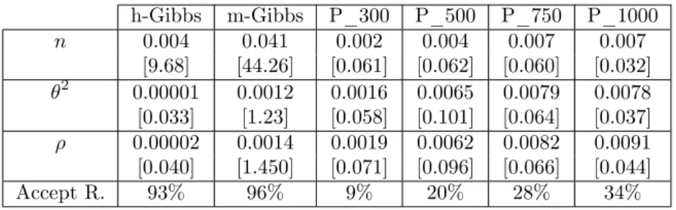
The ESS of the PMMH depends on the number of particles used in the bootstrap …lter. Table 3 shows that when considering computation time choosing 50 particles gives better results (although fornchoosing 25 particles gives slightly better results). However, the m-Gibbs sampler is 4.7 times better than the best PMMH in terms of ESS/TIME to sample n, whereas the improvements for and 2 are 62% and 9.4%, respectively. When we compare the m-Gibbs with the h-Gibbs, we can see that the m-Gibbs is between 4.9 and 6.2 times more e¢ cient.
In Table 4 we can see that choosing 500 or 1000 particles gives roughly the same ESS for the PMMH, indicating that there is not much further gain in increasing the number of particles. Thus we can expect that the PMMH algorithm with 1000 particles has practically the same ESS as the ideal algorithm that samples marginally on the volatilities (Andrieu et al. (2010)). Thus it is interesting to compare the ESS sample size of the m-Gibbs and the h-Gibbs with the ESS of such ideal algorithm. In Table 4 we can see that the m-Gibbs has roughly the same ESS fornas the ideal algorithm, but the ESS for 2and is 15% and 22.6%, respectively, of the ideal algorithm. Because the number of observations is relatively small and the prior for is quite spread, the 95% posterior credible interval for is wide and equal to(0:76;0:98). Although not shown in the tables, all algorithms produced the same summary of the posterior distribution, indicating the absence of programming errors. Overall Tables 3 and 4 show that the m-Gibbs algorithm is much more e¢ cient than the best PMMH even whenT is as small as 100 and much more e¢ cient also than the h-Gibbs.
h-Gibbs m-Gibbs P_25 P_50 P_100 P_500 P_1000 n 0.0037 0.0302 0.0113 0.015 0.021 0.042 0.028 [150.3] [730.6] [155.9] [122.9] [83.5] [14.9] [2.8] 2 0.0011 0.0105 0.015 0.029 0.034 0.063 0.069 [46.1] [253.2] [201.9] [231.3] [134.5] [22.4] [6.8] 0.0015 0.015 0.016 0.029 0.034 0.06 0.07 [60.1] [372.8] [219.3] [230.1] [137.5] [21.9] [6.8] Accept R. 93% 93% 21% 34% 45% 50% 52%
Table 3: E¤ective Sample Size (ESS) and ESS over time (ESS/TIME) for the h-Gibbs, the m-Gibbs and PMMH algorithms using 100 arti…cial observations. ESS/TIME is in squared brackets and represents the number of independent samples per minute. The column P_25 refers to the PMMH algorithm that uses 25 particles. The row Accept R. gives the acceptance rate in the Metropolis step. Note that in the h-Gibbs and m-Gibbs the Metropolis step is repeated 10 times, and Accept R. is the probability of accepting a new value in the sequence of 10 draws.
h-Gibbs m-Gibbs P_25 P_50 P_100 P_500 P_1000
n 13.1 107.7 40.3 54.9 74.2 149.2 100
2 1.6 15.3 21.4 42.3 49.0 91.9 100
2.2 22.6 23.3 42.3 50.3 90.2 100
Table 4: E¤ective Sample Size (ESS) as a proportion of the ESS of the PMMH with 1000 particles.
Let us now compare the e¢ ciency of the algorithms using 2000 daily observations of the exchange rate Yen - US dollar (6th Aug 2003 - 15th Jul. 2011). ytis the …rst di¤erence of the log exchange rate andxt 1
includes a constant and a lag, so that = ( 0; 1). In Table 5 we can see that it is best to choose 500 particles for the PMMH and that the m-Gibbs is 710 times more e¢ cient than the best PMMH to sample
n, 15 times more e¢ cient to sample and 12 times more e¢ cient to sample 2. With respect to the h-Gibbs algorithm, the m-Gibbs is about 36 times more e¢ cient to sample 2 or and 4.6 times more e¢ cient to samplen. The posterior 95% credible interval for is (0:956;0:99), which is quite close to 1. That is one reason why the relative performance of the h-Gibbs is particularly bad in this case.
h-Gibbs m-Gibbs P_300 P_500 P_750 P_1000 n 0.004 0.041 0.002 0.004 0.007 0.007 [9.68] [44.26] [0.061] [0.062] [0.060] [0.032] 2 0.00001 0.0012 0.0016 0.0065 0.0079 0.0078 [0.033] [1.23] [0.058] [0.101] [0.064] [0.037] 0.00002 0.0014 0.0019 0.0062 0.0082 0.0091 [0.040] [1.450] [0.071] [0.096] [0.066] [0.044] Accept R. 93% 96% 9% 20% 28% 34%
Table 5: E¤ective Sample Size (ESS) and ESS over time (ESS/TIME) for the h-Gibbs, the m-Gibbs and PMMH algorithms using 2000 observations of the US-Japan exchange rate. ESS/TIME is in squared brack-ets and represents the number of independent samples per minute. See explanation in Table 3 for other de…nitions.
5
Empirical Application
The aim of this section is to compare the empirical performance of several models using real macroeconomic and …nancial data. In addition to the ARG and FTARG described in Section 2, we consider the model where
2
t follows a log-normal distribution (LNORM) (using the SvPack in Ox provided by Kim et al (1998)). In addition, we consider 3 models whereetfollows a student-t distribution: ARG-T, FTARG-T and LNORM-T. These 3 models are the same as the ARG, FTARG and LNORM models, respectively, but assume a student-t distribution foret instead of normal. We run the models separately on 4 datasets, 3 of which are exchange rates (1 daily exchange rate and 2 monthly) and one dataset corresponds to UK in‡ation (see Table 6 for more details on the data). The dependent variableytis either the level of in‡ation or the …rst di¤erence of the log exchange rate. When yt is the return of the exchange rate, xt contains a constant and a lag of yt. Whenyt is in‡ation, xt contains a constant, two lags of in‡ation, the unemployment rate and two lags of the unemployment rate (as in the estimation of a Phillips curve, e.g. Staiger et al. (1997) or Sargent et al. (2006)). The exchange rate data was obtained from the Federal Reserve Bank of St. Louis, and the in‡ation and unemployment rate data from OECD (2010).
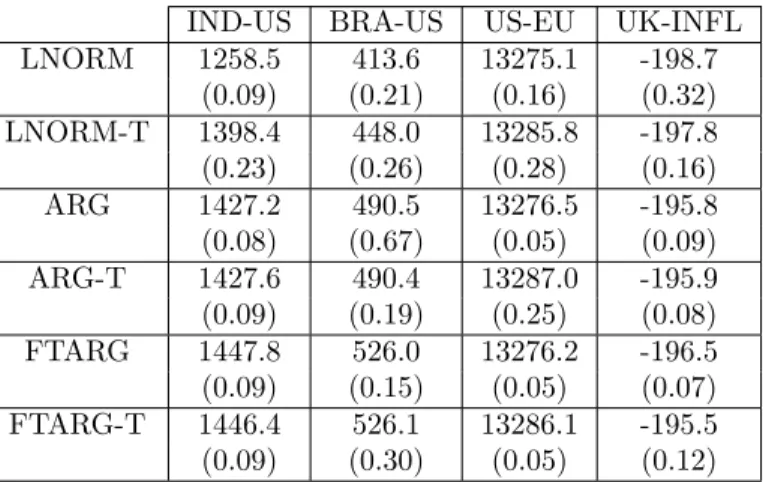
Table 7 shows the value of the log-likelihood at the posterior median of parameters, calculated using the bootstrap particle …lter (e.g. Gordon et al. (1993)), and using the prior speci…cation shown in the appendix. Marginal likelihood values (calculated with the method of Chib and Jeliazkov, (2001)), show a similar patter and are given in Table 8. We can see that the ARG model has a much higher value of the log likelihood than the LNORM and LNORM-T models for the monthly India-US and Brazil-US exchange rates. The improvement in the log-likelihood is as much as 30 (India-US) or 40 (Brazil-US) points over the LNORM-T. Furthermore, for these two exchange rates the FTARG model is much superior than all the other simpler models (by more than 20 points or 36 points increase in the log likelihood with respect to the ARG). The extension to student-t errors does not bring any noticeable improvement in the value of the log-likelihood of the ARG or FTARG models, although it does increase the log likelihood of the LNORM model. In summary, the FTARG is a clear winner in the case of the monthly India-US and Brazil-US exchange rates.
Regarding the EU-US exchange rate, the LNORM-T and ARG-T are substantially better than the LNORM and ARG, again indicating that it is important to allow for student-t errors. Both the LNORM-T and the ARG-T seem to perform equally well, whereas the FTARG and FTARG-T models do not bring any noticeable increase in the log likelihood. Hence, the LNORM-T and ARG-T could be said to be joint winners for the EU-US exchange rate, as con…rmed by the marginal likelihood values in Table 8.
Finally, regarding the estimation of the Phillips curve for UK in‡ation, all models have very similar values for the log likelihood, indicating that the simpler models (LNORM and ARG) might be more adequate in
IND-US Exchange rate Indian Rupee - US dollar, monthly average: March 1973 - June 2013, 484 observations
BRA-US Exchange rate Brazilian Real - US dollar, monthly average: March 1995 - June 2013, 220 observations
EU-US Exchange rate Euro - US dollar, daily: 6 Jan 1999 - 17 May 2013, 3615 observations
UK-INFL Quarterly In‡ation based on GDP de‡ator, seasonally adjusted, 1971Q1 - 2011Q4, 162 observations.
UK-UR
Harmonized Unemployment Rate: All Persons for United Kingdom, seasonally adjusted, 1971Q1 - 2011Q4, 162
observations.
Table 6: Description of variables used in empirical analysis
IND-US BRA-US US-EU UK-INFL
LNORM 1258.5 413.6 13275.1 -198.7 (0.09) (0.21) (0.16) (0.32) LNORM-T 1398.4 448.0 13285.8 -197.8 (0.23) (0.26) (0.28) (0.16) ARG 1427.2 490.5 13276.5 -195.8 (0.08) (0.67) (0.05) (0.09) ARG-T 1427.6 490.4 13287.0 -195.9 (0.09) (0.19) (0.25) (0.08) FTARG 1447.8 526.0 13276.2 -196.5 (0.09) (0.15) (0.05) (0.07) FTARG-T 1446.4 526.1 13286.1 -195.5 (0.09) (0.30) (0.05) (0.12)
Table 7: Value of Log-Likelihood at the posterior median, calculated with a particle …lter for di¤erent models and datasets. Numerical standard error in brackets (obtained using independent estimates of the likelihood).
the estimation of the Phillips curve with UK data.
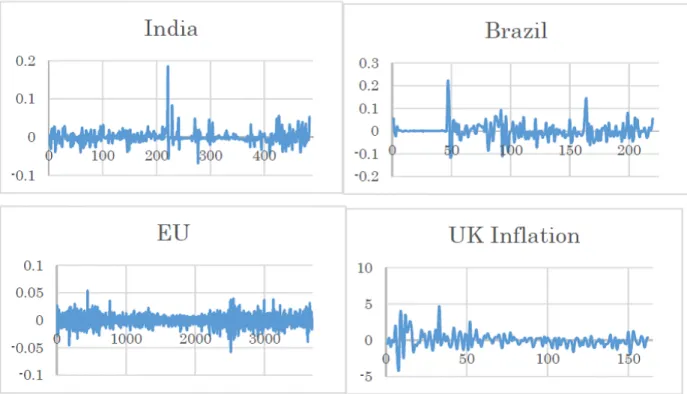
Figure 4 shows the OLS residuals for each of the 5 datasets. We can observe larger jumps in volatility in the exchange rates of India and Brazil, which might be one of the reasons why the inverse gamma models perform much better than the log-normal models in these datasets. Another reason might be that inverse gamma models allow for greater correlation in the volatility outliers than the LNORM-T model. To see this recall that the LNORM-T model can be written as a mixture of normals: yt = xt +et, where
et N(0; t1 2t)and tare i.i.d. draws from a gamma distribution. Therefore the volatility ofet has two components, one determined by 2
t and another by t. Because thas no serial correlation, the LNORM-T model does not allow for persistence in the volatility outliers. This is not so in the inverse gamma and generalized inverse gamma models, where the volatility ofethas only one component 2t, which has positive correlation with 2t 1regardless of whether 2t 1was on the tail of the distribution or not.
IND-US BRA-US US-EU UK-INFL LNORM 1259.1 390.7 13236.1 -236.7 (0.45) (0.21) (0.16) (0.32) LNORM-T 1365.2 421.5 13247.2 -231.9 (0.23) (0.26) (0.28) (0.16) ARG 1401.0 467.3 13241.0 -256.1 (0.08) (0.67) (0.05) (0.09) ARG-T 1401.1 466.9 13249.8 -255.5 (0.09) (0.19) (0.25) (0.07) FTARG 1426.0 497.0 13234.5 -260.1 (0.12) (0.19) (0.05) (0.09) FTARG-T 1419.6 494.0 13242.2 -263.5 (0.09) (0.33) (0.05) (0.12)
Table 8: Value of Marginal Likelihood calculated using the method of Chib and Jeliazkov (2001), but the posterior ordinate for (n; 2, , V, $) was calculated using a normal approximation. Numerical standard error in brackets.
Figure 4: OLS residuals for 4 di¤erent datasets: 3 exchange rates versus the US dollar and a Phillips Curve for UK in‡ation.
6
Conclusions
This paper has developed e¢ cient posterior simulators for inverse gamma and generalized inverse gamma processes for stochastic volatility. By conditioning on some auxiliary variables, it is shown that it is possible to draw all the volatilities jointly using simple distributions such as Poisson and Gamma. Furthermore, the unknown parameters can be drawn after integrating out the volatilities. Estimations with real and simulated data show that the new algorithm is much more e¢ cient than the recently developed Particle MCMC algorithms that generate the volatilities and unknown parameters in a joint move.
We also developed a new type of generalized inverse gamma time-series model and analytically derived its properties. Using simulation we calculated the percentiles of the distribution and illustrated that the generalized inverse gamma process has much greater ‡exibility in the right tail. In this way we provide a new class of ‡exible stochastic volatility models that can be estimated with simple and e¢ cient MCMC algorithms. Furthermore, the FTARG process can be further generalized by specifying Tet to be a mixture of beta distributions, since such a mixture can approximate any distribution in the interval (0;1). Finally, the empirical exercise shows that inverse gamma and generalized inverse gamma models outperform the lognormal volatility model with student-t errors specially in the datasets that exhibit greater jumps and correlation of volatility outliers, such as the exchange rates of Brazil-US or India-US.
References:
Abraham, B., N. Balakrishna and R. Sivakumar (2006) "Gamma Stochastic Volatility Models" Journal of Forecasting, 25, 153–171.
Andrieu, C., A. Doucet, and R. Holenstein, (2010), "Particle Markov chain Monte Carlo methods,"Journal of the Royal Statistical Society: Series B (Statistical Methodology), 72, 269–342.
Asai, M. (2005) "Comparison of MCMC Methods for Estimating Stochastic Volatility Models,"Computational Economics, 25, 281-301.
Barndor¤-Neilsen, O. E. and N. Shephard (2001) "Non-Gaussian Ornstein-Ulhlenbeck-based models and some of their uses in …nancial economics"Journal of the Royal Statistical Society, Series B, 63, 167–241. Bauwens, L., M. Lubrano, and J.F. Richard (1999)Bayesian Inference in Dynamic Econometric Models. Oxford: Oxford University Press.
Casarin, R. and D. Sartore, (2007), "Matrix-state particle …lters for Wishart stochastic volatility processes," inProceedings SIS, 2007 Intermediate Conference, Risk and Prediction, 399-409, CLEUP Padova.
Chib, S., I. Jeliazkov (2001) "Marginal Likelihood From the Metropolis–Hastings Output," Journal of the American Statistical Association,96, 270-281.
Chib, S., F. Nardarib and N. Shephard (2002) "Markov Chain Monte Carlo Methods for Stochastic Volatility Models,"Journal of Econometrics, 108, 281 –316.
Creal, D. (2013) "A Class of Non-Gaussian State Space Models with Exact Likelihood Inference," Available at SSRN: http://ssrn.com/abstract=2310256 or http://dx.doi.org/10.2139/ssrn.2310256
Delatola, E.I. and J.E. Gri¢ n (2011) "Bayesian nonparametric modelling of the return distribution with stochastic volatilty"Bayesian Analysis 6, 1–26.
Devroye, L. (2002) "Simulating Bessel Random Variables,"Statistics & Probability Letters, 57, 249–257. Dubey, S. D. (1970) "Compound Gamma, beta and F distributions,"Metrika, 16, 27-31.
Durham, G.B. (2007) "SV mixture models with application to S&P 500 index return,"Journal of Financial Economics,85, 822–856.
Fox, E.B. and M. West (2011) "Autoregressive Models for Variance Matrices: Stationary Inverse Wishart Processes" arXiv:1107.5239.
Frühwirth-Schnatter, S. and L. Sögner (2009) "Bayesian estimation of stochastic volatility models based on OU processes with marginal Gamma law,"Annals of the Institute of Statistical Mathematics, 61, 159–179. Gelman, A., G.O. Roberts and W.R. Gilks (1996) “E¢ cient Metropolis Jumping Rules,”inBayesian Statistics
5, eds. J. M. Bernardo, J. O. Berger, A. P. Dawid, and A. F. M. Smith, Oxford, U.K.: Oxford University Press, pp. 599–608.
Gordon, N., D. Salmond and A.F.M. Smith, (1993) "Novel approach to nonlinear and non-Gaussian Bayesian state estimation,"Proc. Inst. Elect. Eng., F., 140, 107-113.
Gourieroux, C. and J. Jasiak (2006) "Autoregressive Gamma Processes"Journal of Forecasting, 129–152. Gourieroux, C., J. Jasiak and R. Sufana (2009) "The Wishart Autoregressive process of multivariate sto-chastic volatility,"Journal of Econometrics, 150, 167 - 181.
Gri¢ n, J. E. and M.F.J. Steel, (2006a) "Inference with non-Gaussian Ornstein-Uhlenbeck processes for stochastic volatility,"Journal of Econometrics, 134, 605–644.
Gri¢ n, J.E. and M.F.J. Steel (2006b) "Ordered-based dependent Dirichlet processes,"Journal of the American Statistical Association,101, 179–194.
Gri¢ n, J.E. and M.F.J. Steel (2011) "Stick-breaking autoregressive processes,"Journal of Econometrics,162, 383–396.
Iliopoulos, G. and D. Karlis (2003) "Simulation from the bessel distribution with applications,"Journal of Statistical Computation and Simulation, 73:7, 491-506.
Jacquier, E., N. G. Polson, and P. E. Rossi (1994). "Bayesian analysis of stochastic volatility models (with discussion)"Journal of Business and Economic Statistics,12, 371 - 389.
Janssen, A and H. Drees (2013) "A stochastic volatility model with ‡exible extremal dependence structure,"
arXiv.org, arXiv:1310.4621v1.
Jensen, M.J. and J.M. Maheu (2010) "Bayesian semiparametric stochastic volatility modeling", Journal of Econometrics,157, 306–316.
Jensen, M.J. and J.M. Maheu (2014)."Estimating a semiparametric asymmetric stochastic volatility model with a Dirichlet process mixture,"Journal of Econometrics, 178, 523-538.
Johnson, N.L., S. Kotz and N. Balakrishnan (1994),Continuous Univariate Distributions, Volume 1, 2ndEdition,
John Wiley & Sons, Inc.
Johnson, N.L., S. Kotz and N. Balakrishnan (1995),Continuous Univariate Distributions, Volume 2, 2ndEdition,
John Wiley & Sons, Inc.
Johnson, N.L., A.W. Kemp and S. Kotz (2005),Univariate Discrete Distributions, 3rd Edition, John Wiley &
Sons, Inc.
Kachitvichyanukul, V. and B.M. Schmeiser (1988) "Algorithm 668: H2PEC: sampling from the hypergeo-metric distribution,"ACM Transactions on.Mathematical Software, 14, 397-398.
Kim, S., N. Shephard, and S. Chib (1998) "Stochastic Volatility: Likelihood Inference and Comparison with ARCH Models,"The Review of Economic Studies, 65, 361-393.
Koop, G. (2003)Bayesian Econometrics, Wiley.
Krishnaiah, P. and M. Rao (1961), "Remarks on a multivariate Gamma distribution,"The American Mathe-matical Monthly, 68, 342-346.
Monahan, J.F. (2001),Numerical Methods of Statistics, Volume 1, Cambridge University Press.
OECD (2010), "Main Economic Indicators - complete database", Main Economic Indicators (database), http://dx.doi.org/10.1787/data-00052-en (Accessed on Feb 2014)
Philipov, A. and M. E. Glickman (2006) "Multivariate stochastic volatility via Wishart processes,"Journal of Business and Economic Statistics 24, 313–328.
Roberts, G. O., O. Papaspiliopoulos and P. Dellaportas, (2004) "Bayesian inference for non-Gaussian Ornstein-Uhlenbeck stochastic volatility processes"Journal of Royal Statistical Society, Series B, 66, 369–393. Sargent, T.,N. Williams, and T. Zha, (2006), “Shocks and Government Beliefs: The Rise and Fall of American In‡ation,”American Economic Review, 96, 1193–1224.
Shephard, N. and M. K. Pitt (1997). "Likelihood analysis of non-Gaussian measurement time series" Bio-metrika 84, 653–667.
Sims, C. and Zha, T., 2006. Were there regime switches in macroeconomic policy? American Economic Review
96, 54-81.
Stacy, E. W. (1962) "A Generalization of the Gamma Distribution," Annals of Mathematical Statistics, 33, 1187-1192.
Stadlober, E (1989) "The Ratio of Uniforms Approach for Generating Discrete Random Variables,"Journal of Computational and Applied Mathematics, 31, 181-189.
Staiger, D., J. Stock and M. Watson (1997), “The NAIRU, Unemployment and Monetary Policy,”Journal of Economic Perspectives, 11, 33–49.
Steel, M. (1998) "Bayesian Analysis of Stochastic Volatility Models with Flexible Tails,"Econometric Reviews, 17, 109-143.
Triantafyllopoulos, K. (2010) "Multi-variate stochastic volatility modelling using Wishart autoregressive processes"Journal of Time Series Analysis, 33, 48-60.
Watanabe, T. and Y. Omori (2004) "A multi-move sampler for estimating non-Gaussian times series models: Comments on Shephard and Pitt (1997)"Biometrika 91, 246–248.
Winkelmann, R. (2008) Econometric Analysis of Count Data, Springer.
Yuan, L. and J.D. Kalb‡eisch (2000) "On the Bessel distribution and related problems" Ann. Inst. Statist. Math., 52, 438–447.
Appendix
Prior Speci…cation in the Empirical Application
For the Gamma type models we speci…ed the prior as: ln(n) N(ln(40);1:5), 2
B(8;1), 2
G(1;200),
ln(V) N(ln(20);1).
For the log-normal volatility model we use the same prior speci…cation and the same notation as in Kim, Shephard and Chib (1998): N(0;10); 2 1
G(2:5;40),( + 1)=2 B(20;1:5).
In all models the prior for isN(0; T I), whereI is the identity matrix andT is the sample size.
For the models with student-t errors, we specifyln($) N(ln(40);1:5), where$ is the parameter for the degrees of freedom of the student-t.
For some datasets the log-normal volatility model did not converge with the baseline prior, and in those cases we used a tighter prior for 2
to ensure convergence: 2 1
G(17:5;57:14) (Brazil), 2 1
G(22:5;444:4) (India, normal errors), 2 1
G(17:5;57:14) (India, student-t errors), 2 1
G(3:5;28:57)
(UK in‡ation).
As mentioned above, in the Metropolis step we target the conditional posterior of = ( 1; 2; 3), de…ned
as: 1 = ln(n) + ln( 2) ln(1 2), 2 = ln( 2) and 3 = ln(1 2). The inverse transformation is ( ) =
(n( ); 2( ); 2( )) = (exp(
1 2 3);exp( 2);1 exp( 3)). Since our prior is de…ned on = (ln(n); 2; 2),
the prior of can be written using the Jacobian as: p( ) 2(1 2), where p( ) is the prior of and
[ 2(1 2)] is the Jacobian of the transformation.
In the FTARG model instead of specifying the prior on( 2, 2
)we specify it on(e2,e2), and the Metropolis step targets the conditional posterior of 1= ln(n) + ln(e
2
) ln(1 e2), 2= ln(e 2
)and 3= ln(1 e2).
Proof of Proposition 1
From equation (2) we can write the process forzt as:
zt= q e Tt"t+ q e Tt q e Tt 1"t 1+ 2 q e Tt q e Tt 1 q e Tt 2"t 2+ 3 q e Tt q e Tt 1 q e Tt 2 q e Tt 3"t 3+:::
which implies that the stationary distribution ofztjTeisN(0; 2vc;t)and so the stationary distribution ofkt is
that of the product ofvc;tand"0t"t. Hence the moments ofkt can be calculated asE(kts) =E(v s
c;t)E(("0t"t) s
). Because("0t"t) is distributed as aG(n=2;2 2), its moments are given by (e.g. Johnson et al. (1994 p. 339)):
E( "0t"t s ) = 2 s sY1 i=0 (n+ 2i) To calculate E(vs
c;t) note that we can write vc;t as vc;t = Tet + 2Tetvc;(t 1). so that E(vsc;t) = E((Tet+
2Te
E((Tet+ 2Tetvc;(t 1))s) =E(Tets) s X i=0 s i ! 2i E(vic;(t 1)) (19)
Because E(vsc;t) = E(vsc;(t 1)), (19) implies property (10) and the other unconditional moments stated in
Proposition 1. To obtain the conditional moments, note that equation (3) can be written as:
kt= e
Tt
E(Tet)
(e2kt 1+e"0te"t+ 2ee"0tzt 1) (20)
Becausee"t is independent ofzt 1 and E(e"t) = 0we obtain thatE(e"0tzt 1) = 0. Taking into account that
E(e"0te"t) =ne
2
we can take conditional expectations on both sides of (20) to get equations (4) and (7). Let us calculatecov(kt; kt h)ascov(kt; kt h) =E(ktkt h) [E(kt)]2. To deriveE(ktkt h)let us use iterative
expectations to rewrite equation (4) as:
E(ktjkt h) =e2hkt h+ h 1
X i=0
e2i(1 e2)E(kt) (21)
Multiplying both sides of (21) bykt hand then taking expectations with respect tokt hwe obtain:
E(ktkt h) =e2hE(k2t h) + h 1 X i=0 e2i (1 e2) [E(kt)]2=e2hE(kt2 h) + (1 e 2h ) [E(kt)]2
where we have used the formula for the sum of a geometric series. Thuscov(kt; kt h) =E(ktkt h) [E(kt)]2= e2h
(E(k2t h) [E(kt)]2) =e2hvar(kt). Thus, the correlation betweenkt andkt hise2h.
Because the stationary distribution of 2
t = 1=ktis that of the product of(vc;t) 1and("0t"t)
1
, with(vc;t) 1
being independent of("0t"t) 1, the expectationE( 2ts) is …nite if and only if bothE((vc;t) s) andE(("0t"t) s)
are …nite. Because ("0t"t) 1 is an inverted gamma with n degrees of freedom, E(("0t"t) s) is …nite only if
2s < n. In addition, fromvc;t=Tet(1 + 2vc;(t 1))it follows that:
1 vc;t = 1 e Tt 1 1 + 2v c;(t 1) Because (1 + 2v
c;(t 1)) s <1, it follows that E((1 + 2vc;(t 1)) s) is …nite because the density function of
vc;(t 1) integrates up to 1. BecauseTet follows aB( ; ), E(Tet s) is …nite if and only if > s. Putting both
conditions together,E( 2ts)is …nite when > sandn >2s.
For the ARG model (i.e. Tet= 1for all t), the expressions for the expected value and variance of 2t are
calculate the correlations between 2
t and
2
t s in the ARG model, let us …rst proof the following property:
E( 2tj 2 t s) = Z Ys i=2 (ui)n=2 ! 1 2 (n 2)exp (1 us) 2 2 2 1 2 t s p(u1)du1 (22)
where u1 B((n 2)=2;1), p(u1) is the density function ofu1 and us = 1=(1 + 2(1 us 1)) for s 2.
To proof this note that the Poisson representation in (11) implies that ktj(kt 1; ht) is a Gamma which in
turn implies that 2
tj( 2t 1; ht) is anIG2( 2; n+ 2ht), such thatE( 2tj( 2t 1; ht)) = 2=(n+ 2ht 2). We can
therefore integrate outht to obtainE( 2tj 2t 1).as:
E( 2tj 2 t 1) = 1 2exp( t) 1 X i=0 i t i! 1 n+ 2i 2 , where t= 2 2 2 t 1 2 (23)
Note that1=(n+ 2i 2) = (n 2) 1[n=2 1]i=[n=2]i= (n 2) 1E((u1)i), where[n=2]i is the rising factorial.
Therefore (23) can be written as:
E( 2tj 2 t 1) = Z 1 2 exp( t) 1 (n 2) 1 X i=0 i t i! (u1) i p(u1)du1= (24) Z 1 2exp( t) 1 (n 2)exp( tu1)p(u1)du1 Z 1 2 1 (n 2)exp (1 u1) 2 2 2 1 2 t 1 p(u1)du1
which is the same as (22) for the case s = 1. To proof (22) for s = 2 we need to integrate E( 2tj 2t 1)
with respect to p( 2t 1j 2t 2) using expression (24). This can be done by …rst integrating with respect to
p( 2
t 1jht 1; 2t 2) (which is a IG2( 2; n+ 2ht 1)) and then integrating out ht 1 (using a P( t 1)). The
proof for s > 2 can be obtained by repeating the same process, that is, integrate out with respect to
p( 2
t s+1jht s+1; 2t s) and then integrate outht s+1 (using aP( t s+1)).
E( 2
t 2t s) can be obtained by using expression (22) to calculate E( t2 2t sj 2t s) and then integrate out
2
t s using the stationary distribution IG2( 2; n). This gives:
E( 2t 2t s) = (1 2)n=2 2 2 2(n=2 1)2 Z Ys i=2 (ui)n=2 ! 1 1 2u s n=2 1 p(u1)du1 (25)
By using the de…nition ofus it is possible to verify that:
s Y i=2 ui ! 1 1 2u s = sY1 i=2 ui ! us 1 2u s = sY1 i=2 ui ! 1 1 2u s 1 = 1 1 2u 1
and: s Y i=2 ui=usus 1 sY2 i=2 ui= 1 1 + ( 2+ 4)(1 u s 2) sY2 i=2 ui= 1 1 + 2 s(1 u1) where 2 s= Ps g=1 2g
. Hence, the integral in expression (25) can be written as:
E " Ys i=2 (ui)n=2 ! 1 1 2u s n=2 1# = E " 1 1 + 2 s(1 u1) 1 1 2u 1 n=2 1# = (26) 1 1 + 2 s E " 1 1 b2su1 1 1 2u 1 n=2 1#
where the expectation is calculated with respect tou1 andb2s =
2 s=(1 + 2 s). By expanding(1=(1 2 u1))n=2 1
as a hypergeometric series (e.g. Muirhead (1985, p. 259)) and using basic properties of the beta distribution, it is possible to show that:
E " (uh1) 1 1 2u 1 n=2 1# = [n=2 1]h [n=2]h 2F1( n 2 1; n 2 1 +h; n 2+h; 2 )
and therefore the expectation in (26) can be written as:
1 1 + 2 s 1 X h=0 b2 s h [n=2 1]h [n=2]h 2F1( n 2 1; n 2 1 +h; n 2+h; 2 ) = 1 1 + 2 s 1 X h=0 1 X i=0 " b2 s h 2 i h!i! [1]h [n=2 1]h+i [n=2]h+i [n=2 1]i # = 1 1 + 2 s F1 hn 2 1; 1; n 2 1; n 2;b 2 s; 2i
whereF1[:]is an Appell series of the …rst type (e.g. Slater (1966, p. 210)), which in our case can be reduced
to a2F1(:)series (Slater (1966, p. 219)): F1 hn 2 1; 1; n 2 1; n 2;b 2 s; 2i = 1 1 2 n=2 1 2F1 n 2 1;1; n 2; b2 s 2 1 2 = 1 1 2 n=2 1 2F1 n 2 1;1; n 2; 2s 1 2s
Using the Euler relationships (e.g. Muirhead (1982, p. 265) ), the2F1(:)series can be written as:
2F1 n 2 1;1; n 2; 2s 1 2s = (1 2s )h2F1 1;1; n 2; 2s i
Putting all this together the expectation in (26) can be written as: E " Ys i=2 (ui)n=2 ! 1 1 2u s n=2 1# = 1 2s 1 + 2 s 1 1 2 n=2 1h 2F1 1;1; n 2; 2s i = (1 2) 1 1 2 n=2 1h 2F1 1;1; n 2; 2s i
where we have used that a geometric series can be written as1 + 2
s = (1
2s)=(1 2). This proves that
(25) is equal to: E( 2t 2t s) = (1 2)2 2 2 2(n=2 1)2 h 2F1 1;1; n 2; 2s i
The correlation corr( 2t; 2t s) can then be calculated as E( 2t 2t s) E( 2t) =var( t2), where E( 2t) and
var( 2t) are obtained from the properties of the inverted gamma distribution (e.g. Bauwens et al. (1999.
p.292)).
Proof of Proposition 2
The likelihood is:
L(Yjk; ) = (2 ) T =2 "T Y t=1 (kt)1=2 # exp 1 2 T X t=1 r2tkt ! r2t = (yt xt )2
The prior p(k; hj ; )is equal to:
p(k1j ; ) T Y t=2 (p(ktjht; ; )p(htjkt 1; ; )) = p(k1j ; ) T Y t=2 0 @p(ktjht; ; ) ht t ht! exp( t) 1 A
The densities p(k1j ; )andp(ktjht; ; )are Gamma densities:
p(k1j ; ) = j k1j n 2 2 c1 exp 1 e 2 2e2 k1 c1= n 2 2e2 1 e2 !n=2 (27) p(ktjht; ; ) = j ktj n+2ht 2 2 ct exp 1 2e2t kt ! ct= n 2 +ht 2e 2 t n=2+ht t= 2; :::; T
Thus, the product of the prior and the likelihood,p( ; )p(k; hj ; )L(Yjk; ), can be written as: (2 ) T =2 "YT t=1 (kt) n+2ht 2 2 +12 # exp 1 2 T X t=2 kt 1 e2 t +r2t !! (28) exp 1 2k1 1 e2 e2 +r 2 t T Y t=2 0 @ ht t ht! exp( t) 1 A T Y t=1 ct ! 1 p( ) Recalling that t=e2tkt 1=(2e 2
t)and also that(e2t=e
2
t) = (e2t+1=e 2
t+1), it is clear thatktjh; ; G((n+ 1)=2 +
ht+ht+1;2re2t). To …nd the conditional distribution of h given k note that ct depends on ht and putting
together the terms in (28) that depend onht we get:
T Y t=2 0 @ 1 ht! 1 (n=2 +ht) et 2e2t !2 ktkt 1 !ht1 A
which shows thathtjk; ; Bessel(n22;et
pk tkt 1
e2 t
) for t= 2:::T. The expression for p(n; 2; 2
jY; h; )can be obtained by integrating (28) with respect tok using basic properties of the Gamma distribution.
Proof of Proposition 3:
For the proof let us write the hypergeometric distribution in (15) using the gamma function and the factorial instead of the binomial coe¢ cients, so thatPr (dt=sjht; dt+1) is equal to:
ht! dt!(ht dt)! ((n+ 1)=2 +dt+1) ((n 1)=2 +dt) (2 +dt+1) (2 +dt+1 dt) ((n 1)=2 +ht) ((n+ 1)=2 +dt+1+ht)
Thus, the joint prior of(d= (d2; :::; dT))given(h; k; m), denoted as (djh; k; m);can be written as:
(djh; k; m) =
2
Y t=T
p(dtjht; dt+1) with dT+1= 0
and we will also use the notationp(d2:T ljdT l+1; h; k; m)for:
p(d2:T ljdT l+1; h; k; m) = 2
Y t=T l
p(dtjht; dt+1)
p(k1j ; ) T Y t=2 (p(ktjht; ; )p(mtjht)p(htjkt 1; ; )) = p(k1j ; ) T Y t=2 0 @p(ktjht; ; ) ht t ht!m ht t exp( t) ( m+ m+ht) ( m+ht) ( m) m m 1 t (1 mt) m 1 1 A
wherep(k1j ; )andp(ktjht; ; )have been de…ned in (27), and where m= (n 1)=2, m= 1=2, as de…ned
before.
Thus, the product of the prior and the likelihood,p(k; h; m; dj ; )L(Yjk; ), can be written as:
(2 ) T =2 "YT t=1 (kt) n+2ht 2 2 + 1 2 # exp 1 2 T X t=2 kt 1 e2 t +r2t ! 1 2k1 1 e2 e2 +r 2 1 ! T Y t=2 0 @ ht t ht!m ht t exp( t) (n=2 +ht) ((n 1)=2 +ht) ( m) m m 1 t (1 mt) m 1 1 A (djh; k; m) T Y t=1 ct ! 1
It is clear that the conditional posterior ofkTjhT; m; dis aG((n+ 1)=2 +hT;2rb2T). Integrating outkT we …nd:
((n+ 1)=2 +hT) 2br2T n+1+2hT 2 (2 ) T =2 "T 1 Y t=1 (kt) n+2ht 2 2 + 1 2 # (29) exp 1 2 TX1 t=2 kt 1 e2 +r 2 t 1 2k1 1 e2 e2 +r 2 1 ! T Y t=2 0 @ ht t ht!m ht t exp( t) (n=2 +ht) ((n 1)=2 +ht) ( m) m m 1 t (1 mt) m 1 1 Ap(djh; k; m) T Y t=1 ct ! 1
In order to …nd out the posterior conditional ofhT, note that cT depends onhT and so the terms that
containhT in expression (29) can be written as:
((n+ 1)=2 +hT) 2br2T hT hT T hT! mhT T (n=2 +hT) ((n 1)=2 +hT) (30) 2e2T hT (n=2 +hT) hT! (hT dT)! ((n 1)=2 +hT) ((n+ 1)=2 +dT+1+hT) = bT hT 1 (hT dT)!
where we have implicitly used that: bT= T mTrb2T e2 T ! anddT+1= 0
Recall that the restriction dT hT comes from the prior ofdT. Therefore (30) implies thathTjkT 1; m; d
is aSP(bT; dT). Summing up expression (30) over all values of hT 2[dT;1) gives bT dT
exp(bT). Thus,
integrating outhT from (29) we obtain:
bT dT exp ( T bT) (31) 2brT2 n+1 2 (2 ) T =2 "T 1 Y t=1 (kt) n+2ht 2 2 +12 # exp 1 2 TX1 t=2 kt 1 e2 t +r2t ! 1 2k1 1 e2 e2 +r 2 1 ! TY1 t=2 0 @ ht t ht!m ht t exp( t) (n=2 +ht) ((n 1)=2 +ht) 1 A T Y t=2 1 ( m)m m 1 t (1 mt) m 1 1 dT! ((n+ 1)=2) ((n 1)=2 +dT) (2) (2 dT) 2e2T n=2 p(d2:T 1jdT; h; k; m) TY1 t=1 ct ! 1 Noting that: exp ( T bT) = exp 1 2 e2 T e2 T mT eT e2 T !2 b r2T ! kT 1 ! we obtain that: exp 1 2kT 1 1 e2 T 1 +r2T 1 !! exp ( T bT) = exp 1 2br2 T 1 kT 1
Therefore the conditional posteriorkT 1jhT 1; m; dis aG((n+ 1)=2 +dT+hT 1;2brT2 1). Thus, integrating out
2br2T n+1 2 2 b r2T 1 n+1 2 +hT 1+dT ((n+ 1)=2 +dT+hT 1) (32) mT 2 eT e2 T !2 b rT2 !dT (2 ) T =2 "TY2 t=1 (kt) n+2ht 2 2 +12 # exp 1 2 TX2 t=2 kt 1 e2 t +rt2 ! 1 2k1 1 e2 e2 +r 2 1 ! TY1 t=2 0 @ ht t ht!m ht t exp( t) (n=2 +ht) ((n 1)=2 +ht) 1 A T Y t=2 1 ( m)m m 1 t (1 mt) m 1 1 dT! ((n+ 1)=2) ((n 1)=2 +dT) (2) (2 dT) 2e2T n=2 p(d2:T 1jdT; h; k; m) TY1 t=1 ct ! 1
The terms that depend on hT 1 are:
((n+ 1)=2 +dT+hT 1) 2brT2 1 hT 1 hT 1 T 1 hT 1! mhT 1 T 1 (33) (n=2 +hT 1) ((n 1)=2 +hT 1) (n=2 +hT 1) 2e 2 T 1 hT 1 1 (hT 1)! (hT 1 dT 1)! ((n 1)=2 +hT 1) ((n+ 1)=2 +dT+hT 1) = bT 1 hT 1 1 (hT 1 dT 1)! where: bT 1= T 1 mT 1brT2 1 e2 T 1
This shows thathT 1jkT 2; m; dis aSP(bT 1; dT 1). Therefore, if we integrate outhT 1 from (32) we get:
bT 1 dT 1 exp ( T 1 bT 1) 2rb2T n+1 2 2br2 T 1 n+1 2 +dT mT 2 eT e2 T !2 b r2T !dT (2 ) T =2 "TY2 t=1 (kt) n+2ht 2 2 + 1 2 # exp 1 2 TX2 t=2 kt 1 e2 t +rt2 ! 1 2k1 1 e2 e2 +r 2 1 ! TY2 t=2 0 @ ht t ht!m ht t exp( t) (n=2 +ht) ((n 1)=2 +ht) 1 A T Y t=2 1 ( m) m m 1 t (1 mt) m 1 1 dT! 1 (dT 1)! ((n+ 1)=2) ((n 1)=2 +dT) (2) (2 dT) ((n+ 1)=2 +dT) ((n 1)=2 +dT 1) (2 +dT) (2 +dT dT 1) 2e2T n=2 2e2T 1 n=2 p(d2:T 2jdT 1; h; k; m) TY2 t=1 ct ! 1
3 can be obtained by using similar operations to recursively integrate out(kT 2; hT 2; :::; k2; h2; k1).
Proof of Proposition 4
The conditional posterior ofTe, which is given in (17), comes simply from …nding the terms that depend on e
T in the product of expression (12) times the prior forTe. Multiplying expression (17) times the conditional prior ofJ (18) gives TejJ, which is clearly a Beta distribution. Similarly, the conditional posterior of VjTeis proportional to expression (12) times the prior ofV and the term ( (V)=( (V =2) (V =2)))T 1, which comes