Applications of a hyper-graph grammar system in adaptive finite-element computations

(1)

DOI: 10.2478/amcs-2018-0044

APPLICATIONS OF A HYPER–GRAPH GRAMMAR SYSTEM IN ADAPTIVE

FINITE–ELEMENT COMPUTATIONS

PIOTRGURGULa,∗, KONRADJOPEKb, KESHAVPINGALIc, ANNAPASZY ´NSKAd

a_{Dropbox Inc., 333 Brannan Street, San Francisco, CA 94107, USA}

e-mail:[email protected]

b_{Department of Computer Science}

AGH University of Science and Technology, al. Mickiewicza 30, 30-059 Krak´ow, Poland

c_{Institute for Computational and Engineering Sciences}

The University of Texas at Austin, Austin, TX 78712-1229, USA

d_{Faculty of Physics, Astronomy and Applied Computer Science}

Jagiellonian University, ul. Łojasiewicza 11, 30-348 Krak´ow, Poland

This paper describes application of a hyper-graph grammar system for modeling a three-dimensional adaptive finite element method. The hyper-graph grammar approach allows obtaining a linear computational cost of adaptive mesh transformations and computations performed over refined meshes. The computations are done by a hyper-graph grammar driven algorithm applicable to three-dimensional problems. For the case of typical refinements performed towards a point or an edge, the algorithm yields linear computational cost with respect to the mesh nodes for its sequential execution and logarithmic cost for its parallel execution. Such hyper-graph grammar productions are the mathematical formalism used to describe the computational algorithm implementing the finite element method. Each production indicates the smallest atomic task that can be executed concurrently. The mesh transformations and computations by using the hyper-graph grammar-based approach have been tested in the GALOIS environment. We conclude the paper with some numerical results performed on a shared-memory Linux cluster node, for the case of three-dimensional computational meshes refined towards a point, an edge and a face.

Keywords: adaptive finite element method, hyper-graph grammars, mesh-based computations.

1. Introduction

There have been some previous attempts to prescribe adaptive mesh-based transformations and computations by a set of graph grammars. The first work concerning this area was presented Flasi´nski and Schaefer (1996). Graph grammar productions were used by the authors to prescribe various transformations of regular, triangular and two-dimensional adaptive meshes. Using a quasi-context sensitive grammar turned out to have limitations in terms of adaptive meshes. As an

∗_{Corresponding author}

example, application of the so-called 1-irregularity rule is contextual and cannot be modeled using context-free grammars. The 1-irregularity rule says that a finite element can be broken only once without breaking its bigger, neighboring elements. It prevents unbroken element edges from being adjacent to more than two finite elements. When an unbroken edge is adjacent to one large finite element on one side and two smaller finite elements on the other side, the approximation over these two smaller elements is constrained by the approximation of the larger element. In case the 1-irregularity rule cannot be enforced, only uniform refinements can be prescribed.

This is an open access article distributed under

the Creative Commons Attribution-NonCommercial-NoDerivs license (http://creativecommons.org/licenses/by-nc-nd/3.0/).

(2)

570

Grabska (1993a; 1993b) introduced composite programmable graphs (CP-graphs) as a new mathematical formalism applicable to model various design processes. CP-graph grammars describe transformations of the graph

representation of the domain object. Due to their

contextuality, they are suitable for a wide range of problems.

The CP-graph grammar consists of a set of graph

transformations, called productions. A production

prescribes a replacement of a subgraph defined on its left-hand side into a new subgraph defined on its right-hand side. The CP-graphs are very convenient for modeling the mesh transformations, since they allow for a simple definition of the embedding transformation for the replaced subgraph. This is because the transformation embedding is encoded in the production by introducing the so-called free bonds, denoting places where the replaced graph is connected through edges with the remaining parts of the graph. In the CP-graph grammar, the same number of free bonds is assumed on both sides of the production, and the free bonds numbering is utilized to embed the replaced subgraph. CP-graph grammars were used for modeling the adaptive finite element method grids in two dimensions (Paszyński and Paszyńska 2008; Paszyński and Schaefer, 2010; Paszyński, 2009; Paszyńska et al., 2009; 2012a; 2012b), as well as in the three-dimensional case (Ryszka et al., 2015a; 2015b).

Results presented in this paper, however, were

obtained leveraging the different and promising

type of graph grammars called the hyper-graph

grammars. Employing the hyper-graph grammar

formalism instead of composite graph grammars to model mesh transformations can decrease the computational complexity of performed operations, because the number of edges and nodes in the hypergraph representing a computational mesh is much smaller than the number of edges and nodes in the corresponding composite

graph. The topological structure of each quadratic

element is represented here using four hypergraph nodes corresponding to four vertices and five hyperedges corresponding to its edges and interior, whereas in the CP-graph representation of a mesh element 18 graph nodes with 60 node bonds are needed. The most important factor though is the order, in which elements are browsed in the case of processing the solution computed over the mesh. CP-graphs are very good in representing hierarchies, which is exactly what is needed for a multi-frontal solver. However, accessing a neighbor element requires finding the lowest common ancestor (LCA), which is not straightforward. In the case of the solver presented in this paper, we browse elements level by level (layer by layer), which requires easy access to

horizontal neighbors. This can easily be achieved by

using hyper-graphs as they have a flat structure.

Hypergraphs were introduced by Habel and

Kreowski (1987a; 1987b). The first application of the hypergraph grammars for modeling mesh generation was proposed by ´Slusarczyk and Paszy´nska (2013). In this paper we extend this application to three-dimensional

generation, refinement and solution process. A

hype-rgraph is composed of a set of nodes and a set of hyperedges to which sequences of source and target

nodes can be assigned. Both nodes and hyperedges

can be labeled with labels from a fixed alphabet. To

represent the properties of mesh elements, the attributed hypergraphs are being used. This means that each node and hyperedge can have some attributes, such as, e.g., the polynomial order of approximation. However, since the

solvers presented in this paper leverage only thehversion

of FEM (withpbeing fixed, yet arbitrary), labeling is not

necessary and will not be used to model the solver. The hypergraphs are created from simpler hypergraphs by replacing their subhypergraphs by new hypergraphs. This operation is possible for a new hypergraph and for the subhypergraph if a sequence of so-called external nodes is specified. The hypergraph replacement is defined as follows. The subhypergraph is removed from the original hypergraph and the new hypergraph is embedded into the original hypergraph. The new hypergraph is glued to the remainder of the original hypergraph by fusing its external nodes with the corresponding external nodes in the remainder of the original hypergraph. The number of external nodes should be the same in both hypergraphs.

The modeling of the solver algorithm for

two-dimensional grids was proposed by Paszy´nski (2016). In this paper, however, we extend the idea for adaptive three-dimensional grids.

The structure of the paper is the following. First, we introduce the hypergraph grammar for generation of three-dimensional mesh with a point singularity in Section 2.1, as well as for expressing a multi-frontal solver algorithm in Section 2.2. Next, we propose a hypergraph grammar-based linear computational cost solver for grids with point singularities in Section 3. Section 4 is devoted to theoretical analysis of the computational cost of the sequential solver. Section 5 concerns theoretical analysis

of the memory usage of the sequential solver. Next,

in Section 6 we present theoretical estimates of the computational complexity of the parallel shared-memory solver. Finally, Section 7 presents numerical results for sequential and parallel solvers. The paper is concluded in Section 8.

2. Three-dimensional grid with point

singularity

This section describes a derivation of an exemplary projection problem where we project a tangent-like function with a large gradient at one of the corners of

(3)

the mesh. This results in a point singularity at that corner. Point singularities are very common phenomena in numerical simulations. They may result from:

• point sources on the right-hand-side of the partial

differential equation (PDE) (like point heat sources in the heat transfer problem, or local point antennas in electromagnetic waves simulation problems);

• local geometrical structure of the mesh;

• a non-uniform distribution of material data (point

singularities are present when three different material data meet at a given point of the domain).

In order to deliver a better solution in each iteration, we

employ an h-refinement algorithm for this problem and

run the solver in a number of iterations until the desired quality is achieved.

Thehrefinement is a popular technique for reducing

error (Bao et al., 2012; Belytschko and Tabbar, 1993). It is utilized in a large class of computational problem where the boundary layers, singularities, and/or high

local gradients are encountered. In other conditions,

p-refinement orhp-refinements may be preferred.

Thehrefinement approach to improving the quality

of the solution is to increase the number of elements by dividing the domain into smaller pieces. The rationale is that some sensitive regions require a lot of elements to approximate the solution fairly, whereas for others, even a relatively sparse mesh results in an acceptable error rate. The key factor in achieving satisfactory results is to find places that need fine grids. This can be done manually by predicting solution features a priori (e.g., the location of the singularity) or automatically, by refining some elements dynamically and evaluating their relative error rate drop. In the latter case, the mesh is recursively subdivided until an acceptable resolution is obtained.

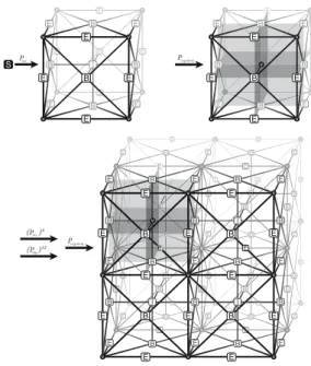
2.1. Hypergraph grammar model for genera-tion and adaptagenera-tion of three-dimensional mesh with point singularities. The process of generation of the three-dimensional computational mesh with hexahedral

elements starts with execution of the Pinit production,

presented in Fig. 1. It generates a hypergraph representing a single three-dimensional finite element. In the case of uniform mesh adaptations, we can prepare a sequence of graph grammar productions replacing the single element by a uniform cluster of elements. The model production Pinit break presented in Fig. 2 generates a uniform mesh

of eight elements. In order to get non-uniform mesh

refinements, we need to enforce the afore-mentioned 1-irregularity rule by breaking element interiors first, as is

expressed by productionPbreak intpresented in Fig. 3. An

example execution of the production over the eight finite element mesh is presented in Fig. 4. In the case of faces,

Fig. 1. Initial productionPinitthat generates a single cubic

ele-ment.

Fig. 2. Production breaking a single element into eight ele-ments.

a face can be broken only if two adjacent interiors have already been broken, or one adjacent interior has been broken and the face is located on the boundary of the

mesh. The case is illustrated with productionPbreak face

presented in Fig. 5. Finally, edges can be broken only if all adjacent faces have already been broken, or the edge is located on the boundary (and in such a scenario we need to check fewer adjacent faces). This is illustrated in Fig. 6

by productionPbreak edge.

2.2. Multi-frontal solver algorithm prescribed by hy-pergraph grammars. In order to apply the concept to a frontal solver algorithms, a simple 2D two finite element

example will be used. The domainΩis described by two

elements and fifteen nodes—two interiors, seven edges and six vertices (cf. Fig. 7). In the 2D FEM we utilize basis functions related to element nodes. In this example, as presented in Fig. 8, we have linear basis functions

(4)

572

Fig. 3. Production breaking an interior of a single element.

Fig. 4. Eight-element mesh after breaking the interior of the front element.

Fig. 5. ProductionPfacethat breaks a face.

Fig. 6. ProductionPedgethat breaks an edge.

1 2 3 4 5

6 7 8

11 12 13 14 15

Fig. 7. Sample computational domain for the frontal solver.

related to element vertices, i.e., to nodes 1, 3, 5, 11, 13 and 15, quadratic basis functions related to element edges, namely to nodes 2, 4, 6, 8, 10, 12 and 14, as well as quadratic basis functions related to element interiors,

namely to nodes 7 and 9. We construct the matrix

by integrating multiplications of these basis functions or their derivatives over a domain. Thus, matrix rows and columns correspond to basis functions and matrix entries correspond to multiplications of pairs of basis functions. Interior basis functions have support over a given element only, edge basis functions have support spread over one or two elements, vertex basis functions also have support spread over one or many elements.

The frontal solver introduced by Irons (1970) browses finite elements in a user-determined, arbitrary order. Due to its nature, it is sequential. Nodes (degrees of freedom) are aggregated into so-called frontal matrices.

Instead of generating just one large FEM matrix, it generates small matrices, called element frontal matrices. These matrices are obtained by integrating basis functions

1 2 3 4 5 6 7 8 9 10 11 12 13 14 15 1 2 3 4 5 6 7 8 9 10 11 12 13 14 15 88 3 0 1 2 10 5 4 1 2 3 4 5 6 7 8 9 10 11 12 13 14 15 9 3 4

Fig. 8. Example basis functions spread over element nodes: the basis function associated with vertex node 1 (black), ver-tex node 3 (dark gray) and verver-tex node 5 (light gray) (a), the basis function associated with edge node 6 (black), edge node 8 (dark gray) and edge node 10 (light gray) (b), the basis function associated with interior node 7 (black) and interior node 9 (dark gray) (c) .

(5)

Fig. 9. Processing of the right element by the frontal solver.

1 2 3 4 5

6

11 12 13 14 15

Fig. 10. Processing of the left element by the frontal solver.

over a given element. Thus, some entries in the element frontal matrix are fully assembled, and some are not. The row of the frontal matrix is called fully assembled, if all of its entries (integrals of products of pairs of basis functions) have been fully computed. This happens if both basis functions have support over a given element only, or the first of the basis functions has support over a given element only (since even the second basis functions also has support over some other element, its product with the first basis function is also zero). The fully assembled rows are self-contained and can be eliminated by the solver algorithm at any time. If a basis function has support defined only over a single element, we say that the node is reduced to the element only, and it has all its contributions already present in the element frontal matrix.

The aim of the frontal solver is to keep the frontal matrix as small as possible. To this end, it analyses the connectivity of the nodes and performs partial forward elimination of the fully assembled nodes. Fully assembled nodes have all of their contributions already present in the matrix, so no additional knowledge is necessary

to eliminate corresponding rows. Its mechanisms are

presented using an example of a two-element mesh. Since the order is arbitrary, we decided to add the nodes of the right element to the matrix first. Nodes 4, 5, 9, 10, 14 and 15 are proprietary to the right element and thus, we can call them fully assembled. Nodes 3, 8 and 13 are shared with the left element, and hence, will not be fully assembled until the frontal matrix associated with the left element is not merged with the frontal matrix associated with the right element.

The frontal solver browses elements one by one. It starts with generating a frontal matrix for the right element, for all the nodes (4, 5, 9, 10, 14, 15, 3, 8, 13). We put the fully assembled nodes (4, 5, 9, 10, 14, 15) in the upper part of the matrix. We perform partial forward elimination, eliminating all fully assembled nodes (4, 5,

9, 10, 14, 15). This is shown in Fig. 9. The upper triangular part of the frontal matrix has to be stored for future backward substitution. What is left is the reduced frontal matrix associated with nodes (3, 8, 13), which are not yet fully assembled. Such a reduced matrix is called the Schur complement matrix. The solver now moves to the left element (Fig. 10) and generates its frontal matrix (3, 8, 13, 1, 2, 6, 7, 11, 12), which is followed by adding the contribution that remained after processing the right element. This is illustrated in Fig. 11. Now, all nodes are fully assembled in a single matrix, so it is possible to perform full forward elimination.

The process is followed by backward substitution,

browsing elements in reverse order. The solver takes

advantage of the upper triangular form of the frontal matrix and computes the solution at each node, one by one. Such an approach allows us to keep the size of the matrix as small as possible by eliminating unknowns as soon as possible. Unfortunately, as mentioned before, in this case only the matrix operations can be parallelized due to the nature of the algorithm.

The multi-frontal solver introduced by Duff and Reid (1983; 1984) is the state-of-the-art direct solver algorithm for solving systems of linear equations, which is a generalization of the frontal solver algorithm (Irons, 1970). However, in the case of a multi-frontal solver, connectivity analysis is performed using a so-called elimination tree. A computational domain is decomposed into hierarchical subdomains, which account for the

elimination tree (Fig. 12). The construction of the

elimination tree for an arbitrary mesh is a complex task per se. It is done by constructing the graph representing the connectivities in the mesh, which is followed by

3 8 13 1 2 6 7 11 12 3 8 13 1 2 6 7 11 12 3 8 13 3 8 13 3 8 13 1 2 6 7 11 12 3 8 13 1 2 6 7 11 12 3 8 13 1 2 6 7 11 12 3 8 13 1 2 6 7 11 12

Fig. 11. Upper triangular form of the frontal matrix after pro-cessing the second element.

1 2 3 3 4 5 6 7 8 8 9 10 11 12 13 13 14 15 8 8 3 3 13 13

(6)

574

running graph partitioning algorithms such as nested dis-sections from METIS library (Karypis and Kumar, 2009). Usually, commercial solvers like the MUMPS (Duff and Reid, 1983; 1984) solver are not aware of the structure of the mesh, and they need to reconstruct the connectivity pattern by analysing the sparsity pattern of the matrix submitted to the solver. Note that such a matrix is already in its the global form, after the assembly of all element

frontal matrices. Another method for construction of

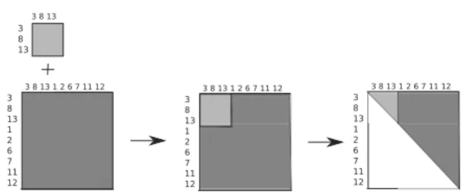
elimination trees is presented by Aboueisha et al. (2017). In the multi-frontal approach, the solver generates a frontal matrix for each element of the mesh. This is illustrated in Figs. 13 and 14. It eliminates fully assembled nodes within each frontal matrix, and merges the resulting Schur complement matrices at the parent level of the tree. This is illustrated in Fig. 15. The key difference with respect to the frontal matrix is that at the parent level the

solver works with a smaller matrix, which is a3×3matrix

obtained from the two Schur complements computed at its son nodes. In other words, the frontal matrix assembles element frontal matrices to a single frontal matrix and eliminates what is possible from the single matrix, while the multi-frontal solver utilizes multiple frontal matrices and thus allows us to reduce the size of the matrices at the parent nodes of the tree.

The first graph grammar productions are responsible for generation of the frontal element matrices. This is

done by productionsPagreg int responsible for generation

of the matrix entries associated with interior nodes, Pagreg boundary and Pagreg face responsible for generation

of matrix entries associated with boundary and interior

faces,Pagreg edgeandPagreg vertexresponsible for generation

of matrix entries associated with element edges and vertices. These graph grammar productions are illustrated in Fig. 16.

Having assembled the frontal matrix, it is now

1 2 6 7 11 12 3 8 13 1 2 6 7 11 12 3 8 13 1 2 6 7 11 12 3 8 13 1 2 6 7 11 12 3 8 13

Fig. 13. Partial forward elimination on the left element.

Fig. 14. Partial forward elimination on the right element.

1 2 6 7 11 12 3 8 13 1 2 6 7 11 12 3 8 13 1 2 6 7 11 12 3 8 13 1 2 6 7 11 12 3 8 13 4 5 9 10 14 15 3 8 13 4 5 9 10 14 15 3 8 13 4 5 9 10 14 15 3 8 13 4 5 9 10 14 15 3 8 13 3 8 13 3 8 13 3 8 13 3 8 13

Fig. 15. Full forward elimination of the interface problem ma-trix.

Fig. 16. Productions for assembly of an element frontal matrix.

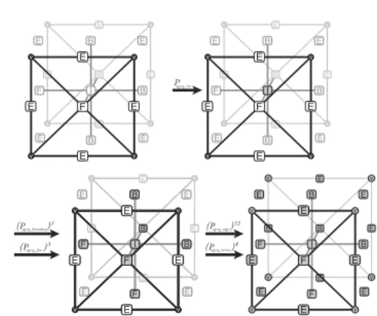
possible to start elimination of the fully assembled nodes. We can eliminate the interior node, which is denoted

by productionPelim int presented in Fig. 17, we can also

eliminate boundary faces, which is denoted by production Pelim faceas well as boundary edges and vertices, compare

productionsPelim edgeandPelim vertexin Fig. 17.

Having adjacent elements with frontal matrices and eliminated interior and boundary nodes, we can now merge the frontal matrices into one matrix and eliminate

fully assembled nodes from the common face. It

is expressed by productionsPmerge eliminate illustrated in

Fig. 18. This procedure of merging frontal matrices and eliminating fully assembled nodes located on common faces is repeated until all the nodes in the mesh are eliminated.

3. Linear computational cost solver for

three-dimensional meshes with point

singularities

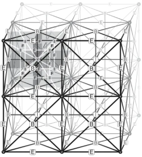
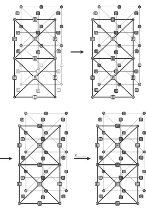
In the case of a mesh with point singularities, as the one presented in Fig. 19, we can take advantage of the multi-level structure of the computational grid in the following way: We start with the grid presented in the

right panel in Fig. 2. The first step is to execute the

multi-frontal solver algorithm for all elements, except the elements located closest to the point singularity.

(7)

Fig. 17. Squashed productions Pelim int, Pelim boundary, Pelim edge

andPelim vertex that execute elimination of the interior,

boundary nodes, edges and an internal vertex.

Fig. 18. ProductionPmerge eliminate for merging two frontal

ma-trices and elimination of fully assembled nodes from a common face.

Fig. 19. Three-dimensional mesh with a single point singularity.

elements on the top level we execute the following

chain of productions: Pagreg init → Pagreg boundary →

Pagreg face → Pagreg edge → Pagreg vertex. The

next step is to eliminate entries that resulted from the previously aggregated element contributions, which can be achieved by executing the following chain

of productions: Pelim boundary → Pelim edge →

Pelim vertex.

Finally, we merge the frontal matrices, by executing

productionsPmerge eliminateas many times as necessary to

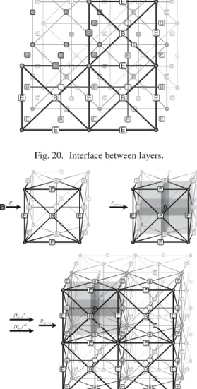
end up with the interface of the top level with respect to the next level, as presented in Fig. 20. We store the Schur complement matrix associated with the interface.

At this point, we can aggregate the frontal

matrix associated with the element nearest to the point

singularity, by executing productions Pagreg init →

Pagreg boundary → Pagreg face → Pagreg edge →

Pagreg vertex.

As the next step, we can merge the element frontal matrix with the Schur complement matrix, by executing

production Pmerge with Schur. This results in a fully

assembled matrix and we can solve the problem close to the singularity.

If a more accurate solution is desirable, we can break the element neighboring the singularity by executing the

productionPbreak singularitypresented in Fig. 21, preserving

the Schur complement adjacent to the broken element. At this point, we continue solving the problem over the newly refined elements by executing the following

chain of productions: Pagreg init → Pagreg boundary →

Pagreg face → Pagreg edge → Pagreg vertexthat generate

the element frontal matrices, followed by productions Pelim boundary → Pelim edge → Pelim vertex, together

with Pmerge with Schur reutilizing the Schur complement

matrix for the interface with the other part of the mesh.

4. Computational complexity of a

sequential hypergraph grammar-based

solver for three-dimensional meshes with

point singularities

As a diligent estimation of the exact computational cost for the three-dimensional version of the solver would be a very strenuous task, we limit ourselves to a rough approximation of the computational complexity, ignoring

the constants. Note thatpis assumed to be constant over

the entire domain. In fact, due to numerical unstability,

p very rarely exceeds 10 and hence this assumption is

fair. In case of the hp version of the FEM algorithm,

where both h and p are variable, we can assume that

p = pmax = constto approximate the upper boundary

of the cost.

Lemma 1. The computational complexity of the

(8)

576

Fig. 20. Interface between layers.

Fig. 21. Hypergraph grammar derivation of a grid with a point singularity.

freedomN and the polynomial order of approximationp

for the three-dimensional grid with a point singularity is

equal toT(p, N) =O(Np6).

Proof. A three-dimensional element hasO(p)degrees of

freedom over an element edge,O(p2)degrees of freedom

over an element face and O(p3) degrees of freedom

over an element interior. The number of base functions spanned over the element vertices is constant and hence

independent of p. The computational complexity of the

elimination of the interior-related degrees of freedom is

of the order of O((p+p2 +p3)2p3) = O(p9). The

computational complexity of the static condensation is of

the order of O(Nep9), whereNe denotes the number of

elements.

The remaining degrees of freedom over the faces and

edges are eliminated level by level (layer by layer), and the computational complexity of elimination of a single level

is of the order ofO((p2 +p)3) = O(p6). The number

of elementsNe is of the order of O(Ne) = O(N/p3),

and the number of levels k is of the order of O(k) =

O(N/p3_{). Thus the total computational complexity is}

of the order ofO(Nep9+kp6) = O(Np6 +Np3) =

O(Np6_{), which completes the proof.}

The proven complexity depends onpthat in theory

is variable. However, as mentioned above, in practice

it very rarely exceeds 10 due to severe numerical

problems caused by high order polynomials. For the

case ofhp-refinements, where the polynomial orders of

approximations vary, we can use the above estimate as the upper bound for the computational cost, assuming the uniform distribution of the maximum utilized polynomial order of approximation.

5. Memory usage of a hypergraph

grammar-based solver for

three-dimensional meshes with point

singularities

Memory usage in case of the hypergraph grammar driven solver for three-dimensional meshes with point singularities remains linear with respect to the number of

the degrees of freedomN. The order of memory usage is

roughly estimated in the lemma below.

Lemma 2. Memory usageMof the solver with respect to

the number of degrees of freedomNand polynomial order

of approximationpfor the three-dimensional grid with a

point singularity is of the order ofM(N, p) =O(Np3).

Proof. A three-dimensional element contains O(p)

degrees of freedom over element edges,O(p2)degrees of

freedom over element faces andO(p3)degrees of freedom

over element interiors. The memory usage complexity of storing an element frontal matrix is of the order of

O((p+p2₊_p3₎2_{) =} _O₍_p6_{). The total memory usage}

complexity of storing element frontal matrices is of the

order ofO(Nep6). The matrices at higher levels contain

contributions from faces and edges and the memory usage complexity of storing such a matrix is of the order of

O((p2 ₊_p₎2_{) =} _O₍_p4_{). The number of elements} _N

e

is of the order ofO(Ne) = O(N/p3), and the number

of levelsk is of the order ofO(k) = O(N/p3). Thus

the total memory usage complexity is of the order of

(9)

6. Theoretical estimates of computational

complexity for parallel shared memory

machine solver execution

In this section we roughly estimate a theoretical computational complexity of the fastest version of the solvers presented in this paper which is the parallel hypergraph grammar solver for three-dimensional meshes with point singularities.

We assume that execution takes place on a shared

memory machine. For a message passing parallelism

model, the cost of communication needs to be included. Another important assumption is the infinite number of cores, so that the scalability is unrestricted. While it is an idealized scenario, in reality it would be enough to find a right balance between the problem size and the amount of cores available to optimize the performance. In the worst case of severe misconfiguration, the complexity of this algorithm will be reduced to linear. A good analogy would be a comparison to a binary search tree which on the average offers logarithmic time for all basic operations, but in its extreme, imbalanced version, the complexity deteriorates to linear.

Lemma 3. The computational complexity of the parallel

solver with respect to the number of degrees of freedom

Nand polynomial order of approximationpfor the

three-dimensional grid with a point singularity is of the order of

O(p6_log(_N/p3_)).

Proof. A three-dimensional element (see Fig. 1) contains

O(p) degrees of freedom over element edges, O(p2)

degrees of freedom over element faces andO(p3)degrees

of freedom over element interiors. The number of the degrees of freedom over vertices is obviously constant and

it does not depend onp.

The computational complexity of elimination of

in-terior degrees of freedom is of the order of O(p3(p+

p2 ₊ _p3₎2_{) =} _O₍_p9_{), since we eliminate} _p3 _interior

nodes from the element matrix with all element degrees

of freedom of order of p+p2+p3 (subtractp3 rows

from an element matrix). The degrees of freedom over the remaining faces and edges are eliminated level by level (layer by layer), and the computational complexity of their elimination over a single level is of the order

of O((p2 +p)3) = O(p6). This is because we have

the order ofp2+pdegrees of freedom on the interface

and the same order of degrees of freedom in the entire

layer. In parallel, we construct an elimination tree

withO(log(k))levels, wherekis the previously defined

number of the refinement levels. In particular, the number

of levels k is of the order of O(k) = O(N/p3) and

thus O(log(k)) = O(log(N/p3)). This is why the

computational complexity of the parallel solver isO(p9+

p6_log(_N/p3_{)) =} _O₍_p6_log(_N/p3_)). _{This is because}

we perform parallel elimination of elements interior,

followed by the elimination of the refinement levels on

particular layers of the tree with depth O(log(N/p3)).

This completes the proof.

7. Numerical results for a multi-thread

shared memory GALOIS solver

To conclude the considerations above, we present a series of numerical results illustrating the performance of the

described solver. We used the GALOIS environment

(Goik et al., 2014; Paszy´nska et al., 2015; Pingali et al., 2011) for solver implementation. We first illustrate the linear scalability of the sequential solver when executed on the sequence of grids refined towards point 19, edge 22, and face 23. The scalability of the sequential code is illustrated in Figs. 24–27 for the point singularity, in Figs. 28–31 for the edge singularity, and in Figs. 32–35 for the face singularity.

The mesh with a point singularity yields linear computational cost, which can be read from Figs. 24–27, for the grids with uniform polynomial order of

approximationsp = 2,3,4,5.The linear computational

cost of the sequential solver is also obtained for the mesh with an edge singularity, which can be read from Figs. 28–31, for the polynomial orders of approximations

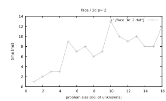
p = 2,3,4,5. Finally, the mesh with face singularity

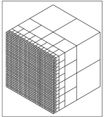
Fig. 22. Mesh refined towards an edge.

(10)

578

also delivers a linear cost, for different polynomial orders,

which can be read from Figs. 32–35. For very small

grids, and for quadratic basis functions, the computational problem is very small, and there are some oscillations in the time measurements.

From these plots we can observe, that if the problem size becomes large enough, we recover linear computational cost not only for the point singularity, but also for the edge and the face.

Second, we illustrate the scalability of the parallel solver when executed on the fixed mesh refined towards points 36–39, edges 40–43, and faces 44–47. The experiments were performed on a GILBERT shared-memory Linux cluster node using up to 16 cores.

We can observe the logarithmic decrease in the computation time for the grid with a point singularity, when increasing the number of cores, as presented in Figs. 36–39, for different polynomial orders of approximation. A similar logarithmic decrease can be observed for the grids with edge singularities, as presented in Figs. 40–43, and for the grids with face singularities, as presented in Figs. 44–47.

We would like to point out that horizontal lines in Figs. 24–35 presenting the sequential results contain the problem size, while the horizontal lines in Figs. 36–47 presenting the parallel results contain the number of

utilized cores. Each parallel experiment has been

executed on a single mesh with fixed size. The

size of the mesh can be obtained by looking at the sequential computations, where the sequential execution time matches the parallel execution time with a single core. Notice that the theoretical result concerning the logarithmic computational cost of the parallel algorithm assumes an infinite number of cores, and we are restricted here to the case of 16 cores only, so producing an ideal logarithmic estimate is rather impossible in practice. From these plots we can observe that if the problem size becomes large enough (if we increase the polynomial order over the mesh nodes), the parallel code scales very well. For low computational cost grids (low polynomial order over the mesh nodes) the tasks are not heavy and the scheduling is more expensive than execution.

8. Conclusions

The main and most significant achievement of this work is creation of models applicable to a wide class of adaptive algorithms. The formal methodology used to achieve this goal was the hypergraph grammar formalism. All the graph grammar productions presented in this work can also be applied to three-dimensional grids with arbitrary

refinements. However, for the sake of simplicity, we

restricted ourselves here to the subset of hypergraph grammar productions expressing the grids with single point singularities. Nevertheless, in the numerical sections

0 2 4 6 8 10 12 0 500 1000 1500 2000 2500 3000 time [ms]

problem size [no. of unknowns] point / 3d p= 2

("./point_3d_2.dat")

Fig. 24. Scalability of sequential hypergraph grammar-based execution over the sequence of meshes refined toward

the point singularity, with uniformp= 2.

0 20 40 60 80 100 120 140 160 0 1000 2000 3000 4000 5000 6000 7000 8000 time [ms]

0 200 400 600 800 1000 1200 1400 2000 4000 6000 8000 10000 12000 14000 16000 18000 time [ms]

0 1000 2000 3000 4000 5000 6000 7000 8000 9000 0 5000 10000 15000 20000 25000 30000 35000 time [ms]

(11)

1 1.5 2 2.5 3 3.5 4 200 400 600 800 1000 1200 1400 1600 1800 time [ms]

problem size [no. of unknowns] edge / 3d p= 2

("./edge_3d_2.dat")

the edge singularity, with uniformp= 2.

0 5 10 15 20 25 30 35 40 500 1000 1500 2000 2500 3000 3500 4000 4500 5000 time [ms]

("./edge_3d_3.dat")

0 50 100 150 200 250 300 350 1000 2000 3000 4000 5000 6000 7000 8000 9000 10000 11000 time [ms]

("./edge_3d_4.dat")

1 . 11 511 211 311 4111 4. 11 4511 4211 4311 . 111 5111 2111 3111 41111 4. 111 45111 42111 43111 . 1111 06 8t i 8 me

[ s] prt 8 m6ot ib] l ] z nbf b] u bme t kwt d gk [ / =

("ldt kwt _gk_=lka0")

0 0.5 1 1.5 2 0 100 200 300 400 500 600 700 800 time [ms]

problem size [no. of unknowns] face / 3d p= 2

("./face_3d_2.dat")

the face singularity, with uniformp= 2.

0 1 2 3 4 5 6 200 400 600 800 1000 1200 1400 1600 1800 2000 2200 time [ms]

("./face_3d_3.dat")

0 5 10 15 20 25 30 35 0 500 1000 1500 2000 2500 3000 3500 4000 4500 time [ms]

("./face_3d_4.dat")

0 . 0 50 10 20 300 3. 0 350 310 0 3000 . 000 4000 5000 6000 1000 7000 2000 8t i m ei [s

] pr obmi [ tl m ezr n r f uzkzr wz[ s facm / 4d ] = 6

("n/facm_4d_6nda8")

(12)

580 0 2 4 68 61 60 62 64 8 1 0 2 4 68 61 60 62 time [ms]

Fig. 36. Scalability of parallel hypergraph grammar-based exe-cution over the mesh refined toward the point

singular-ity, with uniformp= 2.

01 21 31 41 51 61 71 81 911 991 901 1 0 3 5 7 91 90 93 95 time [ms]

011 211 311 411 511 611 711 811 911 0111 0011 1 2 4 6 8 01 02 04 06 time [ms]

0 2000 4000 6000 8000 1000 3000 5000 0 4 8 3 7 20 24 28 23 time [ms]

2 4 6 8 10 12 14 16 18 20 0 2 4 6 8 10 12 14 16 time [ms]

("./edge_3d_2.dat")

Fig. 40. Scalability of parallel hypergraph grammar-based exe-cution over the mesh refined toward the edge

24 26 28 21 20 64 66 68 61 60 t 4 4 6 8 1 0 24 26 28 21 im e[ s e ]p r obl z[ e ] mn[ s. bf bu k. w. bd . ] p [ g/ [ 3 t g r = t ("f3[ g/ [ _t g_t fgai")

1 . 1 511 5. 1 211 2. 1 311 1 2 4 0 6 51 52 54 50 8t i m ei [s

] pr obmi [ tl m ezr n r f uzkzr wz[ s mdgm / 3d ] = 4

("n/mdgm_3d_4nda8")

1 . 11 511 211 311 4111 4. 11 4511 4211 1 . 5 2 3 41 4. 45 42 06 8t i 8 me

[ s] prt 8 m6ot ib] l ] z nbf b] u bme t kwt d gk [ / =

("ldt kwt _gk_=lka0")

(13)

0 2 4 6 8 10 12 14 0 2 4 6 8 10 12 14 16 time [ms]

("./face_3d_2.dat")

Fig. 44. Scalability of parallel hypergraph grammar-based exe-cution over the mesh refined toward the face

0 2 4 6 81 80 82 84 1 0 2 4 6 81 80 82 84 time [ms]

("./face_3d_3.dat")

02 04 06 08 01 42 44 46 48 41 2 4 6 8 1 02 04 06 08 time [ms]

("./face_3d_6.dat")

20 30 40 50 60 70 80 90 100 110 120 0 2 4 6 8 10 12 14 16 time [ms]

("./face_3d_5.dat")

we analyzed three-dimensional meshes refined towards

a point, an edge and a face. We proved theoretically

and experimentally the linear computational cost of the algorithm. We also showed the theoretical logarithmic computational cost of the parallel execution, especially

for polynomial orders of approximationp > 2, and we

have verified the parallel scalability on a shared-memory

Linux cluster node with 16 cores. The scalability of

the hypergraph-grammar-based solvers does not depend on the PDE being solved, but rather on the structure

of the computational mesh generated by the h adaptive

procedure.

Acknowledgment

The work presented in this paper is supported

by the Polish National Science Center (grant no. DEC-2015/17/B/ST6/01867).

References

Aboueisha, H., Calo, V.M., Jopek, K., Moshkov, M., Paszy´nska, A., Paszy´nski, M. and Skotniczny, M. (2017). Element

partition trees for h-refined meshes to optimize direct

solver performance. Part I: Dynamic programming, Inter-national Journal of Applied Mathematics and Computer Science 27(2): 351–365, DOI: 10.1515/amcs-2017-0025.

Bao, G., Hu, G. and Liu, D. (2012). Anh-adaptive finite element

solver for the calculations of the electronic structures, Jour-nal of ComputatioJour-nal Physics 231(14): 4967–4979.

Belytschko, T. and Tabbar, M. (1993). h-adaptive finite

element methods for dynamic problems, with emphasis on localization, International Journal for Numerical Methods in Engineering 36(24): 4245–4625.

Duff, I.S. and Reid, J.K. (1983). The multifrontal solution of indefinite sparse symmetric linear, ACM Transactions on Mathematical Software 9(3): 302–325.

Duff, I.S. and Reid, J.K. (1984). The multifrontal solution of unsymmetric sets of linear equations, SIAM Journal on Sci-entific and Statistical Computing 5(3): 633–641.

Flasi´nski, M. and Schaefer, R. (1996). Quasi context sensitive graph grammars as a formal model of FE mesh generation, Computer-Assisted Mechanics and Engineering Science 3: 191–203.

Goik, D., Paszy´nski, M., Lenharth, A., Nguyen, D. and

Pingali, K. (2014). Graph grammar based multi-thread

multi-frontal direct solver with Galois scheduler, Procedia Computer Science 29: 960–969.

Grabska, E. (1993a). Theoretical concepts of graphical

modeling. Part I: Realization of CP-graphs, Machine Graphics and Vision 1(2): 3–38.

Grabska, E. (1993b). Theoretical concepts of graphical

modeling. Part II: CP-graph grammars and languages, Ma-chine Graphics and Vision 2(2): 149–178.

(14)

582

Habel, A. and Kreowski, H.J. (1987a). May we introduce to you: Hyperedge replacement, in H. Ehrig et al. (Eds.), Graph-Grammars and Their Application to Computer Science, Lecture Notes in Computer Science, Vol. 291, Springer, Berlin/Heidelberg, pp. 5–26.

Habel, A. and Kreowski, H.J. (1987b). Some structural

aspects of hypergraph languages generated by hyperedge replacement, in F.J. Brandenburg et al. (Eds.), STACS 87, Lecture Notes in Computer Science, Vol. 247, Springer, Berlin/Heidelberg, pp. 207–219.

Irons, B.M. (1970). A frontal solution program for finite-element analysis, International Journal for Numerical Methods in Engineering 2: 5–32.

Karypis, G. and Kumar, V. (2009). MeTis: Unstructured Graph Partitioning and Sparse Matrix Ordering System, Version 4.0,http://www.cs.umn.edu/˜metis.

Paszy´nska, A., Grabska, E. and Paszy´nski, M. (2012a). A

graph grammar model of thehpadaptive three dimensional

finite element method, Part I, Fundamenta Informaticae 114(2): 149–182.

Paszy´nska, A., Grabska, E. and Paszy´nski, M. (2012b). A graph grammar model of the HP adaptive three dimensional finite element method, Part II, Fundamenta Informaticae 114(2): 183–201.

Paszy´nska, A., Paszy´nski, M. and Grabska, E. (2009). Graph

transformations for modeling hp-adaptive finite element

method with mixed triangular and rectangular elements, in G. Allen et al. (Eds.), ICCS 2009, Lecture Notes in Computer Science, Vol. 5545, Springer, Berlin/Heidelberg, pp. 875–884.

Paszy´nska, A., Paszy´nski, M., Jopek, K., Wo´zniak, M., Goik, D., Gurgul, P., AbouEisha, H., Moshkov, M., Calo, V.M., Lenharth, A., Nguyen, D. and Pingali, K. (2015). Quasi-optimal elimination trees for 2D grids with singularities, Scientific Programming 2015, Article ID: 303024, DOI:10.1155/2015/303024.

Paszy´nski, M. (2009). On the parallelization of self-adaptive

hp-finite element methods, Part I: Composite

programmable graph grammar model, Fundamenta

Informaticae 4(93): 411–434.

Paszy´nski, M. (2016). Fast Solvers for Mesh-Based Computa-tions, CRC Press, Boca Raton, FL.

Paszy´nski, M. and Paszy´nska, A. (2008). Graph transformations

for modeling parallelhp-adaptive finite element method,

in R. Wyrzykowski et al. (Eds.), PPAM 2007, Lecture

Notes in Computer Science, Vol. 4967, Springer,

Berlin/Heidelberg, pp. 1313–1322.

Paszy´nski, M. and Schaefer, R. (2010). Graph grammar-driven parallel partial differential equation solver, Concurrency and Computation Practice and Experience 22: 1063–1097. Pingali, K., Nguyen, D., Kulkarni, K., Burtscher, K.M., Hassaan, M.A., Kaleem, R., Lee, T.-H., Lenharth, A., Manevich, R., Mendez-Lojo, M., Prountzos, D. and Sui, X. (2011). The Tao of parallelism in algorithms, 32nd ACM SIGPLAN Conference on Programming Language Design and Implementation, San Jose, CA, USA, pp. 12–22.

Ryszka, I., Paszy´nska, A., Grabska, E., Sieniek, M. and Paszy´nski, M. (2015a). Graph transformation systems for modeling three dimensional finite element method, Part I, Fundamenta Informaticae 140(2): 129–172.

Ryszka, I., Paszy´nska, A., Grabska, E., Sieniek, M. and Paszy´nski, M. (2015b). Graph transformation systems for modeling three dimensional finite element method, Part II, Fundamenta Informaticae 140(2): 173–203.

´Slusarczyk, G. and Paszy´nska, A. (2013). Hypergraph grammars

inhp-adaptive finite element method, Procedia Computer

Science 18: 1545–1554.

Piotr Gurgul was born in 1987. He gradu-ated from a combined MSc and BEng program in computer science at the AGH University of Science and Technology in Krak´ow in 2011, and from a BBA program in management from the Krak´ow University of Economics in 2012. In 2014 he obtained his PhD in computer science at the AGH University of Science and Technology. His scientific interests focus on the hp-adaptive finite element method and adaptive solvers. Cur-rently he works at Dropbox Inc. in California.

Konrad Jopek is a PhD student at the

Depart-ment of Computer Science of the AGH Univer-sity of Science and Technology. He is a co-author of several publications about fast solvers for the finite element method. His research interests fo-cus on numerical methods, parallel algorithms, highly-scalable software and low-level progam-ming. His PhD advisors are Maciej Paszy´nski and Anna Paszy´nska.

Keshav Pingali is a W.A.“Tex” Moncrief Chair

of Grid and Distributed Computing, a profes-sor at the Department of Computer Science and the Institute for Computational Engineering and Sciences, University of Texas, Austin. His current research interests include methodologies and tools for programming multicore processors, with a focus on irregular applications from do-mains like graphics, social networks, and data mining.

Anna Paszy ´nska received her PhD (2007) in computer science from the Institute of Fun-damental Technological Research of the Pol-ish Academy of Sciences in Warsaw, Poland. She currently works as an assistant professor at the Faculty of Physics, Astronomy and Ap-plied Computer Science, Jagiellonian University in Krak´ow, Poland. Her research interests in-clude evolutionary algorithms, graph grammar and computer aided design.

Received: 13 June 2017 Revised: 24 January 2018 Re-revised: 10 March 2018 Accepted: 19 April 2018