Identification of Nonlinear Systems Using Radial Basis Function Neural Network
Original Citation
Pislaru, Crinela and Shebani, Amer (2014) Identification of Nonlinear Systems Using Radial Basis
Function Neural Network. International Journal of Computer, Information, Systems and Control
Engineering , 8 (9). pp. 1528-1533.
This version is available at http://eprints.hud.ac.uk/23885/
The University Repository is a digital collection of the research output of the
University, available on Open Access. Copyright and Moral Rights for the items
on this site are retained by the individual author and/or other copyright owners.
Users may access full items free of charge; copies of full text items generally
can be reproduced, displayed or performed and given to third parties in any
format or medium for personal research or study, educational or not-for-profit
purposes without prior permission or charge, provided:
•
The authors, title and full bibliographic details is credited in any copy;
•
A hyperlink and/or URL is included for the original metadata page; and
•
The content is not changed in any way.
For more information, including our policy and submission procedure, please
contact the Repository Team at: [email protected].
Abstract—This paper uses the radial basis function neural
network (RBFNN) for system identification of nonlinear systems. Five nonlinear systems are used to examine the activity of RBFNN in system modeling of nonlinear systems; the five nonlinear systems are dual tank system, single tank system, DC motor system, and two academic models. The feed forward method is considered in this work for modelling the non-linear dynamic models, where the K-Means clustering algorithm used in this paper to select the centers of radial basis function network, because it is reliable, offers fast convergence and can handle large data sets. The least mean square method is used to adjust the weights to the output layer, and Euclidean distance method used to measure the width of the Gaussian function.
Keywords—System identification, Nonlinear system, Neural
networks, RBF neural network.
I. INTRODUCTION
HE concept of a neural network was originally conceived as an attempt to model the biophysiology of the brain. An artificial neural network (ANN) offers a potential solution for problems which require complex data analysis and promise to form the future basis of an improved alternative to current engineering practice. The neural networks have many applications in various fields of study, including modeling and control of linear and nonlinear systems. Neural networks have been developed in different ways, where various algorithms and methods have been applied, such as backpropagation (BP) rule and radial basis function (RBF) [1]–[3]. Artificial neural networks (ANNs) are often used for applications where it is difficult to state explicit rules. Often it seems easier to describe a problem and its solution by giving examples; if sufficient data is available a neural network can be trained. There is a wide range of application domains where ANNs are being used, including classification, compression, noise reduction, optimization, prediction, and recognition. Neural networks with their remarkable ability to derive meaning from complicated or imprecise data can be used to extract patterns and detect trends that are too complex to be noticed by either humans or other computer techniques. A trained neural network can be thought of as an "expert" in the category of information it has been given to analyze. This expert can then be used to provide projections given new situations of interest. Identification of nonlinear systems based on RBFNN was done by many researchers but without mention about the main three parameters in RBFNN, and how they selected these
C. P. and A. S. are with the Institute of Railway Research, UK (e-mail:
parameters (centers, width and weights). Other researchers used the genetic algorithm to improve the RBFNN performance; this will be a more complicated identification process [4]–[15].
II.ARTIFICIAL NEURAL NETWORKS (ANNS)
A.Simple Perceptron
The simple perceptron shown in Fig. 1, it is a single processing unit with an input vector X = (x0,x1, x2…xn). This
vector has n elements and so is called n-dimensional vector. Each element has its own weights usually represented by the n-dimensional weight vector, e.g. W = (w0,w1,w2...wn).
Fig. 1 Simple perceptron diagram
The output y can be described by the following equation: ∑ (1) where are the weights and are the inputs [2], [16]–[19].
B.Multilayer Perceptron
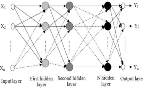
Multilayer perceptron, are constructed from multiple layers of elements, neurons or nodes, such as in Fig. 2, it consists of units that constitute the input layer, an output layer and a number of intermediate layers (hidden layers).
Fig. 2 Multilayer perceptrons diagram
The network requires a set of data as inputs to the input layer. The outputs of the input layer are then fed as weighted
Identification of Nonlinear Systems Using Radial
Basis Function Neural Network
C. Pislaru, A. Shebani
T
inputs to the first hidden layer. The outputs from the first hidden layer are fed as weighted inputs to the second hidden layer and so on. This process continues until the output layer is reached [1], [2], [13], [16], [19].
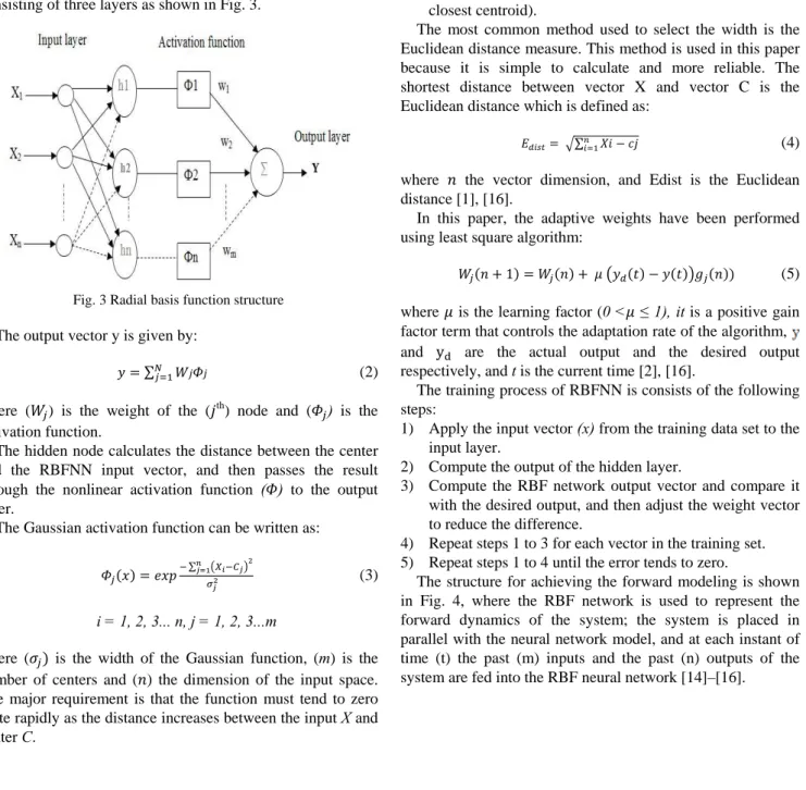
C.Radial Basis Function Neural Network (RBFNN)
Feed-forward layered neural networks have increasingly been used in many areas such as modeling and control of non-linear systems. One example of a feed forward neural network is the Radial Basis Function (RBF) network. The RBF network can be regarded as a special three layer network, including input, hidden and output layers. Full explanations of the connections of these layers together with the activation function are given in the next sections. The performance of the RBF depends on the proper selection of three important parameters (centers, widths and weights).
The RBF neural network has a feed forward structure consisting of three layers as shown in Fig. 3.
Fig. 3 Radial basis function structure The output vector y is given by:
∑ (2)
where ( ) is the weight of the ( th) node and ( ) is the activation function.
The hidden node calculates the distance between the center and the RBFNN input vector, and then passes the result through the nonlinear activation function ( ) to the output layer.
The Gaussian activation function can be written as: ∑
(3)
i = 1, 2, 3... n, j = 1, 2, 3...m
where ( is the width of the Gaussian function, (m) is the number of centers and ( ) the dimension of the input space. The major requirement is that the function must tend to zero quite rapidly as the distance increases between the input X and center C.
The Radial Basis Function Network consists of three important parameters, centers, width and weights. The values of these parameters are generally unknown and may be found during the learning process of the network. The major problem which therefore remains is one of how to select an appropriate set of RBF centers. To overcome this problem, the network requires some strategy for selecting the adequate set of centers, hence clustering algorithm have been used extensively [2], [13], [16], [19].
The K-Means clustering algorithm is used in this paper for selecting the centers, because of its simplicity and ability, to produce good results. The K means algorithm will do the following three steps until convergence such as in Fig. 5, iterate until stable (no object move group):
1) Determine the centroid coordinate
2) Determine the distance of each object to the centroids 3) Group the object based on minimum distance (find the
closest centroid).
The most common method used to select the width is the Euclidean distance measure. This method is used in this paper because it is simple to calculate and more reliable. The shortest distance between vector X and vector C is the Euclidean distance which is defined as:
∑ (4)
where the vector dimension, and Edist is the Euclidean distance [1], [16].
In this paper, the adaptive weights have been performed using least square algorithm:
(5)
where is the learning factor (0 < ≤ 1), it is a positive gain factor term that controls the adaptation rate of the algorithm, and y are the actual output and the desired output respectively, and t is the current time [2], [16].
The training process of RBFNN is consists of the following steps:
1) Apply the input vector (x) from the training data set to the input layer.
2) Compute the output of the hidden layer.
3) Compute the RBF network output vector and compare it with the desired output, and then adjust the weight vector to reduce the difference.
4) Repeat steps 1 to 3 for each vector in the training set. 5) Repeat steps 1 to 4 until the error tends to zero.
The structure for achieving the forward modeling is shown in Fig. 4, where the RBF network is used to represent the forward dynamics of the system; the system is placed in parallel with the neural network model, and at each instant of time (t) the past (m) inputs and the past (n) outputs of the system are fed into the RBF neural network [14]–[16].
Fig. 4 Series-parallel identification schemes
The system is governed by the following nonlinear difference equation:
, … . . , , , , … . , (6)
where: (.) is the plant output, and (.) is the input sequences. The neural based identification model is assumed to have the same structure as the plant and is given by: , … . . , , , , . , (7)
where . represents the non-linear input-output map of the network. Simulation Results Simulations have been performed using the RBF neural network. Various non-linear plants were tested and very good results were obtained. Five different plants were used as examples to show the properties of the radial basis function neural network (RBFNN). Fig. 5 is a block diagram of a series-parallel model which is used in this paper to system identification of nonlinear systems. The output of the plant and the network are compared and the resulting error is used to update the network parameters the weights. Fig. 5 Series-parallel identification schemes A.Dual Tank System The system in consideration consists of two interconnected water tanks linked together by an orifice. The water is fed into the system using an electrical water pump, the pump switched ON to move the water level in tank one to a certain level. As a result, the water level in tank two will rise with a certain rate until it reached a steady state level. The scheme of the system is given in Fig. 6. The inlet water quantity is denoted by qi, the outlet quantities are q1 and q2 respectively. The water levels are denoted by L1 and L2. The cross sections of a dual tank are A1 and A2. The cross sections of the tubes are denoted by R1 and R2. Fig. 6 Dual tank system The following differential equations describing the process dynamics of the dual tank [20]–[23]: (8)
(9)
(10)
(11) where: the system output to be L , it is the height of the fluid in the tank2; and the system input to be q , it isthe flow into the tank1.
The dual tank system response and RBFNN response are shown in Fig. 7.
Fig. 7 System output and RBFNN output
0 0.5 1 1.5 2 2.5 3 0 0.02 0.04 0.06 0.08 0.1 0.12 Time (seconds) A m pl it ude System response RBFNN response
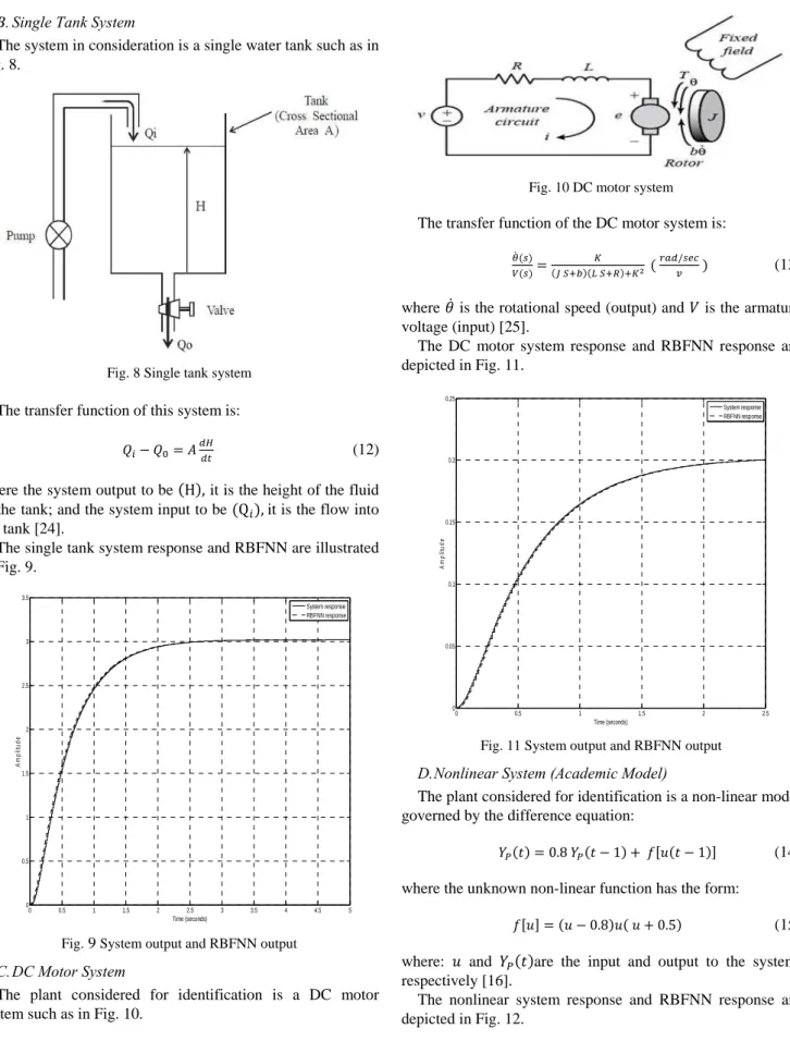
B.Single Tank System
The system in consideration is a single water tank such as in Fig. 8.
Fig. 8 Single tank system
The transfer function of this system is:
(12) where the system output to be H , it is the height of the fluid in the tank; and the system input to be Q , it is the flow into the tank [24].
The single tank system response and RBFNN are illustrated in Fig. 9.
Fig. 9 System output and RBFNN output
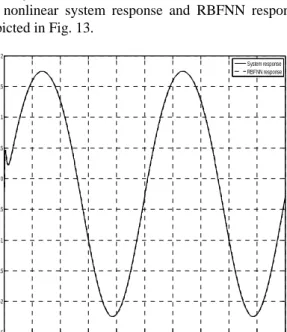
C.DC Motor System
The plant considered for identification is a DC motor system such as in Fig. 10.
Fig. 10 DC motor system The transfer function of the DC motor system is:
/ (13) where is the rotational speed (output) and is the armature voltage (input) [25].
The DC motor system response and RBFNN response are depicted in Fig. 11.
Fig. 11 System output and RBFNN output
D.Nonlinear System (Academic Model)
The plant considered for identification is a non-linear model governed by the difference equation:
. (14)
where the unknown non-linear function has the form:
. . (15) where: and are the input and output to the system, respectively [16].
The nonlinear system response and RBFNN response are depicted in Fig. 12. 0 0.5 1 1.5 2 2.5 3 3.5 4 4.5 5 0 0.5 1 1.5 2 2.5 3 3.5 Time (seconds) Amp li tu d e System response RBFNN response 0 0.5 1 1.5 2 2.5 0 0.05 0.1 0.15 0.2 0.25 Time (seconds) A m pl it ude System response RBFNN response
Fig. 12 System output and RBFNN output
E.Nonlinear System (Academic Model)
The plant considered for identification is a non-linear model governed by the equation:
. . . . (16)
where the unknown non-linear function has the form
. (17) The and are the input and output to the system, respectively [16], [21].
The nonlinear system response and RBFNN response for are depicted in Fig. 13.
Fig. 13 System output and RBFNN output III. CONCLUSION
Simulation results show that the RBF neural network exhibits good performance and ability in modelling dynamic systems. It also found that the response of the desired signal
was heavily dependent on the value of the learning factor, centers, width and weights of RBF. Also, the simulation results show that the radial basis function neural network is a powerful tool for nonlinear system modelling; it is an accurate method for modeling the nonlinear systems. One of the main advantages of RBFNN is that the ability of quick modifying in the modelling during the change of the dynamics of the process.
REFERENCES
[1] S. Haykin, “Neural Networks, A Comprehensive Foundation”, Prentice-Hall Inc., second edition, USA, 1999.
[2] Bose, and P. Liang, “Neural Network Fundamentals with Graphs, Algorithms and Applications”, McGraw-Hill series in Electrical and Computer Engineering, USA, 1996.
[3] Kriesel, “A Brief Introduction to Neural Networks”, Zeta2, University of Bonn, Germany, 2005.
[4] J. Li, and F. Zhao, “Identification of Dynamical Systems Using Radial Basis Function Neural Networks with Hybrid Learning Algorithm”, Systems and Control in Aerospace and Astronautics, ISSCAA 2006. [5] M. Y. Mashor, “Nonlinear system identification using RBF networks
with linear input connections”, Malaysian Journal of Computer Science, Vol. 11 No. 1, June 1998, pp. 74-80.
[6] M. Jafari, T. Alizadeh, M. Gholami, A. Alizadeh and K. Salahshoor “On-line Identification of Non-Linear Systems Using an Adaptive RBF-Based Neural Network”, Proceedings of the World Congress on Engineering and Computer Science WCECS 2007, San Francisco, USA. [7] A. Zahir and C. Abdelfettah , “Nonlinear Systems Modelling Using RBF
Neural Networks A Random Learning Approach to the Resource Allocating Network Algorithm”, Proceedings of the 10th Mediterranean Conference on Control and Automation - MED2002, Portugal,
[8] M. Wilamowski, “Neural Network Architectures and Learning Algorithms: How Not to Be Frustrated with Neural Networks”, IEEE Industrial Electronics Magazine, vol. 3, pp. 56-63, Dec. 2009.
[9] B. M. Wilamowski and H. Yu, “Neural Network Learning without Backpropagation”, IEEE Trans. On Neural Networks, vol. 21, pp. 1793-1803, Nov. 2010.
[10] V. Mladenov, P. Koprinkova-Hristova, G. Palm, A. Villa, B. Apolloni, and K. Kasabov, “Artificial Neural Networks and Machine Learning”, Springer, USA, 2013.
[11] L. D. Kiernan, J. D. Maso, and K. Warwick, “Robust Initialization of Gaussian Radial Basis Function Networks Using Partitioned k-means Clustering”, IEE Electronic Letters, Vol. 32, No. 7, pp.671-673, 1996. [12] L. Jinkun, “Radial Basis Function (RBF) Neural Network control for
Mechanical Systems”, Springer, USA, 2013.
[13] Y. Hu and J. Hwang, “Hand book of Neural Network Signal Processing”, by CRC press LLC, USA, 2002.
[14] M. T. Hagan, M. B. Menhaj, “Training Feedforward Networks with the Marquardt Algorithm”, IEEE Trans. On Neural Networks, vol. 5, no. 6, pp. 989-993, Nov. 1994.
[15] N. B. Karayiannis, “Reformulated Radial Basis Neural Networks Trained by Gradient Descent”, IEEE Trans. Neural Networks, vol. 10, pp. 657-671, Aug. 2002.
[16] J. Fathala, “Analysis and implementation of radial basis function neural network for controlling non-linear dynamical systems”, PhD. Thesis, University of Newcastle Upon Tyne, UK. Department of Electrical and Electronic Engineering, 1998.
[17] J. Moody, and C. Darken, “Fast learning in Networks of Locally-Tuned Processing Units”, neural computation, Vol. 1, 1989.
[18] R. Mammone, “Artificial Neural Networks for Speech and Vision”, New Jersey, USA, 1994.
[19] L. Fu, “Neural Networks in Computer Intelligence”, university of Florida, 1994.
[20] Czarkowski, “Identification and optimization of PID parameters using Matlab”, Cork institute of technology, Cork, Poland, 2002.
[21] A. Abdulaziz, “Neural Based Controller Development for solving Non-linear Control Problem”, PhD. Thesis, University of Newcastle Upon Tyne, UK, 1994.
[22] T. Phung, and V. Tzouansas, “Design and control of a twin tank water process”, Engineering department, University of Houston, Downtown, USA, 2012. 0 0.05 0.1 0.15 0.2 0.25 0.3 0.35 0.4 0.45 0.5 -1.5 -1 -0.5 0 0.5 1 Time (seconds) A m p lit u d e System response RBFNN response 0 0.01 0.02 0.03 0.04 0.05 0.06 0.07 0.08 0.09 0.1 -2.5 -2 -1.5 -1 -0.5 0 0.5 1 1.5 2 Time (seconds) A m pl it ud e System response RBFNN response
[23] Vasitstha, “PID Output Fuzzified Water Level Control in MIMO Coupled Tank System", International Journal of Mechanical Engineering and Technology (IJMET), VOL. 4, PP. 138-153, 2013.
[24] Laubwald, “Coupled tank system 1”, UK, 2014. www.control-systems-priciples.co.uk (online).
[25] J. Choi, “Control systems, Modelling of DC motors”, university of British Columbia, Canada, 2008.