Orna Kupferman
†1, Gal Vardi
‡2, and Moshe Y. Vardi
§31 School of Computer Science and Engineering, The Hebrew University, Jerusalem, Israel
2 School of Computer Science and Engineering, The Hebrew University, Jerusalem, Israel
3 Department of Computer Science, Rice University, Houston, Texas, USA
Abstract
In the traditional maximal-flow problem, the goal is to transfer maximum flow in a network by directing, in each vertex in the network, incoming flow into outgoing edges. While the problem has been extensively used in order to optimize the performance of networks in numerous applic-ation areas, it corresponds to a setting in which the authority has control on all vertices of the network. Today’s computing environment involves parties that should be considered adversarial. We introduce and study flow games, which capture settings in which the authority can control only part of the vertices. In these games, the vertices are partitioned between two players: the authority and the environment. While the authority aims at maximizing the flow, the envir-onment need not cooperate. We argue that flow games capture many modern settings, such as partially-controlled pipe or road systems or hybrid software-defined communication networks. We show that the problem of finding the maximal flow as well as an optimal strategy for the authority in an acyclic flow game is ΣP
2-complete, and is already ΣP2-hard to approximate. We
study variants of the game: a restriction to strategies that ensure no loss of flow, an extension to strategies that allow non-integral flows, which we prove to be stronger, and a dynamic setting in which a strategy for a vertex is chosen only once flow reaches the vertex. We discuss additional variants and their applications, and point to several interesting open problems.
1998 ACM Subject Classification G.2.2 Graph Theory
Keywords and phrases Flow networks, Two-player Games, Algorithms Digital Object Identifier 10.4230/LIPIcs.FSTTCS.2017.38
1
Introduction
A flow networkis a directed graph in which each edge has a capacity, bounding the amount of flow that can go through it. The amount of flow that enters a vertex equals the amount of flow that leaves it, unless the vertex is asource, which has only outgoing flow, or a target, which has only incoming flow. The fundamentalmaximum-flow problem gets as input a flow network with a source vertex and a target vertex and searches for a maximal flow from the
∗ A full version of the paper is available at
https://www.dropbox.com/s/4z3775pjy4q4h44/all.pdf?dl= 0.
† The research leading to these results has received funding from the European Research Council under
the European Union’s Seventh Framework Programme (FP7/2007-2013)
‡ The research leading to these results has received funding from the European Research Council under
the European Union’s Seventh Framework Programme (FP7/2007-2013)
§ Work supported in part by NSF grants CCF-1319459 and IIS-1527668, and by NSF Expeditions in
Computing project “xCAPE: Expeditions in Computer Augmented Program Engineering”
© Orna Kupferman, Gal Vardi, and Moshe Y. Vardi; licensed under Creative Commons License CC-BY
37th IARCS Annual Conference on Foundations of Software Technology and Theoretical Computer Science (FSTTCS 2017).
source to the target [9, 19]. The problem was first formulated and solved in the 1950’s [16, 17]. It has attracted much research on improved algorithms [11, 10, 20] and applications [2].
The maximum-flow problem can be applied in many settings in which something travels along a network. This covers numerous applications domains, including traffic in road or rail systems, fluids in pipes, currents in an electrical circuit, packets in a communication network, and many more [2]. Less obvious applications involve flow networks that are constructed in order to model settings with an abstract network, as in the case of elimination in partially completed tournaments [32] or scheduling with constraints [2]. In addition, several classical graph-theory problems can be reduced to the maximum-flow problem. This includes the problem of finding a maximum bipartite matching, minimum path cover, maximum edge-disjoint or vertex-edge-disjoint path, and many more [9, 2]. Variants of the maximum-flow problem can accommodate further settings, like circulation problems, where there are no sink and target vertices, yet there is a lower bound on the flow that needs to be traversed along each edge [34], networks with multiple source and target vertices [12], networks with costs for unit flows, and more.
All studies of flow networks so far assume that all the vertices in the network can be controlled by a central authority. That is, the maximum-flow algorithm finds a flow that directs, in all vertices of the network, incoming flow into the outgoing edges. In many applications of flow networks, however, only some of the vertices of the network can be so controlled: In road systems, police can direct traffic in only some of the junctions; in pipe systems, a company may have control only on some of the valves; and in communication networks, the authority may control only in some of the routers. In particular, in the area of software defined network (SDN), there is growing interest in hybrid networks, where some vertices are software-defined by a logically-centralized controller and in some others the routers behave as they see fit (e.g., running traditional or proprietary routing protocols, making adversarial decisions, etc.). Moreover, new network elements (e.g., SDN switches) should be added to the network gradually, so that traffic in not suspended, which results in a hybrid network [1, 35].
The above applications suggest that the maximal-flow problem should be revisited, taking into account thegame-theoreticnature of the setting. Indeed, in more and more applications, the authority can direct the flow only in a subset of the vertices. In the others, it is the environment that directs the flow. The environment need not cooperate, giving rise to a game between the authority and the environment.
We introduce and study flow games.1 In a flow game, the vertices in the network are
partitioned between two players, Player 0 and Player 1. Player 0 corresponds to the network authority, whose goal is to maximize the flow, while Player 1 corresponds to the hostile environment. A strategy for a player advices him how to direct flow that enters vertices under his control. Formally, for each vertexu, letEudenote the set of edges outgoing from
u. Also, for each edgee, let c(e)∈IN denote its capacity. Then, for each vertexucontrolled by the player, a strategy for the player includes a policyfu : IN→INEu that maps every
incoming flowx∈IN to a function describing howxis partitioned among the edges outgoing fromu. For each incoming flowx∈IN and edgee∈Eu, we require thatfu(x)(e)≤c(e) and P
e∈Eufu(x)(e) = min{x,
P
e∈Euc(e)}. Thus, fu(x) assigns to each edge outgoing fromua flow that is bounded by its capacity. Also, when the incoming flow is larger than the capacity of the outgoing edges (which bounds the outgoing flow), then flowgets stuckorleaksand the
1 Not to confuse with games in which playerscooperatein order to construct a sub-graph that maximizes
outgoing flow is lower than the incoming flow. In addition, a policy for the sourcesassigns to each edge outgoing fromsa flow that is bounded by its capacity. The goal of Player 0 is to maximize the flow that enters the targett, no matter how Player 1 plays. Thus, it is a Stackelberg game where Player 0 is the leader [29]. Note that the definition of flow in a flow game is different from the traditional definition, which corresponds to the case all vertices belong to Player 0, and in which the “flow conservation” property is respected in all vertices. Indeed, in the game setting, Player 1 may cause flow to gets stuck or to leak by directing the flow to vertices whose outgoing capacity is smaller than the incoming flow.
IExample 1. Consider the flow game in the figure below. We represent vertices of Player 0 by circles and vertices of Player 1 by squares. Sinks, namely vertices other than the target that do not have outgoing edges, are represented by filled circles. In the classical max-flow problem, the maximal flow is 2, which is also the minimal cut in the network.
We can view the network as a road system, where the vertexu, which belongs to Player 1, is a junction in which the police does not direct incoming traffic. Note that the traffic is not lost inu, it is only that the police cannot direct it tot, and so it may go to the sink, where it gets lost, or to vertexv. In the context of road systems, flow loss means that the outgoing flow is less than the incoming flow and thus a traffic jam occurs. Likewise, the network may model a communication network in which the vertexuis a router whose software we do not control. Again, unless the outgoing channels are filled, the router does not dismiss packets that reach it, but it can direct the packets however it chooses. A strategy for Player 0 that directs 1 unit of flow froms tov and no flow fromstouensures a flow of 1. Also, since the incoming flow touis at most 2, and Player 1 can direct it to the sink and to vertexv, Player 0 does not have a strategy that ensures a flow of more than 1. Hence, the maximum flow that Player 0 can ensure is 1.
In essence, what we propose here is to lift the maximum-flow problem from its classical one-player setting to atwo-player setting. Such a transition has been studied in computer science in many contexts. In graph theory, this transition corresponds to going from graph reachability to alternating graph reachability (Path Systems) [7]. In complexity theory, this is the transition from nondeterministic computation to alternating computation [6]. In logic, this is the transition from Boolean satisfiability [8] to quantified Boolean satisfiability [33]. In temporal reasoning, this is the transition from satisfiability [27] to temporal synthesis [30]. Generally, this can be viewed as a transition fromclosed systems, which are completely under our control, to open systems, in which we have to contend with adversarial environments. The absence of regulation by some central authority is indeed a driving theme ofalgorithmic game theory, cf. [28], inspired by the open nature of today’s computing environments. Thus, this work can be viewed as a study of maximal flow in a network from the perspective of algorithmic game theory.2 In addition, flow games extend less direct applications of the
maximum-flow problem to open settings. In particular, many of the constrained scheduling problems that are reduced to maximum-flow problems [2] actually correspond to cases in which not all involved entities may be controlled. We note that one could also consider flow games among more than two players, and also examine classical algorithmic game-theory questions: existence of a Nash equilibrium, stability inefficiency, and many more (see Section 7). Two-player games are an important and popular first step in studying richer multiplayer settings. Beyond the technical interest (lower bounds apply to the multiplayer setting, and upper bounds are often extendible), the two-player setting captures also an environment composed of different entities. Even when these different entities have no centralized authority, a worst case approach to their joint behavior, which is the one we want to take, amounts to viewing them as a single player.
Other game variants of classical graph-theory problems include the study of Turán numbers andSaturation numbers for various graph monotone decreasing properties such as triangle freedom, planarity, and 3-colorability. There, two players take turns choosing edges of a given graph as long as the property is preserved in the generated subgraph. One player aims for the process to be long (that is, for the generated subgraph to be big), and the second aims for it to be short [18, 21]. Likewise, thegame chromatic numberof graphs is the smallest number of colors with which a graph can be colored when two players alternate turns in deciding the color of the next vertex [5]. Finally, inspanning-tree games, the players alternate turns choosing edges of a weighted graph as long as a cycle is not closed. One player aims to maximize the weight of the generated spanning tree and the second aims to minimize it [22].
The transition from closed to open systems does not come without a computational price. Graph reachability is in NLOGSPACE, while alternating reachability is PTIME-complete. Boolean satisfiability is NP-complete, while quantified Boolean satisfiability is PSPACE-complete. Temporal satisfiability is PSPACE-complete, while temporal synthesis is 2EXPTIME-complete. Understanding the computation cost from going from network flow to network-flow games is a major theme of this work.
We study hereacyclicgame networks. There, given strategies for the players, it is possible to calculate the flow by following a topological ordering of the vertices. We first show that the problem of finding the maximal flow as well as an optimal strategy for the authority in a flow game is ΣP2-complete, and is already ΣP2-hard to approximate. We point to easy fragments and variants: when the network is atree, and the goal is to maximize the flow that reaches the leaves, and when the environment mayswallow flow.
Once we find the complexity of flow games, we turn to study three important variants of the setting. Recall that when the incoming flow is larger than the capacity of the outgoing edges, then flow is lost: it gets stuck or leaks. Sometimes it is desirable to find a strategy of Player 0 such that for every strategy of Player 1, there is no loss of flow. Indeed, in some applications the authority cannot tolerate loss of traffic and is willing to reduce the flow in order to ensure no loss. We study the problem of finding the maximal flow that the authority can transfer while ensuring no loss. As good news, we show that the problem of deciding whether some positive flow can be transferred is PTIME-complete, as opposed to the ΣP
2-completeness in the “with loss" setting. Finding, however, the maximal flow that can
be guaranteed with no loss stays ΣP2-complete.
game theory. This includes, for example, network formation games [4] or incentive issues in interdomain routing and the BGP protocol [13]. We are the first, however, to consider the maximal-flow problem from this perspective.
Our definition of strategies assumes that policies are integral: vertices receive integral incoming flow and partition it to integral flows in the outgoing edges. Integral-flow games arise naturally in settings in which the objects we transfer along the network cannot be partitioned into fractions, as is the case with cars, packets, and more. Sometimes, however, as in the case of liquids, flow can be partitioned arbitrarily. In the traditional maximum-flow problem, it is well known that the maximum flow can be achieved by integral flows [16]. We show that, interestingly, the game setting makes strategies that use non-integral flow stronger: partitioning outgoing flows into non-integers may increase the flow that Player 0 can ensure. Moreover, the gain cannot be bounded by a constant. We leave open the problem of finding the flow that Player 0 can ensure when using non-integral strategies. Hardness in ΣP
2 holds also for this setting. Yet, as real numbers are second-order creatures, the problem
may be undecidable.
As a third variant, we define dynamic flow games, in which the policy for a vertex u is chosen only when flow reaches it. More formally, the policy in uis chosen once flow in all edges that precedeuin the topological order has traveled. We show that the dynamic setting enables a formulation of the problem by means of the first-order theories of integral addition or real addition, making the related decision problems decidable for both integral and non-integral flows [15, 14].
Finally, we discuss additional variants, which we leave for future research: The first is motivated by evacuation scenarios [25]: Consider, for example, a road network of a city, where the vertexsdenotes the center of the city and the vertextdenotes the area outside of the city. In order to evacuate the center of the city, drivers are asked to navigate fromstot. In each vertex, every incoming driver chooses an arbitrary outgoing edge. If the outgoing capacity from a vertex is smaller than the incoming flow, then a traffic jam occurs, and flow is lost. We want to find the number of cars that are guaranteed to evacuate in the worst scenario. This corresponds to solving a flow-game in which all vertices belong to Player 1.3
Then, in multiplayer flow games, the vertices of the network are partitioned among several (possibly more than 2) players, each having her target vertex. Finally, in partially-specified flow networks, a strategy is known for some vertices, and we need to find an optimal strategy for the others.
Due to the lack of space, some details and proofs are omitted, and can be found in the full version, in the authors’ URLs.
2
Flow Games
A flow network is N =hV, E, c, s, ti, where V is a set of vertices, E ⊆V ×V is a set of directed edges, and c :E → IN is a capacity function, assigning to each edge an integral amount of flow that the edge can transfer, ands, t∈V are source and target vertices. We assume thattis reachable fromsand the capacities are given in unary. Aflow gamebetween two players, denoted Player 0 and Player 1, isG=hV0, V1, E, c, s, ti, whereV0andV1are sets
of vertices andhV0∪V1, E, c, s, tiis a flow network in which the set of vertices is partitioned
between Player 0 and Player 1. Intuitively, Player 0 directs flow that arrives to vertices inV0
and his goal is to maximize the flow from stot. Then, Player 1 directs flow that arrives to vertices inV1 and his goal is to minimize the flow fromstot. A sink is a vertexuwith
no outgoing edges. That is, there is no vertexv withE(u, v). We assume thattis a sink, s∈V0, and that no edge enterss. That is, there is no vertexv withE(v, s).
3 We note that this is different from work done inevacuation planning, where the goal is to find routes
LetV =V0∪V1. For a vertexu∈V, letEuandEu be the sets of incoming and outgoing
edges to and fromu, respectively. That is,Eu= (V × {u})∩E andE
u= ({u} ×V)∩E. A
policyfor a vertexu∈V, foru6=s, is a function that partitions an incoming flow between the outgoing edges. Formally, a policy foruis a functionfu: IN→INEu such that for every flow
x∈IN and edgee∈Eu, we havefu(x)(e)≤c(e) andPe∈Eufu(x)(e) = min{x,
P
e∈Euc(e)}. Thus, fu(x) assigns to each edge outgoing fromua flow that is bounded by its capacity.
Also, when the incoming flow is larger than the capacity of the outgoing edges (which bounds the outgoing flow), then flow islostand the outgoing flow is lower than the incoming flow. In practice, loss of flow may correspond to leaks – fluid in a pipe system that is lost when the system is overflowed, to traffic that gets stuck – in jammed road systems, or to packets that are thrown by routers all whose outgoing channels are filled. Note that this is different from the traditional definition of flow in a network, which corresponds to the case all vertices belong to Player 0, and in which the “flow conservation" property is respected. Note also thatfu(0)(e) = 0 for everye. For the source vertexs, a policy is a functionfs∈INEs such
that for every edgee∈Es, we havefs(e)≤c(e).
Aflow in a flow game is a functionf ∈INE that assigns to each edge the flow that travels in it. We require that for every edgee∈Eu, we havef(e)≤c(e), and for every vertexu∈V,
except forsandt, we haveP
e∈Euf(e) = min{
P
e∈Euf(e),
P
e∈Euc(e)}. That is, the flow in each edge is bounded by its capacity, and the flow that leaves each vertex is the minimum between the flow that enters the vertex and the sum of the capacities of edges outgoing from it. We focus on the case where the graphhV, Eiis acyclic. Then, given policiesfufor
all vertices inu∈V, we can calculate the flow in the game as follows. First, we order the vertices in a topological ordering. Then, we start from the vertexs(we ignore every vertex precedings), and usefsto assign a flow to each edge inEs. Now, we continue to the next
vertex in the topological ordering. Whenever we reach a vertexu, the incoming flow tou, denotedx, has already been calculated. We then usefu(x) to assign a flow for each edge in
Eu, and continue along the topological ordering until we reacht. Since the flow that enters a
vertexudepends only on the sub-game that reachesu, it is easy to see that the calculation above is independent of the topological ordering. Indeed, ifu1andu2are not ordered, then
flow that leavesu1 does not reachu2, and vice versa.
A strategy for Player 0 is a collection of policies, one for each vertex in V0. Likewise,
a strategy for Player 1 is a collection of policies, one for each vertex inV1. Let F0 andF1
be the sets of all possible strategies of Player 0 and Player 1 respectively. Given strategies α∈F0andβ ∈F1, the flow in the game, denotedfα,β, can be calculated as described above.
Theoutcomeof the game with strategiesαandβ is then the amount of flow that reaches the targett. Thus,outcome(α, β) =P
e∈Etfα,β(e). The valueof the game, denotedvalue(G), is defined by maxα∈F0minβ∈F1outcome(α, β). That is, against every strategy of Player 0,
we take the most hostile strategy of Player 1, and the value is obtained by considering the strategy of Player 0 that achieves the maximal flow no matter how Player 1 responds. Note that since we quantify on the strategies of Player 1 universally, this corresponds to a setting in which Player 0 proceeds first and determines the policies in all his vertices, and then Player 1 responds by determining the policies in all his vertices.
3
Problem Complexity
In this section we study the complexity of the problem of finding the value of a flow game. We consider the corresponding decision problem, which is parameterized by a threshold. Formally, the input to theflow-game problem (FG problem, for short) is a flow gameG and
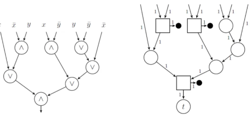
Figure 1The circuitCψ and the external-source flow gameGψ, forψ=x∨(¯x∧y)∧((x∧y¯)∨
(y∨y¯∨x¯)).
a thresholdγ∈IN, and the goal is to decide whethervalue(G)≥γ.
We show that the problem is complete in ΣP2, namely the class of problems that can be solved by a nondeterministic polynomial Turing machine that has an oracle to some NP-complete problem.
ITheorem 2. The FG problem is ΣP2-complete.
Proof. We start with the upper bound. Consider a flow game G and a threshold γ ∈IN. Strategies for Player 0 and Player 1 can be represented by polynomial-length strings. Given a strategy αfor Player 0, the problem of checking whether there is a strategyβ for Player 1 such thatoutcome(α, β)< γis in NP. Consequently, deciding whether there is a strategy α for Player 0 such that for every strategyβ for Player 1 we haveoutcome(α, β)≥γ, can be done by a nondeterministic polynomial-time Turing machine with an NP oracle.
We continue to the lower bound and describe a reduction from QBF2: satisfiability
for quantified Boolean formulas with 2 alternations of quantifiers, where the most ex-ternal quantifier is “exists". Letψ be a Boolean propositional formula over the variables x1, . . . , xn, y1, . . . , ym and let θ = ∃x1. . .∃xn∀y1. . .∀ymψ. Also, let X = {x1, . . . , xn},
¯
X ={¯x1, . . . ,x¯n}, Y ={y1, . . . , ym}, ¯Y ={¯y1, . . . ,y¯m},Z =X∪Y, and ¯Z = ¯X∪Y¯. We
construct a flow gameGθ such that the value ofGθ is 1 ifθ holds and is 0 otherwise.
We assume thatψis given in a positive normal form, that is,ψ is constructed from the literals in Z∪Z¯ using the Boolean operators∨ and∧, and that there isk ≥1 such that every literal inZ∪Z¯ appears in ψ exactlyk times. Clearly, every Boolean propositional formula can be converted with only a quadratic blow-up to an equivalent one that satisfies these conditions.
We first translate ψ into a Boolean circuit Cψ withk(2n+ 2m) inputs – one for each
occurrence of a literal in ψ. For example, in Figure 1, on the left, we describe Cψ for
ψ=x∨(¯x∧y)∧((x∧y¯)∨(y∨y¯∨x¯)). Each gate inCψ has fan-in 2 and fan-out 1. We
say that an input assignment to Cψ is consistent if it corresponds to an assignment to the
variables inZ. That is, for each variablez∈Z, there is a valueb∈ {0,1}such that all thek inputs that correspond to the literalzhave valueb and all thek inputs that correspond to the literal ¯zhave value ¯b. If the input to Cψ is consistent thenCψ computes the value ofψ
for the corresponding assignment.
Now, we translateCψ to anexternal-source flow gameGψ=hV0, V1, E, c, ti: a flow game
in which there is no source vertex, and an input flow is given externally. Formally, some of the edges inE have an unspecified source, to be later connected to edges with an unspecified
target. The idea behind the translation is as follows: The capacities inGψ are all 1. Each
OR gate inCψ induces a vertexv0in V0 that has in-degree 2 and out-degree 1. Thus, if the
incoming flow in each incoming edge tov0 is 0 or 1, then its outgoing flow is 1 iff at least one
of its incoming edges has flow 1. Then, each AND gate inCψ induces a vertexv1in V1 that
has in-degree 2 and out-degree 2, yet, one of the two edges that leavesv1 leads to a sink.
Accordingly, if the incoming flow in each incoming edge tov1 is 0 or 1, then the outgoing
flow in the edges that does not lead to the sink is 1 in all the policies forv1iff both incoming
edges have flow 1. For example, the Boolean circuitCψ from Figure 1 is translated to the
external-source flow gameGψ to its right.
The following lemma can be proved by an induction on the structure ofψ.
I Lemma 3. Consider a Boolean formula ψ and its corresponding external-source flow gameGψ.
1. Given input flows toGψ, if we increase some input flow, then the new value of the game
is greater than or equal to the original value.
2. Given input flows in {0,1} to Gψ, the value of the game is equal to the output ofCψ with
the same input. Thus, if the input flows to Gψ corresponds to a consistent input toCψ,
then the value ofGψ is the value ofψ for the corresponding assignment.
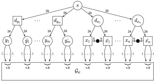
We complete the reduction by constructing the flow gameGθ, which usesGψas a sub-game.
As can be seen in Figure 2, the gameGθ has a source sthat can direct flow to a layer of
variable vertices– vertices associated with the variables inZ. The existentially quantified variables, namely these in X, are associated withV0 vertices, and the universally quantified
ones, namely these inY, are associated withV1vertices. The sourcescan direct 2kunits of
flow to each variable vertex. The third layer of the game consists ofliteral vertices: each variable vertexdz has two successors, associated with the literalszand ¯z. Vertices associated
with literals inX∪X¯ are inV1, whereas these associated with literals inY ∪Y¯ inV0. The edges from a variable vertex to its literal vertices have capacity 2k. Intuitively, the structure of the game, together with Lemma 3, imply that optimal strategies for both players directs all the 2k units that enter a variable vertexdz into one of its literal vertices, which corresponds
to a choice betweenzand ¯z. Consequently, there is a correspondence between the outgoing flow from the variable vertices and assignments to the variables, which induces an input to Cψ. Each outgoing edge from a literal vertex enters an input of Cψ that corresponds to this
literal.
In the full version we describe the gameGθ for the caseψ= (x∨y)∧(¯x∨y¯), and prove
that the value ofGθ is 1 ifθ holds and is 0 otherwise. J
Note that from the proof of Theorem 2 we can also conclude that the FG problem is ΣP
2-hard already for flow games in which the capacities of the edges are 1. Indeed, we can
change the reduction so that in the gameGθ, an edge with capacitydis replaced bydparallel
edges with capacity 1.
A natural question that arises is whether we can efficiently find an approximated solution for the FG problem. In particular, we say that a solutionxis a δ-approximation for the value of a flow gameG if x
δ ≤value(G)≤δ·x. As we now show, finding an approximated
solution to the FG problem is not easier than finding an exact solution. Formally, we have the following.
ITheorem 4. It isΣP2-hard to approximate the FG problem within any multiplicative factor. Proof. The reduction used for proving the ΣP
2 lower bound in the proof of Theorem 2 is
Figure 2The gameGθ.
whether the value of a flow game is 0 or 1 is already ΣP2-hard. Since every algorithm that approximates the solution of the problems within a multiplicative factor can determine whether the value of the game is positive or is 0, then approximated solution amounts to a precise solution, and is therefore ΣP
2-hard. J
3.1
Feasible Cases
We describe a variant of the problem as well as a structural restriction on games for which the FG problem can be solved efficiently.
Swallowing Flow. A most hostile environment is one that simply swallows all flow that reaches vertices it controls. That is, flow that reachesV1is lost. It is easy to analyze flow
games in this setting, as they coincide with traditional networks in which the vertices inV1
are eliminated. Indeed, Player 0 should avoid sending flow to vertices inV1. It follows that
maximal flow in this setting can be found in polynomial time. A variant of this setting is one in which there is a bound on the flow that Player 1 can swallow in each vertex. It is not hard to see that this variant can be reduced to our model by adding an edge to a sink from each vertex of Player 1. The capacity of the edge is the amount of flow that Player 1 can swallow in the vertex.
Tree Flow Games. Let G =hV0, V1, E, c, sibe a flow game without a target vertex. Let
V =V0∪V1. Assume that the directed graphhV, Eiis a tree, namely, the in-degree of every
vertex inV \ {s} is 1. The goal of Player 0 is to maximize the flow that enters the leaves of the tree. In the full version we show that if the out-degree of every vertex is bounded by a constant then the FG problem can be solved in polynomial time. Essentially, the value of a game from a vertexucan be expressed as a min-max expression over the possible values of the games that start from the successors ofu, which enables the formulation of the problem by means of dynamic programming. When the out-degrees of the vertices are constants, the latter can be solved in polynomial time.
4
No-Loss Flow Games
Recall that when the incoming flow is larger than the capacity of the outgoing edges, then flow is lost and the outgoing flow is lower than the incoming flow. Sometimes it is desirable to find a strategy of Player 0 such that for every strategy of Player 1, there is no loss of flow. We call such a strategy of Player 0 ano-loss strategy. Formally,α∈F0 is a no-loss strategy
if for every strategyβ∈F1, there is no vertexu∈V such that the flow that entersuinfα,β
is larger than the sum of the capacities of the edges that leaveu. Thus, for all verticesu∈V except forsandt, we haveP
e∈Euf
α,β(e) =P
e∈Eufα,β(e).
No-loss strategies are required in applications in which the authority cannot tolerate loss of traffic and is willing to reduce the flow in order to ensure no loss. For example, when it involves leaks of hazards or loss of crucial packets in a communication network. The trivial strategy, where the flow is 0, is clearly a no-loss strategy. In this section we study optimal no-loss strategies, namely no-loss strategies that ensure a maximal flow. Given a flow game G, letnl_value(G) denote the value of the Gwhen the strategy of Player 0 is restricted to strategies that ensure no loss.
Recall that in Theorem 2 we showed that deciding whethervalue(G)≥1 is ΣP
2-complete.
We start with some good news and show that if Player 0 is restricted to no-loss strategies, the problem can be solved in polynomial time. In order to prove this, we first definereachability games.
Consider a graphhV, Ei, source and target verticess, t∈V, and a partitionV0∪V1ofV.
The reachability game onhV0, V1, E, s, tiis played between Player 0 and Player 1 as follows.
Initially, a token is placed ons. Then, in each step, if the token is placed on a vertexu∈V0
(respectively,u∈V1), then Player 0 (respectively, Player 1) chooses a successor vertex v,
namelyvsuch thathu, vi ∈E, and moves the token tov. A strategy of Player 0 (respectively Player 1) maps each vertexu∈V0 (respectively, u∈V1) that is neithert nor a sink to a
successor vertexv. A pair of strategies,αfor Player 0 andβ for Player 1, induces a unique path, denoted outcome(α, β), to be traversed by the token when the players follow their strategies. When the graph is acyclic, the path is finite and Player 0 wins if the path reaches t. Otherwise, the path reaches a sink and Player 1 wins. Awinning strategy for Player 0 is a strategyαsuch that for every strategyβ of Player 1, the pathoutcome(α, β) reachest. it is well known that the problem of deciding the winner in a reachability game can be solved in linear time and is PTIME-complete [23].
ITheorem 5. Consider a flow gameG. Deciding whether nl_value(G)≥1can be done in linear time and is PTIME-complete.
Proof. We reduce the problem of deciding whether a flow game G = hV0, V1, E, c, s, ti
satisfies the requirement nl_value(G) ≥ 1 to the problem of deciding the reachability game G0 = hV
0, V1, E, s, ti, and reduce the reachability game for G0 to the problem of
deciding whether a flow gameG =hV0, V1, E, c, s, ti in which all capacities are 1 satisfies
nl_value(G) ≥ 1. The upper and lower bounds then follow from known complexity of reachability games. In both reductions, a no-loss strategy for Player 0 inG is related with a strategy for Player 0 inG0. Essentially, the successor vertex to which the flow of 1 is going to be directed in a no-loss strategy is the successor vertex to which the token is going to be moved, and vice versa. The details of the reductions can be found in the full version. J While deciding whether a positive outcome can be achieved by a no-loss strategy can be done in polynomial time, calculating the no-loss value of the game is not easier than in the
general case. Formally, in theno-loss flow game problem(NLFG problem, for short) the input is a flow gameG and a thresholdγ∈IN, and the goal is to decide whethernl_value(G)≥γ. ITheorem 6. The NLFG problem is ΣP
2-complete.
Proof. The upper bound is similar to the case where loss is allowed. Indeed, given a strategy αfor Player 0, the problem of checking whether there is a strategyβ for Player 1 such that there is loss or that outcome(α, β)< γ is in NP, which implies membership in ΣP
2 for the
NLFG problem.
For the lower bound, we show that the reduction from QBF2 described in the proof of
Theorem 2 can be manipulated to address no-loss strategies. Essentially, this is done by replacing all sinks by a single vertex in which loss is possible, but may be avoided when the formula is satisfiable. The details of the reduction are described in the full version. J
5
Non-Integral Flow Games
Recall that the capacities in the network are integral and that a policy for a vertex can assign only integral flows. Integral-flow games arise naturally in settings in which the objects we transfer along the network cannot be partitioned into fractions, as is the case with cars, packets, and more. Moreover, sometimes, as in cases of messages or other information packages, objects can be partitions up to a known granularity. It is easy to see that by multiplying all capacities by factorγ and solving an integer-flow game in the obtained game, we get a solution that involves strategies with fractions of 1
γ in the original game. Sometimes,
however, as in the case of liquids, flow can be partitioned arbitrarily. In the traditional one-player setting, it is known that when the capacities are integral, then there exists an integral maximum flows. In this section we study an extension of the setting and allow strategies to use flows in IR. We show that, interestingly, the game setting makes these strategies stronger, in the sense that partitioning outgoing flows into reals may enlarge the value of the game. Moreover, the gain cannot be bounded by a constant.
Consider a flow gameG=hV0, V1, E, c, s, ti. Let IR+ denote the set of non-negative real
numbers. Anon-integral policy for a vertexu6=sis a functionfu: IR+→IRE+u such that
for every flowx∈ IR+ and edge e∈Eu, we have fu(x)(e)≤c(e) and Pe∈Eufu(x)(e) = min{x,P
e∈Euc(e)}. Likewise, a non-integral policyfsfor the sourcesis a function in IR
Es
+ .
Thus, non-integral policies allow non-integral flows. We say that a strategy is anon-integral strategy if it contains non-integral policies. We useni_value(G) to denote the non-integral value ofG, namely the value when the players are allowed to use non-integral strategies. We first show that Player 0 can benefit from using non-integral strategies:
ITheorem 7. There is a flow gameG such that an optimal strategy for Player 0 in G must be non-integral even when Player 1 is restricted to integral strategies. Thus, ni_value(G)> value(G).
Proof. Consider the flow game appearing in Figure 3 on the left. Consider the non-integral strategyαthat assigns an outgoing flow of 2 tohs, uiand partitions the incoming flow to v0 equally between hv0, v1iandhv0, v2i. It is not hard to see that for every strategyβ for
Player 1, we have thatoutcome(α, β)≥1.5. Indeed, the sum of the incoming flows tov1 and
v2 is 2, implying that there is loss of flow in at most one of these vertices. Since the flow
fromv0 to bothv1 andv2 is at most 0.5, then the loss is at most 0.5. On the other hand,
if Player 0 is restricted to integral strategies, then an outcome of more than 1 cannot be ensured, as once Player 0 has chosen his strategy and directs 2 units tou, Player 1 can cause
Figure 3A FG in which Player 0 benefits from non-integral strategies (left) and its amplification (right).
a loss of 1 by choosing a policy inuthat directs 1 tov0and directs 1 to the vertex (v1orv2)
to which Player 0 directs the incoming flow of 1 tov0. J
In thenon-integral flow game problem(NIFG problem, for short) the input is a flow game Gand a threshold γ∈IR+, and the goal is to decide whetherni_value(G)≥γ. We consider
also theno-loss non-integral flow game problem (NLNIFG, somewhat shorter), where we consider non-integral strategies that also ensure no loss of flow.
The reduction from QBF2 described in Theorem 2 holds also for these new settings.
Indeed, by Lemma 3, the optimal strategies of the players would result in integral input to Gψ. Hence, the following theorem.
ITheorem 8. The NIFG and NLNIFG problems areΣP
2-hard. The NIFG problem is also
ΣP2-hard to approximate within any multiplicative factor.
Theorem 8 only gives a lower bound for the problem. The upper bound for the FG problem relied on the fact that integer strategies have a polynomial representation, which cannot be applied in the NIFG problem. Moreover, since reals are second-order creatures, the problem may be undecidable. We leave the decidability problem open and describe, in Section 6, a decidable variant. A natural question is whether an algorithm that solves the FG problem (for integral strategies) approximates the solution for the case of non-integral strategies. As we show in the following theorem, such an approximation cannot be bounded by a constant factor.
ITheorem 9. For alln >1, there is a flow gameGn s.t. value(Gn) = 1and ni_value(Gn)≥
n.
Proof. We amplify the construction used in the proof of Theorem 7. Recall that there, we showed that the flow game in Figure 3 on the left has value 1 and has non-integral value 1.5. The amplification involves two ideas: we parameterize the branching degree of v0 and we
use a recursion that involves sub-games for which a smaller ratio between the value and the non-integral value is known.
LetGbe a flow game such thatvalue(G) = 1 andni_value(G) =k, fork >1, and assume that 2kis an integer. For example, in the game presented in Figure 3 on the left, we have k= 1.5. We construct a flow gameG0 such thatvalue(G0) = 1 andni_value(G0) = 2k−1. By repeating the construction logarithmically many times, we obtain the required flow game Gn.
Consider the gameG. Let d1 andd2be the outgoing flow from the source in an optimal
thand1 andd2. We define the new gameG0 as shown in Figure 3 on the right. The gameG0
containsG twice as a sub-game: the incoming edge toG enters its source and the outgoing edge from G leaves its target. In a flow game on G0, the maximum flow to the vertex u that Player 0 can ensure with an integral strategy is 2. Hence, value(G0) = 1. Allowing non-integral strategies, the maximum flow to the vertexuthat Player 0 can ensure is 2k, makingni_value(G0) = 2k−1.
J
6
Dynamic Flow Games
In our definition of flow games, the players choose their strategies before the game starts. The universal quantification on the strategies of Player 1 implies that this is equivalent to a scenario in which Player 0 chooses a strategy and then Player 1 chooses a strategy. In dynamic flow games we refer to the way information flows in the graph and let the players choose policies in a vertex only after flow travels in the subgraph from which the vertex is reachable. Since the graph is acyclic, this is well defined.
Formally, we first order the graph in a topological ordering such thatV0 vertices appear,
whenever possible, beforeV1 vertices. That is, we fix a topological ordering≤such that if
there is neither a path from u∈V0 tov ∈V1 nor from v touthenu≤v. Now, Player 0
chooses a flow for each outgoing edge ofs. Then, we follow the order≤and for each vertex u, the player that controlsudirects the incoming flow to the outgoing edges. Thus, instead of choosing a strategy that describes the behavior for each possible incoming flow for each vertexu, the player just chooses how to direct the incoming flow, and he has information on the flow in edges whose source precedesuin ≤. The value of the game is the maximal flow tot that Player 0 can ensure.
Note that the dynamic setting is not equivalent to the non-dynamic (original) one. For example, the value of the flow game in Figure 3 is 1 (and is 1.5 when we allow non-integral strategies), whereas the dynamic setting leads to a value of 2. The flow game in Figure 3 suggests that the information about “earlier” flow helps Player 0 to use integral flows. Indeed, coming to decide the flow from vertexv0, Player 0 already known which ofv1and v2 have
already received 1 flow unit. As we show in the full version, however, the information may not be sufficient in general, and Player 0 can benefit from using non-integral strategies.
The ΣP
2 lower bounds described in Sections 3 and 4 apply also for the dynamic setting.
On the positive side, the dynamic setting enables a formulation of the problem by means of the first-order theories of integral addition or real addition, making the related decision problems decidable for both integral and real flows [15, 14].
7
Discussion and Future Work
Today’s computing environment involves parties that should be considered adversarial. This calls for a re-examination of classical algorithmic problems. We introduced and studied flow games, which capture settings in which the authority can control the flow only in part of the vertices in a flow network. Below we discuss possible extensions of our work as well as open problems we have left for future research.
7.1
Extensions
Evacuation. An evacuation flow game isG=h{s}, V1, E, c, s, ti. Thus, all vertices except
for the source belong to Player 1.4 As explained in Section 1, an evacuation flow game
corresponds to scenarios in which the authority has no control on how flow travels on the network [25]. Solving the FG problem in an evacuation flow game amounts to finding a strategy for Player 1 that minimizes the flow.
Beyond the clear practical applications, it is interesting to study the computational aspects of the evacuation problem. As it refers only to one player, and thus involves no alternation of quantification, there is hope the problem can be solved in polynomial time, possibly by a reduction to a prioritized variant of the maximal-flow problem. The latter is strongly related to several weighted variants of the max-flow problem. In particular, polynomial solutions are known for the min-cost max-flow problem [34] and to max-flow with lexicographically ordered edges problem [26].
A Classical Algorithmic Game-Theory Examination. Beyond the questions we studied for FGs, the game setting calls for a classical algorithmic game-theory examination: existence of a Nash equilibrium, stability inefficiency, and many more. We plan to study them for multiplayer flow games, where the vertices of the network are partitioned between somek >1 players, there arektarget vertices, and the objective of each player is to direct as much flow as possible to her target vertex. For example, in a communication network controlled by several companies (that is, vertices correspond to routers owned by the companies), each company wants to maximize the number of messages from its source to target vertices, and we want to find the best Nash equilibria or design networks for which this equilibria is close to the social optimum.
Partially Specified Networks. In some cases, a strategy is known for some vertices and we need to find an optimal strategy for the others. For example, in hybrid networks, where some vertices are new SDN routers whose behaviour can be controlled, and the other vertices run known traditional routing protocols (e.g., route via the shortest path) [3]. As another example, consider the case where each time that a driver reaches an uncontrolled vertex, it randomly chooses an outgoing edge with free capacity. In this case, we need to find a strategy that maximizes the expected flow to the target.
7.2
Open Problems
Recall that a maximum flow in a flow game may involve non-integrals even when all capacities are integrals. While we settle the complexity of flow games for strategies that only use integrals, decidability for the setting in which strategies may use non-integrals is open. One approach to obtain decidability and analyze flow games with non-integral strategies is to approximate their value with integral strategies. While such an approximation cannot be bounded by a constant multiplicative factor (Theorem 9), we conjecture that it can be bounded by a linear additive factor. In particular, we conjecture that for every flow game G, we have that ni_value(Gn)≤value(Gn) +|E|, where the intuition is that a non-integral
4 Recall that we define a flow game withs∈V0. Alternatively, we could have defined an evacuation flow
game as one in which all vertices are inV1and parameterize the game with an initial flow that enterss. Indeed, saturating the edges fromsis a dominating strategy for Player 0, so Player 0 does not really take decisions even whens∈V0.
flow in Gshould not exceed flow in the game obtained from Gby increasing all capacities by 1. Another approach would be to find a granularity to which it would be sufficient to break an integral flow. Our efforts in this direction so far reveal some counter-intuitive facts. For example, flow games are notlocal monotonic: increasing the flow that enters a vertex may cause a decrease in the flow directed by an optimal strategy to one of its outgoing edges. Also, the required granularity is not continuous, in the following sense: for every k≥1, we can generate a FG such that an optimal strategy that can break the flow into the fractions 12,13, . . . ,k−11 achieves the same flow achieved by an optimal strategy that only uses integrals, yet breaking the flow into the fraction k1 improves this flow. Also, while we know that non-integral strategies may be better than integral ones, we do not know whether strategies that use rational numbers are as good as strategies that use real ones.
Acknowledgment. We thank David Hay for helpful discussions on software-defined net-works.
References
1 S. Agarwal, M. S. Kodialam, and T. V. Lakshman. Traffic engineering in software defined networks. In Proc. 32nd IEEE International Conference on Computer Communications, pages 2211–2219, 2013.
2 R.K. Ahuja, T.L. Magnanti, and J.B. Orlin. Network flows: Theory, algorithms, and applications. Prentice Hall Englewood Cliffs, 1993.
3 B. Aminof, O. Kupferman, and R. Lampert. Rigorous approximated determinization of weighted automata. Theoretical Computer Science, 480:104–117, 2013.
4 E. Anshelevich, A. Dasgupta, J. Kleinberg, E. Tardos, T. Wexler, and T. Roughgarden. The price of stability for network design with fair cost allocation. SIAM J. Comput., 38(4):1602–1623, 2008.
5 T. Bartnicki, J. A. Grytczuk, H. A. Kierstead, and X. Zhu. The map coloring game. AmericanMathematical Monthly, 114:793–803, 2007.
6 A.K. Chandra, D.C. Kozen, and L.J. Stockmeyer. Alternation. Journal of the Association for Computing Machinery, 28(1):114–133, 1981.
7 S.A. Cook. Path systems and language recognition. InProc. 2nd ACM Symp. on Theory of Computing, pages 70–72, 1970.
8 S.A. Cook. The complexity of theorem-proving procedures. InProc. 3rd ACM Symp. on Theory of Computing, pages 151–158, 1971.
9 T.H. Cormen, C.E. Leiserson, and R.L. Rivest.Introduction to Algorithms. MIT Press and McGraw-Hill, 1990.
10 E.A. Dinic. Algorithm for solution of a problem of maximum flow in a network with power estimation.Soviet Math. Doll, 11(5):1277–1280, 1970. English translation by RF. Rinehart. 11 J. Edmonds and R.M. Karp. Theoretical improvements in algorithmic efficiency for network
flow problems. Journal of the ACM, 19(2):248–264, 1972.
12 S. Even, A. Itai, and A. Shamir. On the complexity of timetable and multicommodity flow problems. SIAM Journal on Computing, 5(4):691–703, 1976.
13 J. Feigenbaum, C.H. Papadimitriou, R. Sami, and S. Shenker. A BGP-based mechanism for lowest-cost routing. Distributed Computing, 18(1):61–72, 2005.
14 J. Ferrante and C. Rackoff. A decision procedure for the first order theory of real addition with order. SIAM Journal on Computing, 4(1):69–76, 1975.
15 M.J. Fischer and M.O. Rabin. Super-exponential complexity of presburger arithmetic. In Quantifier Elimination and Cylindrical Algebraic Decomposition, pages 27–41, 1974.
16 L.R. Ford and D.R. Fulkerson. Maximal flow through a network. Canadian journal of Mathematics, 8(3):399–404, 1956.
17 L.R. Ford and D.R. Fulkerson. Flows in networks. Princeton Univ. Press, Princeton, 1962. 18 Z. Füredi, D. Reimer, and A. Seress. Triangle-free game and extremal graph problems.
Congressus Numerantium, 82:123–128, 1991.
19 A.V. Goldberg, É. Tardos, and R.E. Tarjan. Network flow algorithms. Technical report, DTIC Document, 1989.
20 A.V. Goldberg and R.E. Tarjan. A new approach to the maximum-flow problem. Journal of the ACM, 35(4):921–940, 1988.
21 D. Hefetz, M. Krivelevich, A. Naor, and M. Stojaković. On saturation games. European Journal of Combinatorics, 41:315–335, 2016.
22 D. Hefetz, O. Kupferman, A. Lellouche, and G. Vardi. Spanning-tree games. To appear, 2018.
23 N. Immerman. Number of quantifiers is better than number of tape cells. Journal of Computer and Systems Science, 22(3):384–406, 1981.
24 E. Kalai and E. Zemel. Totally balanced games and games of flow. Mathematics of Opera-tions Research, 7(3):476–478, 1982.
25 S. Keren, A. Gal, and E. Karpas. Goal recognition design for non optimal agents. InProc. 29th AAAI conference, pages 3298–3304, 2015.
26 D. Kozen. Lexicographic flow. Technical Report http://hdl.handle.net/1813/13018, Com-puting and Information Science, Cornell University, June 2009.
27 O. Lichtenstein and A. Pnueli. Checking that finite state concurrent programs satisfy their linear specification. InProc. 12th ACM Symp. on Principles of Programming Languages, pages 97–107, 1985.
28 N. Nisan, T. Roughgarden, E. Tardos, and V.V. Vazirani. Algorithmic Game Theory. Cambridge University Press, 2007.
29 M. J. Osborne and A. Rubinstein. A Course in Game Theory. The MIT Press, 1994. 30 A. Pnueli and R. Rosner. On the synthesis of a reactive module. InProc. 16th ACM Symp.
on Principles of Programming Languages, pages 179–190, 1989.
31 L. Qingsong, G. Betsy, and S. Shashi. Capacity constrained routing algorithms for evacu-ation planning: A summary of results. InInternational Symposium on Spatial and Temporal Databases, pages 291–307. Springer, 2005.
32 B.L. Schwartz. Possible winners in partially completed tournaments. SIAM Review, 8(3):302–308, 1966.
33 L.J. Stockmeyer. On the combinational complexity of certain symmetric boolean functions. Mathematical Systems Theory, 10:323–336, 1977.
34 É. Tardos. A strongly polynomial minimum cost circulation algorithm. Combinatorica, 5(3):247–255, 1985.
35 S. Vissicchio, L. Vanbever, and O. Bonaventure. Opportunities and research challenges of hybrid software defined networks. Computer Communication Review, 44(2):70–75, 2014.