Learning Program-Wide Code Representations for Binary Diffing

UC Riverside

UC Riverside Electronic Theses and Dissertations

Title

Learning Program-Wide Code Representations for Binary Diffing

Permalink

Author

Publication Date

License

UNIVERSITY OF CALIFORNIA RIVERSIDE

Learning Program-Wide Code Representations for Binary Diffing

A Thesis submitted in partial satisfaction of the requirements for the degree of

Master of Science in Computer Science by Xuezixiang Li March 2019 Thesis Committee:

Dr. Heng Yin, Chairperson Dr. Chengyu Song

Copyright by Xuezixiang Li

The Thesis of Xuezixiang Li is approved:

Committee Chairperson

Acknowledgments

First of all, I would like to give my sincere gratitude to my advisor, Prof. Heng Yin, with out whose guidance, I could not finish the thesis. Second, I am grateful to the committee members Prof. Chengyu Song and Prof. Zhiyun Qian. Your suggestions and comment play a significant role during this period. Thanks for your help. I also appreciate Yue Duan and other group members in our lab. I appreciate all of your suggestions ideas and assistance for this project. Besides, I am particularly grateful for the guidance given by Prof. Dan Chen from Wu Han University, which starts my journey of scientific research. Last but not foremost, I wish to thank my parents and girlfriend for their support and encouragement throughout my study.

ABSTRACT OF THE THESIS

Learning Program-Wide Code Representations for Binary Diffing

by

Xuezixiang Li

Master of Science, Graduate Program in Computer Science University of California, Riverside, March 2019

Dr. Heng Yin, Chairperson

Binary diffing analysis quantitatively measures the differences between two given binaries and produces fine-grained basic block matching. It has been widely used to en-able different kinds of critical security analysis. However, all existing program analysis and learning based techniques suffer from low accuracy, poor scalability, coarse granularity espe-cially on COTS binaries which did not contains complete debug information. On the other hands, some learning based approaches require extensive labeled training data to function, so that precise labelled and representative dataset is needed to obtain great results. To surmount such limitations, in this paper, we come up with a novel learning based code representation generation approach to solve the binary diffing problem. We rely only on the code semantic information as well as the program-wide control flow structural information to generate block embeddings without supporting of any debug information. Furthermore, we propose a K-hop greedy matching algorithm to find the optimal diffing results using the generated block representations. We implement a prototype called DeepBinDiff and evaluate its effectiveness and efficiency with large number of binaries and real-world

vul-nerabilities. The results show that our tool could outperform the state-of-the-art binary diffing tools by large margin for both cross-version and cross-optimization level diffing. A case study for OpenSSL using real-world vulnerabilities further demonstrates the usefulness of our system.

Contents

List of Figures x

List of Tables xi

1 Introduction 1

2 Related Work 7

2.1 Code Similarity Detection . . . 7

2.2 Assembly code processing . . . 10

2.3 Graph mining . . . 11 3 Problem Statement 13 3.1 Problem Definition . . . 13 3.2 Assumptions . . . 14 4 System Design 16 4.1 Approach Overview . . . 16 4.2 Pre-processing . . . 17 4.2.1 CFG Generation . . . 18

4.2.2 Feature Vector Generation . . . 18

4.3 Embedding Generation . . . 26

4.3.1 TADW algorithm . . . 26

4.3.2 Graph Merging . . . 27

4.3.3 Basic Block Embeddings . . . 29

4.4 Code Diffing . . . 30

4.4.1 K-Hop Greedy Matching . . . 32

5 Evaluation 33 5.1 Experimental Setup . . . 33

5.2 Implementation . . . 34

5.3 Datasets & Baseline Techniques . . . 35

5.3.1 Datasets. . . 35

5.4 Ground Truth Collection . . . 36

5.5 Effectiveness . . . 38

5.5.1 Evaluation Metrics . . . 38

5.5.2 Cross-version Diffing . . . 40

5.5.3 Cross-optimization level Diffing . . . 42

5.6 Efficiency . . . 43

5.7 Case Study . . . 44

5.7.1 DTLS Recursion Flaw . . . 44

5.7.2 Memory Boundary Checking Failure . . . 46

6 Discussion 48 7 Conclusions 50 Bibliography 51 .1 Cross-version Binary Diffing F1-score CDF Figures . . . 56

List of Figures

4.1 Overview of DeepBinDiff. . . 17

4.2 Token Embedding Model Generation. . . 20

4.3 Token2Vec model used in DeepBinDiff . . . 25

4.4 TADW . . . 28

4.5 Graph Merging . . . 29

5.1 Matching for DTLS Recursion Flaw . . . 46

5.2 Matching for Memory Boundary Checking Failure . . . 46

.1 Cross-version Diffing F1-score CDF for Coreutils . . . 56

List of Tables

4.1 Basic block features in Gemini[60] . . . 18

5.1 Hyper Parameter selection . . . 35

5.2 Experimental Datasets . . . 38

5.3 Cross-version Binary Diffing Results . . . 41

Chapter 1

Introduction

Binary Code Differential Analysis, a.k.a, binary diffing, is a fundamental analysis capability, which aims to quantitatively measure the similarity between two given binaries and produce the fine-grained block level matching. Given two input binaries, it precisely characterizes the program-wide differences by generating the optimal matching among the blocks with quantitative similarity scores. It can not only present a more precise, fine-grained and quantitative results about the differences at a whole binary scale but also explicitly reveal how code evolves across different versions or optimization levels. Due to this level of precision and granularity, it has enabled many critical security usages in differ-ent scenarios when program-wide analysis is required, such as changed parts locating [2], malware analysis [29, 49], patch analysis [61, 42], binary wide plagiarism detection [45] and patch-based exploit generation [13].

Because of the importance, binary diffing has been an active research focus. Bin-Diff [9] which is the state-of-the-art commercial binary diffing tool performs many-to-many

graph isomorphism detection on callgraph and control-flow graph (CFG) and leverages heuristics (e.g., function name hash, graph edge MD index) to match functions as well as blocks. Other techniques perform diffing on the generated flow graphs [26, 55, 28] or de-compose the binaries into fragments [24, 22, 23] for similarity detection. These approaches do not consider the semantics of instructions which can be critical during analysis, espe-cially when dealing with different compiler optimization levels. Moreover, traditional graph matching algorithm such as Hungarian algorithm [39] is expensive and cannot guarantee optimal matching.

Another line of research utilizes dynamic analysis for diffing. These techniques carry out the analysis by directly executing the given code [27, 59], performing dynamic slicing [48] or using symbolic execution [31, 47, 45] on the given binaries and checking the semantic level equivalence based on the information collected during the execution. In general, these techniques excel at extracting semantics of the code and have good resilience against compiler optimizations and code obfuscation but usually suffer from very poor scalability and incomplete code coverage because of the nature of dynamic analysis.

Recently, researchers have been leveraging the advance of machine learning to tackle the problem. Various techniques such as Genius [30], Gemini [60], INNEREYE [64] and Asm2Vec [25] have been proposed to utilize graph representation learning techniques [21, 46, 41] and incorporate code information into embeddings (i.e, high dimensional numerical vectors). Then they use these embeddings for similarity detection. INNEREYE [64] and Asm2Vec [25] further leverage NLP techniques to automatically extract semantic informa-tion and generate embeddings for diffing.

These approaches embrace multiple advantages over the traditional static and dynamic approaches: 1) higher accuracy as they incorporate unique features of the code into the analysis by using either manual engineered features [30, 60] or deep learning based automatic methods [25, 64]; 2) better scalability since they avoid heavy graph matching algorithm or dynamic execution. Moreover, the deep learning process can be significantly accelerated by GPUs.

Limitations to Existing Learning based Techniques. Despite the advantages, we identify three major limitations for the existing learning based approaches.

First, no existing technique can perform program-wide binary diffing at a fine-grained basic block level. They either perform diffing on functions [30, 60, 40, 25] or on small code components [64], and tells how two given functions or small pieces of blocks are similar. As mentioned above, fine-grained binary diffing is an important analysis upon which many critical security analysis can be built. Hence, a more fine-grained binary diffing tool is strongly desired. And we argue that current existing code components search techniques is hard to extend to perform a program-wide fine-grind binary diffing problem. First, most of the approaches are only able to perform function level comparison which is not enough for fine-grind binary diffing. Second, low false positive is required in such task. Assuming that two functions A and B are mistakenly matched, the original target A0 would be possibly matched to another function C. Once C has another original target C0, the false positive will be propagated continuously.

Second, none of them considers both program-wide dependency information as well as basic block semantic information during analysis. INNEREYE [64] extracts block

semantic information with NLP techniques [46] but only considers local control dependency information within a small code component by adopting the Longest Common Subsequence (LCS). Asm2Vec [25] generates multiple random walks within functions and uses the walks to learn token and function embeddings. It is especially troublesome when performing binary diffing as one binary could contain multiple very similar functions. In this case, program-wide function calling relations can be vital in differentiating these functions.

Third, most of the learning based techniques [61, 40, 64] are based on supervised learning. Thus, the performance is heavily dependent on the quality of training data. We argue that a large, representative and balanced training dataset can be very hard to collect in binary diffing problem due to the extreme diversity of the binary programs.

Our Approach. To this end, we propose an unsupervised deep neural network (DNN) based program-wide code representation learning technique for binary diffing. In partic-ular, our technique learns basic block level embeddings for binary diffing via completely unsupervised learning. Each learned embedding represents a specific block by carrying not only the semantic information of the block but also the structural information from the program-wide inter-procedural control flow graph (ICFG). These embeddings are used to efficiently and accurately calculate the similarities.

To achieve this, we leverage NLP techniques to generate token (opcode and operands) embeddings which are further averaged and concatenated to assemble block level feature vectors. These feature vectors contain the semantic information for specific blocks. Then, we merge the two ICFGs of the input binaries on selected terminal nodes (no outgoing edge) so that the merged graph contains program-wide structural information for both

bi-naries yet the original dependency information remains unchanged. Matrix factorization is then performed on the graph along with the generated feature vectors to produce block level embeddings using Text-associated DeepWalk algorithm (TADW) [62]. Consequently, these block embeddings contain both the program-level structural information as well as the semantics from the blocks. Finally, to deal with the unique challenge of binary diff-ing, we present a K-hop greedy matching algorithm to match blocks and confront compiler optimizations including function inlining, instruction reordering, etc.

We implement a prototype named DeepBinDiff and conduct an extensive evalua-tion with three representative datasets containing 113 binaries. The evaluaevalua-tion results show that our tool outperforms the state-of-the-art tools BinDiff and Asm2Vec by large margin in terms of effectiveness with respect to cross-version and cross-optimization level diffing. Furthermore, we also conduct a case study using real-world vulnerabilities in OpenSSL [8]. The case study also shows that our tool has unique advantages when analyzing vulnerabili-ties. To our best knowledge, our evaluation is the only work that comprehensively examines the cross-version and cross-optimization binary diffing problem.

Contributions. In summary, the contributions of this paper are as follows:

• We propose a novel unsupervised program-wide code representation learning technique for binary diffing. Our technique rely on both the code semantic information as well as the program-wide control-flow graph structural information to generate high quality block embeddings. Then a K-hop greedy matching algorithm is proposed to obtain the optimal diffing results.

• We implement a prototype DeepBinDiff. It first extracts semantic information by leveraging NLP (Neutral Language Processing) technique. Then, it performs Text-associated DeepWalk algorithm to generate block embeddings that contain both the semantic and the inter-procedural control-flow information. The generated embed-dings are used to perform binary diffing with the help of K-hop greedy matching algorithm.

• An extensive evaluation shows that DeepBinDiff could outperform the state-of-the-art binary diffing tools by large margin for both cross-version and cross-optimization level diffing. A case study further demonstrates the usefulness of DeepBinDiff with real-world vulnerabilities.

Chapter 2

Related Work

In this section, we survey some related work about code similarity detection, As-sembly code processing and graph mining.

2.1

Code Similarity Detection

As mentioned, the existing code similarity search technique falls into three cate-gories: static analysis, dynamic analysis and learning based approaches.

Static Approaches Static approaches transform binary code into graphs (e.g., control flow graph) using program static analysis and then perform the comparison among binary code. Bindiff [9, 26] which is the state-of-the-art binary diffing commercial tool, performs many-to-many graph isomorphism detection on callgraph to match functions and leverages intra-procedural CFG graph matching for basic blocks. Considering for the efficiency, the tool rely on some heuristics (may not be available in stripped binaries) including name hashing, constant strings, edge counts, etc. Different rules are assigned different priority and

perform iteratively. Binslayer [15] further augments the graph matching with the Hungarian algorithm for bipartite graph matching to improve the matching results. Pewny et.al. [55] searches bugs within binary programs by collecting a list of input/output pairs to capture the semantics of a basic block and perform graph matching. The major drawback for graph matching based approaches is that the algorithms in general is very expensive. For the sake of improving runtime performance, discovRE [28] chooses to use lightweight syntax level features and applies pre-filtering before graph matching. However, the pre-filtering process may significantly affect the accuracy of the matching result [30].

Due the limitations of graph matching, techniques are proposed to use static pro-gram analysis to decompose functions into fragments. Tracelet [24] converts CFGs into a number of paths with fixed-length called Tracelets and then matches them by rewriting. Esh [22] decomposes the functions into segments named strandswhich represent data-flow dependencies and uses statistical reasoning to calculate similarities. GitZ [23] further im-proves Esh to find strands equality through re-optimization. Although no heavy graph matching is required, these techniques still bear with two major limitations. First, to ab-stain from massive number of fragments, they can only decompose within functions. Second, these techniques can not handle instruction and basic block reordering.

Dynamic Approaches Based on an insight that similar code must have semantically similar behavior, dynamic analysis becomes another promising line of research. Blanket Execution [27] executes functions of the two input binaries with the same inputs and com-pares monitored behaviors for similarity. BinHunt [31] uses symbolic execution and theorem proving and compares intra-procedural CFGs to find the matching between basic blocks.

iBinHunt [47] extends the comparison to inter-procedural CFGs and reduces the number of candidates of basic block matching by monitoring the execution under a common in-put. CoP [45] also uses symbolic execution to compute the semantic similarity of blocks and leverages the longest common sub-sequence of linearly independent paths to measure the similarity. BinSim [48] which is specifically proposed to compare binaries with code obfuscation techniques, relies on system calls to perform dynamic slicing and then check the equivalence with symbolic execution. Essentially, dynamic analysis approaches could deliver accurate results when facing compiler optimizations or even obfuscation. However, dynamic analysis based approaches by nature suffer from poor scalability and incomplete code coverage problem.

Learning Based Approaches Recently, researchers have turned to machine learning techniques to detect code similarity. Genius [30] forms attributed control flow graphs (ACFG) for each function and calculates the similarity through their graph embeddings which are generated through comparing with a set of representative ACFGs named code-book. Gemini [60] directly improves Genius by leveraging neural network to generate em-beddings for each binary function. Then it trains a Siamese network for similarity detection. INNEREYE [64] regards instructions as words and basic blocks as sentences and utilizes LSTM-RNN to automatically encode the information of basic blocks and further uses a Siamese network to detect the similarity. Both Gemini and INNEREYE rely on super-vised learning and requires extensive training with massive labeled training dataset. And both approaches is hard to handle different code obfuscation techniques and compile time code optimization without being trained by datasets that processed by such techniques.

Asm2Vec [25] adopts an unsupervised learning approach by generating token and function embeddings using PV-DM model. However, it only works on function comparison but can-not perform binary diffing at more fine-graind basic block level. Also, it does can-not consider any program-wide CFG structural information during analysis. PV-DM, as an old-school Neutral Language Processing (NLP) model can only capture unique keywords set from a given function instead of finding out real semantic meaning of each code sequence.

2.2

Assembly code processing

Nowadays, because of characteristic shared by both neutral languages and as-sembly code, researchers started to use Neutral Language Processing (NLP) techniques to process assembly languages. For instance, INNEREYE [64] and another approach [14] try to use Word2Vec as a pre-processing model to generate instruction embeddings. And on the top of instructions, some approaches [64, 25] uses RNN-LSTM and Doc2Vec model to deal with code sequences. Dislike troditional neural language articles, binaries also con-tain structural information such as data dependencies and control flows. There are two different methods to solve such problem. The fist is to adopt RandomWalk [25] to serialize control-flow graphs. The other way is to use a single model such as LSTM [64] and let the model itself to find inner structure information without recovering any control flow or data dependence information.

2.3

Graph mining

Graph analysis has been increasingly popular as many problems can be modeled as graphs. Generating vector representation of each node which contains important graph and node properties, a.k.a, graph embedding learning, has become widely popular. There are two different way to capture structural information and node features, which is traditional matrix factorization and Deep learning based method.

Matrix Factorization Ahmed et.al. [12] proposes a graph factorization technique to fac-torizes the adjacency matrix of the input graph by minimizing a loss function. GraRep [18] defines a node transition probability and proposes a k-order proximity preserved embedding method. The major drawback is scalability. HOPE [52] is similar to GraRep and preserves higher-order proximity. It fully captures transitivity and uses generalized Singular Value Decomposition to perform efficiently. DeepWalk [54] is proposed to learn latent represen-tations of nodes in a graph using local information from truncated uniform random walks. And node2vec [33] specifically designs a biased random walk procedure that efficiently ex-plores diverse neighborhoods of a node to learn continuous feature representations of nodes. These two model are based on random walk and have a Word2Vec model built top of the walkers. The main difference between those two approaches is the search strategies. In DeepWalk, walkers use Deep-First search (DFS) to pick new successors, while walkers in node2vec, combines deep first search (DFS) and Breadth-First search (BFS) to choose the next target vertex. And both has been proved to be equivalent with the factorization on adjacency matrices [62]. TADW [62] is the technique leveraged by DeepBinDiff, the major

advantage is that it considers feature vectors for nodes during matrix factorization. A re-cent work REGAL [34] is proposed to perform matrix factorization very efficiently with the consideration of node features. However, it only checks the existence of features other than considering the numeric values.

Deep Learning. DNGR [19] proposes a novel graph representation model based on deep neural networks that can capture the graph structure information directly. SDNE [58] de-signs a semi-supervised deep model that has multiple layers of non-linear functions to cap-ture both the local and global graph struccap-ture that is highly non-linear. GCN [37] uses a lo-calized first-order approximation of spectral graph convolutions to perform semi-supervised learning on graphs in a scalable way. Structure2Vec [21] is proposed for structured data representation via learning features spaces that embeds latent variable models.

Chapter 3

Problem Statement

In this section, we formalize the problem definition for binary diffing problem and further describe our problem statement and design goals.

3.1

Problem Definition

Given two binary programs, binary diffing precisely measures the similarity and characterizes the differences between the two binaries at a fine-grained basic block level. We formally definebinary diffing problem as follows:

Definition 1. Given two binary programsp1 = (B1, E1) and p2 = (B2, E2), binary diffing

aims to find the optimal block match combinationM(p1, p2) that maximizes the similarity

betweenp1 and p2: SIM(p1, p2) = argmax

m1,m2,...,mk∈M(p1,p2) mi∈M(p1,p2) X sim(mi), where: • B1 = {b1, b2, ..., bn} and B2 = {b 0 1, b 0 2, ..., b 0

n} are two sets containing all the basic

• Each element e in E ⊆B ×B corresponds to control flow dependency between two basic blocks;

• Each elementmi inM(p1, p2) represents a matching pair between bi and b

0

i;

• sim(mi) defines the quantitative similarity score between two matching basic blocks.

Therefore, the problem can be transformed into two subtasks: 1) introducing sim(mi) which quantitatively measures the similarity between two basic blocks; 2) finding

the optimal matching between two sets of basic blocks M(p1, p2).

3.2

Assumptions

To formalize our problem domain, we list the following assumptions on the given inputs:

• Only stripped binaries are given. This assumption in general makes the problem harder as no source or symbol information is presented. However, this assumption is very realistic as COTS binaries are often stripped and malware binaries do not carry internal symbols for obvious reasons.

• Binaries are not packed but can be optimized with different compiler optimization levels. Different optimization levels can result in distinctive binary codes even with the same source code input. Tolerating differences in binaries introduced by optimization levels is also very important to the code diffing problem. From the evaluation we can see that even the state-of-the-art tools cannot handle them well. So for packed

malware binaries, we assume they are unpacked by using existing unpacking tools before being present to our tool.

• Two input binaries are for the same architecture. So far DeepBinDiff supports x86 binaries since they are the most prevalent in real world binaries. Of course, DeepBin-Diff could be extended to handle cross-architecture diffing by performing analysis on an Intermediate Representation (IR) level. We leave it as future work.

Chapter 4

System Design

4.1

Approach Overview

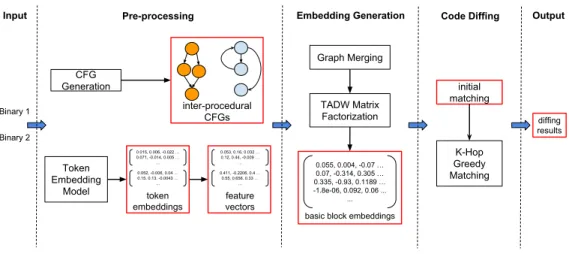
Figure 4.1 delineates the system architecture of DeepBinDiff. In this figure, the squares with red border is some intermediate data generated my different components of the system. The system can be divided into three main components: Pre-processing, Embed-ding Generation and Code Diffing. As shown in the figure, the system take two binaries as inputs. The pre-processing part is responsible for preparing input data for next component. Firstly, we disassemble the binary and recover assembly instructions and control-flow graph. The assembly instruction is used to generate feature vectors of each basic block. Feature vectors and Control-flow graph are taken as input of the TADW [62] in second component. Then the TADW model will generate embeddings for each basic block. Next, in the third component, those embeddings is compared and a K-Hop Greedy Matching algorithm is per-formed based on the result of comparison. This algorithm will generate a matching result

Binary 1 Binary 2 CFG Generation Token Embedding Model Input 0.015, 0.006, -0.022 … 0.071, -0.014, 0.005 … ... 0.052, -0.006, 0.04 … 0.15, 0.13, -0.0043 … ...

Pre-processing Embedding Generation

0.055, 0.004, -0.07 … 0.07, -0.314, 0.305 … 0.335, -0.93, 0.1189 … -1.8e-06, 0.092, 0.06 ... ... K-Hop Greedy Matching Code Diffing token embeddings TADW Matrix Factorization

basic block embeddings 0.053, 0.16, 0.032 … 0.12, 0.44, -0.009 … ... 0.411, -0.2206, 0.4 … 0.55, 0.656, 0.33 … ... feature vectors inter-procedural CFGs Output diffing results Graph Merging initial matching

Figure 4.1: Overview of DeepBinDiff.

M(p1, p2) which is the output of our system.

In section 4.2, we will introduce the pre-processing phase. We will also introduced how to recover inter-procedure and generate feature vector for basic blocks. In section 4.3, we will introduce some detail of TADW and how DeepBinDiff take it into use. In section 4.3, we will introduce how to perform code diffing and generate matching pairs based on K-Hop Greedy algorithm.

4.2

Pre-processing

In this phase, we generate two kind of data for TADW model, which is inter-procedural CFG and preliminary feature vectors of basic blocks. Here we capture the semantic features from the basic blocks and generate vectors based on such features.

Table 4.1: Basic block features in Gemini[60]

Type Feature Name

Block-level features

String Constants Numeric Constants

Number of Transfer Instructions Number of Function Calls Number of Instructions

Number of Arithmetic Instructions Inter-block features Number of offspring

Betweenness

4.2.1 CFG Generation

By combining call graph of the binary with control-flow graphs of each function, inter-procedural CFG (ICFG) contains control dependency information among basic blocks cross function boundaries. ICFG in DeepBinDiff plays a very important role, that is to provide program-wide contextual information when calculating block similarities. This in-formation is particularly useful when there exist multiple semantically similar blocks. In this case, this contextual information can be of great help in differentiating them. However, none of the existing techniques assimilate this information for binary diffing. DeepBinDiff leverages [1] to extract basic block information and generates inter-procedural CFGs for the two given binaries.

4.2.2 Feature Vector Generation

Besides the structural control dependency information carried by ICFGs, Deep-BinDiff also takes into account the semantic information from basic blocks by generating feature vector for each block.

Existing techniques such as Genius [30] and Gemini [60] empirically select some features from basic blocks and control flow graphs and then embed them into the CFGs to form attributed CFGs (ACFG). An example has been shown in table 4.1. However, by manually selecting limited number of features, one could easily miss some essential infor-mation and impose bias to the results. Furthermore, once attackers have gained access to details of the model and leaked such information, it is easy to come up with attacks aiming at these manually selected features. To overcome this limitation, INNEREYE [64] takes a supervised learning approach, utilizes Word2Vec to generate instruction embeddings and further deploys an LSTM-RNN model to convert instruction embeddings to block embed-dings. It requires sizable and balanced training dataset with labels (which can be hard to extract) to train the LSTM model. Asm2Vec [25], on the other hand, uses an unsupervised PV-DM model to produce the token and function embeddings. In DeepBinDiff, we take the unsupervised learning approach as well due to the fact that labels and balanced training dataset can be very hard to generate in binary diffing scenario.

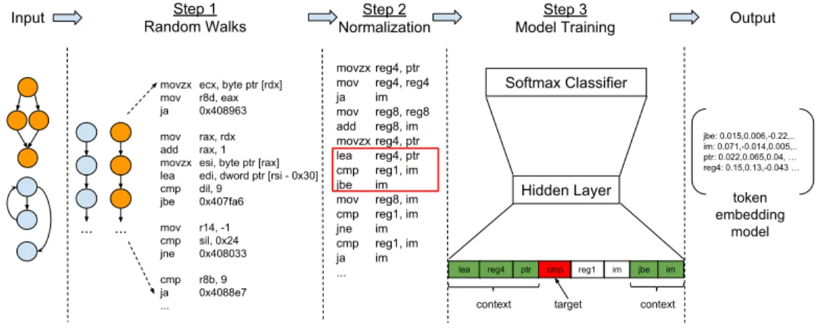
In DeepBinDiff, we leverage an unsupervised NLP technique Word2Vec [46] model which can generate embeddings for each word based on its context (words around it) to extract the semantics of each block. In our case, we consider each token (opcode or operand) as word, generate random walks on top of ICFGs to be sentences and instructions around each token as its context. More details will be shown in Model Training section later.

The whole process consists of two subtasks: token embedding generation and feature vector generation. More specifically, we first train a token embedding model using Word2Vec, then use this model to generate token embeddings. These token embeddings

jbe: 0.015,0.006,-0.22,.. im: 0.071,-0.014,0.005,.. ptr: 0.022,0.065,0.04, … reg4: 0.15,0.13,-0.043 … token embedding model Step 1 Random Walks Step 2 Normalization Step 3

Model Training Output

movzx reg4, ptr mov reg4, reg4 ja im mov reg8, reg8 add reg8, im movzx reg4, ptr lea reg4, ptr cmp reg1, im jbe im mov reg8, im cmp reg1, im jne im cmp reg1, im ja im ... ... ...

movzx ecx, byte ptr [rdx] mov r8d, eax

ja 0x408963

mov rax, rdx add rax, 1 movzx esi, byte ptr [rax] lea edi, dword ptr [rsi - 0x30] cmp dil, 9 jbe 0x407fa6 mov r14, -1 cmp sil, 0x24 jne 0x408033 cmp r8b, 9 ja 0x4088e7 ... ...

lea reg4 ptr cmp reg1 im jbe im

context target context

Hidden Layer Softmax Classifier Input

Figure 4.2: Token Embedding Model Generation.

are further averaged and concatenated to generate feature vectors for blocks. Hence, the major component is the token embedding model generation depicted in Figure 4.2. It takes 3 steps: 1) random walk; 2) normalization and 3) model training.

Random Walks

As is known to all, in execution time, programs follow certain paths. And the inter-procedural CFG is formed by those execution paths. To emulate real execution paths and capture most precise semantic information from assembly instructions, we use random walk algorithm. Also, random walk is able to serialize ICFGs which would be treated as sentences in NLP field.

As shown in Step 1 in Figure 4.2, we do this by generating random walks for each node in ICFGs so that each random walk contains one possible execution path of the binary. We then consider these random walks as sentence for Word2Vec algorithm. Empirically, we generate 2 random walks per block to make sure every block is covered and each random walk has a length of 5 blocks to ensure enough control flow information is carried. Then,

we put random walks together to generate a complete article for training.

Normalization

Before sending the article to train our Word2Vec model, the serialized codes may still contain some differences due to various compilation choices. Besides, considering Ad-dress Space Layout Randomization (ASLR) and other randomization techniques made ad-dresses differ from every binaries, the model would be hard to convert. To refine the code, DeepBinDiff adopts a code normalization process.

Shown as Step 2 in Figure 4.2, our system conducts the normalization using the following rules : 1) all numeric constant values are replaced with string ‘im’; 2) all general registers are renamed according to their lengths; 3) pointers are replaced with string ‘ptr’. It is noteworthy that we do not follow INNEREYE [64] where all the string literals are replaced with < ST R >. This is because we believe the string literals are very useful to distinguish different blocks. And strings will remain the same whatever the optimization level or version is.

Model Training

Then DeepBinDiff applies the popular Word2Vec algorithm[46] to the generated article in order to learn the token embeddings. Dislike original Word2Vec, applied in IN-NEREYE [64], considering each instruction as a word, we uses instructions as context and predict each token of target instruction. The idea is inspired by Asm2Vec [25]. In this sec-tion we are going to talk about original word2vec design. Then, we will show our modified version and talk about the difference.

Word2Vec Algorithm A word embedding is simply a vector which is learned from the given articles to capture the contextual semantic meaning of the word. There exist multiple methods to generate vector representations of words including the most popular Continuous Bag-of-Words model (CBOW) and Skip-Gram model proposed by Mikolov et al. [46]. Here we utilize the CBOW model which predicates target from its context.

Given a sequence of training words w1, w2, ..., wt, the objective of the model is to

maximize the average log probabilityJ(w) as shown in Equation 4.1

J(w) = 1 T T X t=1 X −c≤j≤c logp(wt|wt+j) (4.1)

wherec is the sliding window for context andp(wt|wt+j) is the softmax function

defined as Equation 4.2. p(wt|wk∈Ct) = exp(v_wT kvwt) P wi∈Ctexp(v T wivwt) (4.2)

wherevwt, vwk and vwi are the vector representations ofwt, wk andwi. To further

improve the efficiency of the computation, Word2Vec adopts the hierarchical softmax as a computationally efficient approximation [46].

Token Embeddings To train the token embedding generation model shown as Step 3 in Figure 4.2, we modify the Word2Vec CBOW model which uses words around a target word as context. In our case, tokens (opcode and operands) are the words. However, we consider instructions instead of tokens around the target token as context, shown in Step 3 in Figure 4.2. For example, the figure shows that the current token is cmp (shown in

red), so we use one instruction before and another instruction after (shown in green) in the random walk as the context.

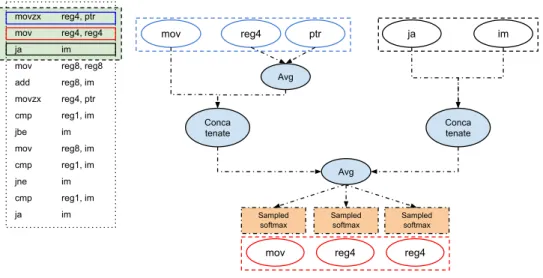
Our token embedding generation model shown in figure 4.3 is inspired by Asm2Vec which also uses instructions around a target token as context. Nonetheless, our model has a fundamentally different goal than Asm2Vec. DeepBinDiff learns token embeddings via program-wide random walks while Asm2Vec is trying to learn function and token em-beddings at the same time and only within the function. Therefore, we choose to modify Word2Vec CBOW model while Asm2Vec leverages the PV-DM model. We call it token2vec. Given a sequence of instructions in1, in2, ..., int. For an instruction ini which

contains an opcodepi and a set ofk(could be zero) operandsSetti, we model the instruction

embedding as concatenation of opcode embedding and the average of operand embeddings, as depicted in Equation 4.3 ini =embedpi|| 1 |Setti| ∗ k X n=1 embedtin (4.3)

Let tokeni be the set of tokens in a instruction ini, which contains the opcode pi

and operands set Setti. Then the objective of Token2Vec is to maximize the avcerage log

probability T(w) as given in Equation 4.4 and Equation 4.5

T(w) = 1 T T X t=1 X −c≤j≤c logp(tokent|int+j) (4.4) p(tokent|ink∈Ct) = exp(vT_in kvtokent) P ini∈Ctexp(v T inivtokent) (4.5)

To speed up the training step, according to [46, 41], we use the k negative sampling approach to approximate the log probability.

Feature Vector Generation

Once the token embeddings are generated, the last step is to generate feature vectors for basic blocks. Since each basic block could contain multiple instructions, each instruction in turn involves one opcode and potentially multiple operands, we calculate the average of the operand embeddings and then concatenate with the opcode embedding. We use Equasion 4.3 to calculate embeddings of each instruction. Therefore, for a block b = {in1, in2, .., inj} which contains j instructions, its feature vector F Vb is the merge of

its instruction embeddings. as depicted in Equation 4.6.

F Vb = I j i=1 (embedpi|| 1 |Setti| ∗ k X n=1 embedtin) (4.6) The symbol H

denotes the merge operation of instruction embeddings. We have multiple choice on this operation.Though concatenate is the best choice so that we can generate embeddings for basic blocks without losing any information from the instructions. The various length of basic blocks prevent us from doing so. As a result, we select some mathematical or statistical operations to convert all vectors into a single one.This operation will lose much information. However, those operations can handle instruction reorder which concatenate is not able to do. Here is some choices.

SUM Sum is the default choice of our approach. It is just sum all vectors up. This operation reserves most information and has the best performance in our evaluation.

movzx reg4, ptr mov reg4, reg4 ja im mov reg8, reg8 add reg8, im movzx reg4, ptr cmp reg1, im jbe im mov reg8, im cmp reg1, im jne im cmp reg1, im ja im mov reg4 ptr ja im Avg Conca tenate

mov reg4 reg4

Sampled softmax Sampled softmax Sampled softmax Conca tenate Avg

Figure 4.3: Token2Vec model used in DeepBinDiff

Statistical Operations We have MAX, MIN and MEAN for this category. We believe those operations is able to find out statistical features from instruction sequences.

PCA PCA(Principal components analysis) is also a statistical procedure introduced by Karl Pearson in 1901 [53], we split this method from the previous category is because it is widely used in current machine learning field and performs well on vector compression. However, from our evaluation, we found that the performance is still not as good as SUM.

RNN RNN is a good model to deal with sequential data. However, as a pre-processing step, RNN is too time consuming for this task, taking the number of basic blocks in real world programs into consideration.

4.3

Embedding Generation

Based on the ICFGs and feature vectors generated in prior steps, this component produces embeddings for basic blocks in the two input binaries with a goal that similar blocks can be associated with similar embeddings. Hence, block embeddings could be leveraged for binary diffing in later steps. To do so, DeepBinDiff first merges the two ICFGs into one graph and then perform matrix factorization based on Text-associated DeepWalk algorithm (TADW) [62] to generate block embeddings.

Since the most important building block for this component is the TADW algo-rithm, we first describe the algorithm in detail and present how basic block embeddings are generated. Then, we justify why graph merging is needed for TADW and report how DeepBinDiff accomplishes it.

4.3.1 TADW algorithm

Text-associated DeepWalk algorithm [62] is an automatic graph embedding learn-ing technique based on unsupervised deep learnlearn-ing. As suggested by name, it can be considered as an improvement over the DeepWalk algorithm [54].

DeepWalk DeepWalk algorithm is an online graph embedding learning algorithm that considers a set of short truncated random walks as a corpus in language modeling problem, and the graph vertices as its own vocabulary. The embeddings are then learned using ran-dom walks on the vertices in the graph. Accordingly, vertices that share similar neighbours will have similar embeddings.

E contains all the edges, the algorithm gets a shuffle ofV and generatesrandom walkswith a pre-defined lengthtfor each vertex in the shuffle and applies Skip-Gram model as defined previously in Equation 4.2 with respect to a fixed window size w. Just like Word2Vec, it also adopts the hierarchical Softmax to improve the efficiency.

Text-associated DeepWalk As described, DeepWalk excels at learning the structural information from a graph. Nevertheless, it does not consider the features from each vertex and differentiate them by their own uniqueness. As a result, Yang at el. [62] propose an improved algorithm called Text-associated DeepWalk (TADW) which is able to incorporate features of vertices into the network representation learning process. As mentioned before, to serialize ICFG and generate code sequences for word2vec, we have already performed random walk. Here we have to perform random walk again. However, this is not a redundant effort. It is proven that DeepWalk is equivalent to factorizing a matrixM ∈R|v|×|v| where each entry Mij is logarithm of the average probability that vertex vi randomly walks to

vertexvj in fixed steps. So we only performs a matrices factorization in this phase, instead

of a real random walk step. This discovery further leads to TADW algorithm depicted in Figure 4.4. It shows that it is possible to factorize the matrix M into the product of three matrices: W ∈Rk×|v|,H ∈Rk×f and a text featureT ∈Rf×|v|. Then,W is concatenated withHT to produce 2k-dimensional representations of vertices (embeddings).

4.3.2 Graph Merging

The goal for embedding generation of DeepBinDiff is to learn block embeddings such that similar blocks correspond to similar embeddings. To achieve this, DeepBinDiff

M

W

H

T

leverages TADW to generate embedding for each block. Since we have two ICFGs (one for each binary), the most intuitive way is to run TADW twice for the two graphs, hence, blocks that hold similar semantic (feature vectors) and structural information can obtain similar embeddings. However, this method has two drawbacks. First, it is inefficient to perform matrix factorization twice. Second, generating embeddings for the two graphs individually could in fact lower the effectiveness.

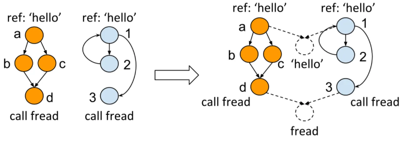
Take the example exhibited in Figure 4.5 for illustration. In this figure, we have two ICFGs and each graph has one block that calls a libc functionfread and another block that has a reference to string ‘hello’. Ideally, there is a great chance that these two pairs of nodes (‘a’ and ‘1’, ‘d’ and ‘3’) should matched. However, the feature vectors of these blocks may not be very similar as one block could contain multiple instructions and call or reference instruction is just one of them. Also, the two pairs also have quite different structural information. For example, node ‘a’ has two outgoing edges but no incoming edges while node ‘1’ has. As a result, it is possible that DeepBinDiff cannot generate very similar embeddings for the two pairs of nodes.

graph merging process to merge the two ICFGs before TADW. Particularly, it leverages Angr to extract the string references and detect calls to external libraries and system calls. Then, DeepBinDiff creates new virtual nodes for the strings and external library functions and draws edges from the callsites to these virtual nodes. This way, two graphs are merged into one graph on some terminal virtual nodes. By doing so, node ‘a’ and ‘1’ will have at least one common neighbor which boosts the similarity between them. Also, since we only merge the graphs on terminal nodes, the original structures of the two graphs are unchanged.

call fread

call fread

fread

call fread

call fread

ref: ‘hello’

ref: ‘hello’

ref: ‘hello’

ref: ‘hello’

‘hello’

a

b

c

d

3

2

1

a

b

c

d

1

2

3

Figure 4.5: Graph Merging

4.3.3 Basic Block Embeddings

With the merged graph, DeepBinDiff leverages TADW algorithm and performs matrix factorization to generate basic block embeddings.

More specifically, DeepBinDiff feeds the merged graph from two ICFGs and the block feature vectors into TADW for multiple iterations of optimization. The algorithm factorizes the matrix M into three matrices by minimizing the loss function depicted in

Equation 4.7 using Alternating Least Squares (ALS) algorithm [38]. It stops when the loss converges or after a fixedn iterations.

min W,H||M−W T_HT||2 F + λ 2(||W|| 2 F +||H||2F) (4.7)

On that account, each generated basic block embedding contains not only the information about the block itself, but also the information from the ICFG structural in-formation. The generated embeddings are essential for binary diffing.

4.4

Code Diffing

Once the basic block embeddings are generated, the last step in DeepBinDiff is to perform code diffing. The goal is to find the optimal matching between blocks that maximizes the similarity for the two input binaries.

One spontaneous choice for this task is to consider blocks from one binary as workers, blocks from the other binary as jobs and embedding similarities as weights, then perform linear assignment to come up with the global optimal matching. This method, however, suffers from two major limitations. First, binaries could contain thousands of blocks or even more and linear assignment at this scale is inefficient. Second, although embeddings do include structural information, linear assignment itself does not consider any graph information. Thus, it is still likely to make mistakes when matching very similar blocks.

Another possible way to improve the performance is to conduct two-level linear assignment at function level and block level. Instead of matching blocks directly, we match

functions in the two binaries first by using function level embeddings. Then, blocks within the matched function pairs can be further matched with block embeddings. This approach can be thwarted by compiler optimizations that alter the function boundary such as function inlining.

Algorithm 1 K-Hop Greedy Matching Algorithm

1: Setinitial ← {initial match from virtual nodes}

2: Setmatched←Setinitial

3: SetcurrP airs←Setinitial

4:

5: whileSetcurrP airs != empty do

6: (node1, node2)←SetcurrP airs.pop()

7: nbnode1 ← GetKHopNeighbors(node1) 8: nbnode2 ← GetKHopNeighbors(node2)

9: newP air← FindMaxUnmatched(nbnode1,nbnode2) 10: if newP air != NULLthen

11: Setmatched ←Setmatched∪newP air

12: SetcurrP airs ←SetcurrP airs∪newP air

13: end if

14: end while

15: Setunreached ← {blocks that are not yet matched}

16: Setmatched←Setmatched∪ LinearAssign(Setunreached)

4.4.1 K-Hop Greedy Matching

To tackle this problem, we introduce a K-hop greedy matching algorithm. The high-level idea is to benefit from the ICFG structural information and find matching blocks based on the similarity calculated from block embeddings within the neighbors of already matched ones.

As presented in Algorithm 1, it extracts initial matchingSetinitialfrom the inserted

virtual nodes during graph merging described in Section 4.3.2 and producesSetmatchedas the

binary diffing result. The initial matched pairs are generated by using the string references and calls to external functions. For example, if each binary only has one block that refers to string “hello world”, it is highly likely that these two blocks will match. Starting from the initial set, the algorithm loops and explores the neighbors of the already matched pairs in GetKHopN eighbors() in Ln.7-8. DeepBinDiff then sorts the similarities between neighbor blocks and picks the pair bearing highest similarity by calling F indM axU nmatched() in Ln.9. During this step, the algorithm empirically sets a threshold of 0.25 to make sure the new matching blocks are similar enough. This process is repeated until all K-neighbors of matched pairs are explored and matched. Note that after the loop, there may still exist unmatched blocks due to unreached code (dead code) or low similarity within K-hop neighbors. The algorithm then performs linear assignment and finds the optimal matching among them in Ln.16. Finally, the algorithm returnsSetmatched as the binary diffing result.

Chapter 5

Evaluation

In this section, we evaluate DeepBinDiff with respect to its effectiveness and effi-ciency for two different binary diffing scenarios: cross-version diffing and cross-optimization level diffing. To our best knowledge, this is the first research work that comprehensively examines the effectiveness of binary diffing tools under the cross-version setting.

Furthermore, we conduct a case study to demonstrate the usefulness of DeepBin-Diff in real-world vulnerability analysis.

5.1

Experimental Setup

Our experiments are performed on a moderate desktop computer running Ubuntu 18.04LTS operating system with Intel Core i7 CPU, 16GB memory and no GPU. The feature vector generation and block embedding generation components in DeepBinDiff are expected to be significantly accelerated if GPUs are utilized since the two components are built upon deep learning models.

5.2

Implementation

In this section, we are going to introduce the implementation of our prototype, DeepBinDiff. The whole system consists of about 2500 lines of python code. Our system is built on the top of Angr [1] and Tensorflow [10]. We uses Angr to disassemble binaries and recover ICFGs, while we uses Tensorflow to implement our own word2vec model and TADW model. Here is some details.

Pre-Processing In pre-processing phase we use Angr to disassemble binaries and recover ICFGs. To generate feature vectors, we use Tensorflow to implement our own modified Token2Vec model. Table 5.1 shows some hyper-parameters for this step. We provide two different loss functions. The first is sampled softmax loss, the second is NCE loss which is also called noise-contrastive estimation loss. They are both sampling approaches mentioned in section 4.2.2. NCE loss tries to simplify the problem to a bi-type classification problem, which can be solved by logistic regression. Sampled softmax loss tries to randomly pick a few samples to approximate the softmax probability. Those two loss function is widely used in classification problems and has been implemented by Tensorflow.

For feature vector generation of basic blocks we also leave multiple choices. We have sum, mean, min and max function to merge embeddings of instructions. According to our observation, the summary function performs best in most cases over previous choices, so we leave sum as default.

Embedding Generation As introduced in section 4.3.1, we use TADW to collect struc-tural information. Our implementation is based on a python library called OpenNE [7].

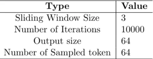
Table 5.1: Hyper Parameter selection

Type Value

Sliding Window Size 3 Number of Iterations 10000

Output size 64 Number of Sampled token 64

Considered that structural information has been collected and inserted into the embed-dings in this step, we adjust our embedding size to 128. A decaying learning rate, which is called lambda in TADW [62] is configured to 0.1.

5.3

Datasets & Baseline Techniques

5.3.1 Datasets.

To thoroughly evaluate the effectiveness of DeepBinDiff, we collect a number of representative datasets. More specifically, we utilize three binary sets - Coreutils [3], Diffu-tils [4] and FinduDiffu-tils [5] with a total of 113 binaries for the evaluation of effectiveness and efficiency. Multiple different versions of the binaries (5 versions for Coreutils, 4 versions for Diffutils and 3 versions of Findutils) are collected with wide time spans between the oldest and newest versions (13, 15, 7 years respectively). This setting ensures that each collected version has enough distinctions such that binary diffing results among them are meaningful and representative.

We then compile the programs using GCC 5.4 with 3 different compiler opti-mization levels (O1, O2 and O3) to produce binaries equipped with different optiopti-mization techniques. This dataset is leveraged to show the effectiveness of DeepBinDiff in terms of

cross-optimization level diffing.

Moreover, we leverage a popular general-purpose cryptography library OpenSSL [8] for vulnerability analysis case study. In the case study, we use two different real-world vul-nerabilities to demonstrate the advantage of DeepBinDiff in practice.

5.3.2 Baseline Techniques.

With the aforementioned datasets, we run DeepBinDiff and compare it against another two state-of-the-art baseline techniques (Asm2Vec [25] and BinDiff [9]). Note that Asm2Vec is designed only for function level similarity detection. We leverage its algorithm to generate token embeddings and take the same procedure in the paper to average operand embeddings and concatenate with opcode embedding to generate instruction embeddings. Then, we further sum them up to produce block embeddings and perform binary diffing with the same K-hop greedy matching algorithm adopted by DeepBinDiff.

5.4

Ground Truth Collection

Ground truth information about how blocks from two binaries should be matched is required when measuring the effectiveness of DeepBinDiff. To this end, we rely on source code matching and debug symbol information to collect ground truth information.

Particularly, for two input binaries to be diff’ed, we first extract source file names from the binaries and then use Myers algorithm [50] to perform text based matching for the source code of the two binaries in order to get the line number matching. We take two steps to ensure the soundness of our extracted ground truth information. First, we only collect

identical lines of source code as matching but ignore the modified ones. Second, our ground truth collection process is being deliberately conservative to remove the matching lines like macros which could expand to multiple lines of code. Therefore, although our source code matching is by no means complete, it is guaranteed to contain zero false positive.

Once we have the line number mapping between the two binaries, readelf tool is used to extract debug information to understand the mapping between line numbers and program addresses. Eventually, the ground truth is collected by examining the blocks of the two binaries containing program addresses that map to the matched line numbers. This way, we can successfully collect ground truth block matching information for every pair of binaries.

Example. Take the diffing between v5.93 and v8.30 of Coreutils binarychown for illus-tration. To collect ground truth information for block matching between the two binaries, we first extract source file names from them and perform text-based matching between the corresponding source files. By matching the source files chown.c in the two versions, we know Ln. 288 in v5.93 should be matched to Ln. 273 in v8.30. Together with the debug information extracted byreadelf, a matching between address 0x401cf8 in v5.93chown and address 0x4023fc in v5.93chown can be established.

Finally, we use Angr to generate basic blocks for the two binaries. By checking the addresses within the blocks, we know block 3 in v5.93 chown should be matched to block 13 in v8.30chown. Therefore, we collect the ground truth information about how the blocks between the two binaries should be matched and we further use this information to

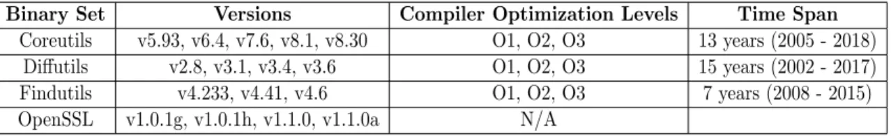
Table 5.2: Experimental Datasets

Binary Set Versions Compiler Optimization Levels Time Span

Coreutils v5.93, v6.4, v7.6, v8.1, v8.30 O1, O2, O3 13 years (2005 - 2018)

Diffutils v2.8, v3.1, v3.4, v3.6 O1, O2, O3 15 years (2002 - 2017)

Findutils v4.233, v4.41, v4.6 O1, O2, O3 7 years (2008 - 2015)

OpenSSL v1.0.1g, v1.0.1h, v1.1.0, v1.1.0a N/A

measure the correctness of the diffing results produced by DeepBinDiff.

5.5

Effectiveness

With the experimental datasets and ground truth information collected, we evalu-ate the effectiveness of DeepBinDiff by performing diffing between binaries across different versions and optimization levels, and checking the results against the ground truth infor-mation. We also compare the results against two state-of-the-art baseline techniques.

5.5.1 Evaluation Metrics

In the evaluation, we use precision and recall metrics to measure the effectiveness of the diffing results produced by diffing tools. The matching result M from DeepBinDiff for two given binaries can be presented as a set of block matching pairs with a length of x. Similarly, the ground truth information G for the two binaries can be presented as a set of block matching pairs with a length of y. We present them in Equation 5.1 and 5.2. Elements in set M and G show matching relationship between two basic blocks from the two binaries in the matching result from DeepBinDiff and ground truth information respectively.

M ={(m1, m 0 1),(m2, m 0 2), ...,(mx, m 0 x)} (5.1) G={(g1, g 0 1),(g2, g 0 2), ...,(gy, g 0 y)} (5.2)

We then define two subsets ofM: McandMu, representing correct matching and

unknown matching respectively. Correct matchMc=M∩Gis the intersection of our result

M and ground truthGwhich gives us the correct block matching pairs. Unknown matching resultMurepresents the block matching pairs that no block in these pairs is ever appeared in

ground truth. Thus, we have no idea whether these matching pairs are correct. This could happen due to the conservativeness of our ground truth collection process. Consequently, M−Mu−Mc portrays the matching pairs in M that are not in Mcnor in Mu, therefore,

all pairs inM−Mu−Mc are confirmed to be incorrect matching pairs.

Once we have M andGformally presented, we use precision and recall metrics to show the quality of diffing results. The precision metric presented in Equation 5.3 gives us the percentage of correct matching pairs among all the known pairs (correct and incorrect).

P recision= ||M∩G||

||M∩G||+||M −Mu−Mc||

(5.3)

The recall metric shown in Equation 5.4 is produced by finding the intersection of setsM and G and dividing its size by the size of setG. This metric shows the percentage of ground truth pairs that are correctly matched by the diffing tool.

Recall= ||M∩G||

5.5.2 Cross-version Diffing

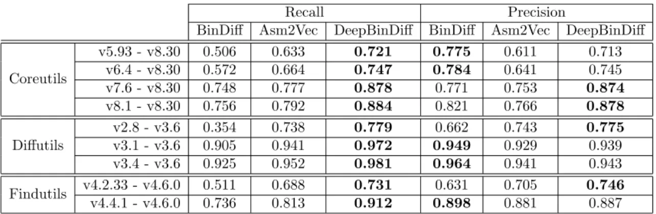
In this experiment, we benchmark the performance of DeepBinDiff, BinDiff and Asm2Vec by conducting binary diffing between different versions of binaries (all compiled with O1 compiler optimization level) in Coreutils, Diffutils and Findutils. We report the average recall and precision for each tool under different experimental settings in Table 5.3. As we can see, DeepBinDiff outperforms Asm2Vec and BinDiff across all versions of the three datasets in terms of recall, especially when the two diffed versions have a large gap. For example, for Coretuils diffing between v5.93 and v8.30, DeepBinDiff improves the recall by 14% and 42% over Asm2Vec and BinDiff. Also, we can observe that Asm2Vec which carries the semantic information for tokens, in general has better recall than the de-facto commercial tool BinDiff. This evaluation results show that including semantic information during analysis can improve the effectiveness of diffing. Moreover, since a major difference between DeepBinDiff and Asm2Vec is the structural information generated from TADW, we can also draw the conclusion that structural information can help boost the quality of diffing results by a large margin.

Interestingly, we also notice that BinDiff sometimes can produce higher precision than Asm2Vec and DeepBinDiff. We investigate the detailed results and see that BinDiff has a very conservative matching strategy. It usually only matches the basic blocks with very high similarity score and leaves the other blocks unmatched. Therefore, BinDiff generates much short matching list than DeepBinDiff which uses K-hop greedy matching to maximize the matching.

Table 5.3: Cross-version Binary Diffing Results

Recall Precision

BinDiff Asm2Vec DeepBinDiff BinDiff Asm2Vec DeepBinDiff

Coreutils v5.93 - v8.30 0.506 0.633 0.721 0.775 0.611 0.713 v6.4 - v8.30 0.572 0.664 0.747 0.784 0.641 0.745 v7.6 - v8.30 0.748 0.777 0.878 0.771 0.753 0.874 v8.1 - v8.30 0.756 0.792 0.884 0.821 0.766 0.878 Diffutils v2.8 - v3.6 0.354 0.738 0.779 0.662 0.743 0.775 v3.1 - v3.6 0.905 0.941 0.972 0.949 0.929 0.939 v3.4 - v3.6 0.925 0.952 0.981 0.964 0.941 0.943 Findutils v4.2.33 - v4.6.0 0.511 0.688 0.731 0.631 0.705 0.746 v4.4.1 - v4.6.0 0.736 0.813 0.912 0.898 0.881 0.887

Table 5.4: Cross-optimization level Binary Diffing Results

Recall Precision

BinDiff Asm2Vec DeepBinDiff BinDiff Asm2Vec DeepBinDiff

Coreutils v5.93 O1 - O3 0.571 0.556 0.652 0.638 0.537 0.668 v5.93 O2 - O3 0.837 0.905 0.976 0.944 0.855 0.932 v6.4 O1 - O3 0.576 0.589 0.676 0.646 0.569 0.697 v6.4 O2 - O3 0.838 0.899 0.978 0.954 0.848 0.939 v7.6 O1 - O3 0.484 0.627 0.668 0.674 0.602 0.704 v7.6 O2 - O3 0.840 0.898 0.953 0.944 0.845 0.913 v8.1 O1 - O3 0.480 0.628 0.673 0.677 0.601 0.713 v8.1 O2 - O3 0.835 0.868 0.921 0.942 0.839 0.901 v8.30 O1 - O3 0.508 0.516 0.607 0.620 0.495 0.638 v8.30 O2 - O3 0.842 0.884 0.952 0.954 0.832 0.903 Diffutils v2.8 O1 - O3 0.467 0.779 0.831 0.613 0.755 0.828 v2.8 O2 - O3 0.863 0.955 0.979 0.953 0.936 0.966 v3.1 O1 - O3 0.633 0.801 0.816 0.655 0.647 0.775 v3.1 O2 - O3 0.898 0.902 0.943 0.966 0.925 0.964 v3.4 O1 - O3 0.577 0.712 0.754 0.708 0.698 0.715 v3.4 O2 - O3 0.903 0.911 0.935 0.953 0.943 0.967 v3.6 O1 - O3 0.735 0.876 0.865 0.715 0.811 0.853 v3.6 O2 - O3 0.919 0.954 0.962 0.966 0.922 0.952 Findutils v4.233 O1 - O3 0.633 0.695 0.783 0.768 0.637 0.799 v4.233 O2 - O3 0.933 0.952 0.983 0.968 0.931 0.981 v4.41 O1 - O3 0.677 0.715 0.821 0.731 0.677 0.882 v4.41 O2 - O3 0.839 0.912 0.951 0.964 0.952 0.967 v4.6 O1 - O3 0.563 0.636 0.763 0.633 0.721 0.791 v4.6 O2 - O3 0.958 0.935 0.961 0.932 0.915 0.954

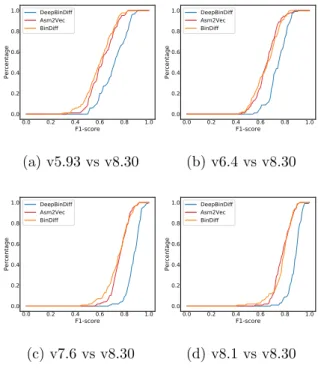
We further present the Cumulative Distribution Function (CDF) figures for F1-scores of the three diffing techniques on Coreutils binaries in Figure .1. Again, from the CDF figures we can see that Asm2Vec and BinDiff have similar F1-scores while DeepBinDiff performs much better. And due to the high precision, BinDiff can even have higher F1-scores than Asm2Vec. In a nutshell, DeepBinDiff can exceed two baseline techniques by large margins with respect to cross-version binary diffing.

5.5.3 Cross-optimization level Diffing

We then conduct experiments to measure the effectiveness of the three techniques in terms of cross-optimization level binary diffing. We perform diffing between the binaries with the same version but under different optimization levels. Particularly, each binary is diffed twice (O1 versus O3 and O2 versus O3). We report the average recall and precision for all settings in Table 5.4.

As shown, just like cross-version binary diffing, DeepBinDiff could outperform Asm2Vec and BinDiff for most of the settings in recall rate. The only exception is the Diffutils v3.6 O1 to O3 diffing where Asm2Vec has a recall rate of 0.876 while DeepBinDiff obtains 0.865. It is because there are only 4 binaries in Difftuils and most of them are small. In this special case, program-wide structure information may become less useful. Still, DeepBinDiff could defeat Asm2Vec for all other settings, even for Diffutils. Also, BinDiff still enjoys a high precision rate, sometimes higher than DeepBinDiff.

One thing we can see from the results is that cross-optimization level binary diffing is more difficult than cross-version diffing since the recall and precision rates are lower. This is because of the compiler optimization techniques could greatly transform the binaries.

However, we anticipate DeepBinDiff and Asm2Vec to achieve better results if trained with more samples.

5.6

Efficiency

We then conduct experiments to show the efficiency of our system. The run-ning time of DeepBinDiff can be split into four parts: trairun-ning time, pre-processing time, embedding generation time and matching time.

Training Time We train our token embedding generation model with the binaries in our dataset. Random walks are generated for each binary to produce one article for training our model. We stop the training for each binary when loss converges or it hits 10000 steps. In total, It takes about 30 hours for our machine to finish the whole training process. We could retrain our model when new binaries are fed into DeepBinDiff. For comparison, Asm2Vec also needs this training time to generate its model while BinDiff does not need any training time. Note that training the model is only an one-time effort and the training process could be significantly accelerated if GPUs are used.

Pre-processing Time DeepBinDiff relies on Angr for ICFG generation. It takes only an average of 12.264s DeepBinDiff to finish the graph generation on one binary. Then, our system applies the pre-trained model to generate token embeddings and calculates the feature vectors for each basic block. Applying the model and calculating the feature vector only takes less than 100ms for one binary. BinDiff which uses IDA pro for pre-processing takes similar time for its pre-processing.

Embedding Generation The most heavy part of DeepBinDiff is the embedding gener-ation which utilizes TADW to factorize a matrix. On average, it takes 591s on average to finish embedding generation for one binary. One way to accelerate the process is to use a more efficient algorithms other than the Alternating Least Squares (ALS) algorithm for TADW matrix factorization. For example, CCD++ [63] is demonstrated to be 40 times faster than ALS algorithm.

Matching Time K-hop greedy matching algorithm is efficient in that it limits the search space by searching only within the K-hop neighbors for the two matched blocks. On average, it takes DeepBinDiff 45 seconds to finish the matching. BinDiff, for comparison, takes only 3.4s to finish matching since it uses many heuristics to avoid graph matching.

5.7

Case Study

Besides the above experiments, we also evaluate DeepBinDiff with real-world vul-nerability analysis to showcase its efficacy in practice. Two representative vulnerabilities in OpenSSL [8] are utilized for an in-depth comparison among our tool and the state-of-the-art commercial diffing tool BinDiff.

5.7.1 DTLS Recursion Flaw

The first vulnerability (CVE-2014-0221) happens in OpenSSL v1.0.1g and before, gets fixed in v1.0.1h. It is a Datagram Transport Layer Security (DTLS) recursion flaw vulnerability which allows attackers to send an invalid DTLS handshake to OpenSSL client to cause recursion and eventually crash.

Listing 5.1 shows the vulnerability along with the patched code. As listed, patching is made to avoid the recursive call by changing it to agoto statement (Ln. 10-11).

Listing 5.1: DTLS Recursion Flaw

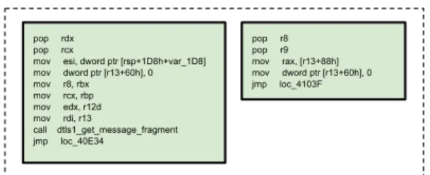
1 s t a t i c l o n g d t l s 1 _ g e t _ m e s s a g e _ f r a g m e n t () { 2 int i , al ; 3 ... 4 + redo: ; 5 if(( f r a g _ l e n = f r a g m e n t ( s , max , ok )) { 6 ... 7 if ( s - > m s g _ c a l l b a c k ) { 8 s - > m s g _ c a l l b a c k (0 , s - > v e r s i o n ) 9 - return dtls1 get message fragment(); ;

10 + goto redo;

11 }

To analyze this vulnerability, we feed a vulnerable version as well as a patched version of OpenSSL into the diffing tools and see if the tools can generate correct matching between the blocks that contain the vulnerability and the patch.

Partial results from BinDiff and DeepBinDiff are shown in Figure 5.1. This match-ing is hard because in v1.0.1h, the patched functiondts1 get message f ragment() is inlined into another function nameddts1 get message(). BinDiff matches the vulnerable function in v1.0.1h with its caller in v1.0.1g, leaving the originaldts1 get message() in v1.0.1g un-matched.