Peter Haan
Arne Uhlendorff
Estimation of Multinomial Logit Models with
Unobserved Heterogeneity Using Maximum
Simulated Likelihood
Opinions expressed in this paper are those of the author and do not necessarily reflect views of the Institute.
IMPRESSUM © DIW Berlin, 2006 DIW Berlin
German Institute for Economic Research Königin-Luise-Str. 5
14195 Berlin
Tel. +49 (30) 897 89-0 Fax +49 (30) 897 89-200
www.diw.de
ISSN print edition 1433-0210 ISSN electronic edition 1619-4535
All rights reserved.
Reproduction and distribution in any form, also in parts, requires the express written permission of DIW Berlin.
Estimation of multinomial logit models with unobserved
heterogeneity using maximum simulated likelihood
Peter Haan∗ and Arne Uhlendorff†
March 29, 2006
Abstract
In this paper we suggest a Stata routine for multinomial logit models with unob-served heterogeneity using maximum simulated likelihood based on Halton sequences. The purpose of this paper is twofold: First, we provide a description of the techni-cal implementation of the estimation routine and discuss its properties. Further, we compare our estimation routine to the Stata programgllammwhich solves integration using Gauss Hermite quadrature or Bayesian adaptive quadrature. For the analysis we draw on multilevel data about schooling. Our empirical findings show that the esti-mation techniques lead to approximately the same estiesti-mation results. The advantage of simulation over Gauss Hermite quadrature is a marked reduction in computational time for integrals with higher dimensions. Bayesian quadrature, however, leads to very stable results with only a few quadrature points, thus the computational advantage of Halton based simulation vanishes in our example with one and two dimensional integrals.
Keywords: multinomial logit model, panel data, unobserved heterogeneity, maximum simulated likelihood, Halton sequences
∗DIW Berlin, FU Berlin. Correspondence: Peter Haan, DIW Berlin, K¨onigin-Luise-Straße 5, 14195
Berlin, e-mail: [email protected]
†DIW Berlin, IZA Bonn. Correspondence: Arne Uhlendorff, DIW Berlin, K¨onigin-Luise-Straße 5, 14195
1
Introduction
In many empirical applications, e.g. estimation of mixed logit models, the researcher is faced with the problem that standard maximum likelihood estimation can not be ap-plied as analytical integration is not possible. Instead, methods such as quadrature or simulation are required for approximation of the integral. In this paper we suggest a Stata routine for multinomial logit models with unobserved heterogeneity using maximum simulated likelihood (MSL).1 The purpose of this paper is twofold. First, we provide
a description of the technical implementation of the estimation routine and discuss its properties. Further, we compare our estimation routine with the program gllammwhich is implemented in Stata. gllamm is a very flexible programm incorporating a variety of multilevel models including mixed logit, see Rabe-Hesketh, Skrondal, and Pickles (2004) or Skrondal and Rabe-Hesketh (2005). Our routine differs fromgllammfor computational reasons: whereas ingllammintegrals are solved using classical Gauss Hermite or Bayesian adaptive quadrature, we suggest simulation based on Halton sequences for integration. In our analysis we compare the performance of the estimation techniques using multilevel data about schooling from thegllammmanual.
Our empirical findings show that when the integral is reasonably well approximated the estimation techniques lead to nearly the same results. The advantage of Halton based simulation over classical Gauss Hermite quadrature is computational time; this advantage is increasing with the dimensions of the integral. Bayesian quadrature, however, leads to very stable results with only a few quadrature points, thus the computational advantage of Halton based simulation vanishes in our example with one and two dimensional integrals.
2
Multinomial logit models with unobserved heterogeneity
Mixed logit models are a highly flexible class of models approximating any random utility model (Train, 2003). In our application we focus on a specific model of this broad class, the multinomial logit panel data model with random intercepts.2 However, the results we
present can be extended to other mixed logit models both with panel and cross sectional data.
We assume that individual i is faced with J different choices at time t. As well documented in the literature, see e.g. Train (2003), the probability of making choice j
conditional on observed characteristics Xit that vary between individuals and over time
and unobserved individual effectsαi that are time constant can be expressed as follows:
1Our approach closely follows Train (2003). Train implemented a program for mixed logit models in
GAUSS.
P(j|Xit, αi) = exp(Xitβj+αij)
Σjk=1exp(Xitβk+αik)
. (1)
As the choice probabilities are conditioned on αi it is necessary to integrate over
the distribution of the unobserved heterogeneity. Thus, the sample likelihood for the multinomial logit with random intercepts has the following form:
L= N Y i=1 Z ∞ −∞ T Y t=1 J Y j=1 Ã exp(Xitβj+αj) Σjk=1exp(Xitβk+αk) !dijt f(α)dα, (2)
where dijt=1 if individual i chooses alternative j at time t and zero otherwise. The
coefficient vector and the unobserved heterogeneity term of one category are set to 0 for identification of the model. For convenience we assume throughout our analysis that the unobserved heterogeneity α follows a multivariate normal distribution with mean a and variance-covariance matrix W, α ∼ f(a, W). In most applications α is specified to be normally distributed, however as Train (2003) points out the distributional assumption depends on the research question; if more appropriate, distributions such as log-normal or uniform can be assumed.
In order to maximize the sample likelihood it is necessary to integrate over the dis-tribution of unobserved heterogeneity. Yet, there exists no analytical solution for the integral in equation (2). In the literature numerous methods for integral approximation have been suggested and discussed. We focus on classical Gauss Hermite quadrature, Bayesian adaptive quadrature and simulation based on Halton sequences.
Gauss Hermite and adaptive quadrature
Gauss Hermite and adaptive quadrature is discussed in detail in Rabe-Hesketh, Skrondal, and Pickles (2002). The idea behind the Gauss Hermite quadrature is to approximate an integral by a specified number of discrete points. Adaptive quadrature is a Bayesian method that extends Gauss Hermite quadrature by making use of the posterior distribution of the unobserved heterogeneity. This extremely increases the accuracy of integration. The Stata programgllammincorporates both integration methods, yet adaptive quadrature is highly recommended for its higher accuracy (Rabe-Hesketh, Skrondal, and Pickles, 2002).
Estimation with Maximum Simulated Likelihood
We suggest to integrate over the unobserved heterogeneity by using simulation and to maximize a simulated likelihood . The intuition behind MSL is to draw R values from the distribution of the unobserved heterogeneity with variance-covariance matrixW. For
each of these draws the likelihood is calculated and then averaged over theR draws. That implies, instead of the exact likelihood a simulated sample likelihood (SL) is maximized:
SL= N Y n=1 1 R R X r=1 T Y t=1 J Y j=1 Ã exp(Xitβj+αrj) Σjk=1exp(Xitβk+αr k) !dijt . (3)
Consider an example with three different choices (j= 3). For identificationβ1 andαi1
are normalized to zero. We assume that the unobserved heterogeneity differs between the two other choices (αi2 6=αi3) and allow for correlation of these terms. Hence, the
distrib-ution of the unobserved heterogeneity can be described by a bivariate normal distribdistrib-ution with: α∼f a2 a3 , var2 cov23 cov23 var3 . (4)
That implies when applying MSL we need to approximate a two dimensional integral. Each draw r consists of two values (²2, ²3)0 which follow a standard normal distribution.
We apply a Cholesky decomposition of the variance-covariance matrix W. A Cholesky factorL of matrixW is defined such thatLL’ =W. Then, the unobserved effects αr are
calculated byαr=L²r. For our example that implies:
α2 α3 = l11 0 l21 l22 ²2 ²3 . (5)
The example can be easily extended to more complex choice situations. However, with increasing number of choices integration becomes more and more time intensive as the dimension of the integral increases.
Instead of using random draws to obtain (²2, ²3)0we follow Train (2003) and recommend
to base simulation on Halton sequences. Halton sequences generate quasi random draws that provide a more systematic coverage of the domain of integration than independent random draws and induce a negative correlation over observations. Several studies such as Train (1999) and Bhat (2001) have shown that in the context of mixed logit models the accuracy can be markedly increased by making use of Halton sequences; the authors find in their studies that the results are more precise with 100 Halton draws than with 1000 random draws. These results confirm that quasi-random sequences go along with a lower integration error and faster convergence rates and therefore require clearly less number of draws compared to pseudo-random sequences.3 However, as Train (2003) points out
3The expected integration error using pseudo-random sequences is of orderR−.5 while the theoretical
upper bound for the integration error using quasi-random sequences is of orderR−1, see Bhat (2001) or
the use of Halton draws in simulation based estimation is not completely understood and caution is required. He provides an example of Halton sequences and discusses advantages and anomalies of this method in the context of mixed logit models. The advantages of Halton draws might not hold for other models in the same way, see for example Cappellari and Jenkins (2006) who discuss Halton sequences for multivariate probit models.
3
Stata Routine for MSL estimation
In this section we provide aml modelstatement which refers to a multinomial logit panel data model with two potentially correlated random intercepts that follow a bivariate nor-mal distribution. This example can easily be extended to models with a higher number of alternatives.
For illustration, we apply our program to a real data set about teachers’ evaluation of pupils behaviour.4 Teachers group pupils in three different quality levels (tby). The data
provide information about 3939 pupils in 48 schools. The panel dimension of the data is not over time but over a certain school (scy3), hence in the estimation we can control for unobserved school specific effects. For simplicity we condition the rating of teachers next to unobservable effects only on one observable variable, namely sex.
Before executing our program for MSL estimation we apply the program mdraws by Cappellari and Jenkins (2006) to generate Halton Sequences and calculate the correspond-ing values followcorrespond-ing a standard normal distribution. Alternatively,mdrawscan be used to create pseudo-normal draws.
It is important that, for each draw, the values (random 1‘r’ and random 2‘r’) are the same for one observation within each unit, here within each school. Therefore, we create draws for every school and merge these draws to every pupil within each school. In this example we approximate the integral using 50 draws from the Halton sequence. We specify the primes used to create the Halton sequences as 7 and 11, because we later on estimate models with 150 draws and the number of draws should not be an integer multiple of any of the used primes, see e.g. Cappellari and Jenkins (2006) for details. Interesting to note is that computational time and estimation results slightly vary with the chosen primes. This fact is documented by Train (2003) who found that the choice of the primes might noticeably affect the estimated coefficients.
. matrix p = (7, 11) . global draws "50" . use "jspmix.dta",clear . keep scy3
. sort scy3
leads to the same improvement of accuracy as a hundred fold increase in the number of pseudo-random draws.
4The data set is available as an ASCII file jspmix.dat (http://www.gllamm.org/jspmix.dat).
. by scy3: keep if _n==1 (1265 observations deleted) . mdraws, neq(2) dr($draws) prefix(c) burn(10) prime (p)
Created 50 Halton draws per equation for 2 equations. Number of initial draws dropped per equation = 10 . Primes used:
7 11
. local repl=${draws} . local r=1
. while ‘r’ <= ‘repl’ {
2. by scy3: gen random_1‘r’=invnorm(c1‘r’) 3. by scy3: gen random_2‘r’=invnorm(c2‘r’) 4. local r=‘r’+1
5. } . sort scy3
. save mdraws_${draws}, replace file mdraws_50.dta saved . use "jspmix.dta",clear
. sort scy3
. merge scy3 using mdraws_${draws}.dta . drop _merge
. sort scy3
To get appropriate starting values for the coefficient vector, we usemlogitto estimate a multinomial logit model without random intercepts. The variables a1, a2, and a3 take on the value one if the choice 1, 2 or 3 is made, respectively, otherwise zero.
. mlogit tby sex, base(1) (output deleted)
. matrix Init= e(b) . gen a1=0
. gen a2=0 . gen a3=0
. replace a1=1 if tby==1 (329 real changes made) . replace a2=1 if tby==2 (678 real changes made) . replace a3=1 if tby==3 (306 real changes made) . sort scy3
The following ml model statement can be applied independently of the chosen type of draws (e.g. pseudo-random or Halton draws). We apply the method d0 because we esti-mate panel data models with joint unobserved heterogeneity for groups of observations.5
program define mlogit_sim_d0 args todo b lnf
tempvar etha2 etha3 random1 random2 lj pi1 pi2 pi3 sum lnpi L1 L2 last tempname lnsig1 lnsig2 atrho12 sigma1 sigma2 cov12
mleval ‘etha2’ = ‘b’, eq(1) mleval ‘etha3’ = ‘b’, eq(2)
mleval ‘lnsig1’ = ‘b’, eq(3) scalar mleval ‘lnsig2’ = ‘b’, eq(4) scalar mleval ‘atrho12’ = ‘b’, eq(5) scalar
5The principles of computing maximum likelihood estimators with Stata are described in Gould,
qui {
scalar ‘sigma1’=(exp(‘lnsig1’))^2 scalar ‘sigma2’=(exp(‘lnsig2’))^2
scalar ‘cov12’=[exp(2*‘atrho12’)-1]/[exp(2*‘atrho12’)+1]*(exp(‘lnsig2’))*(exp(‘lnsig1’)) gen double ‘random1’ = 0
gen double ‘random2’ = 0 gen double ‘lnpi’=0 gen double ‘sum’=0 gen double ‘L1’=0 gen double ‘L2’=0
by scy3: gen byte ‘last’=(_n==_N) gen double ‘pi1’= 0
gen double ‘pi2’= 0 gen double ‘pi3’= 0 }
matrix W = ( ‘sigma1’ , ‘cov12’ \ ‘cov12’ , ‘sigma2’) capture matrix L=cholesky(W)
if _rc != 0 {
di "Warning: cannot do Cholesky factorization of rho matrix" }
local l11=L[1,1] local l21=L[2,1] local l22=L[2,2]
local repl=${draws} local r=1 while ‘r’ <= ‘repl’ { qui {
replace ‘random1’ = random_1‘r’*‘l11’
replace ‘random2’ = random_2‘r’*‘l22’ + random_1‘r’*‘l21’
replace ‘pi1’= 1/(1 + exp(‘etha2’+‘random1’)+exp(‘etha3’+‘random2’)) replace ‘pi2’= exp(‘etha2’+‘random1’)*‘pi1’
replace ‘pi3’= exp(‘etha3’+‘random2’)*‘pi1’ replace ‘lnpi’=ln(‘pi1’*a1+‘pi2’*a2+‘pi3’*a3) by scy3: replace ‘sum’=sum(‘lnpi’)
by scy3: replace ‘L1’ =exp(‘sum’[_N]) if _n==_N by scy3: replace ‘L2’=‘L2’+‘L1’ if _n==_N }
local r=‘r’+1 }
qui gen ‘lj’=cond(!‘last’,0, ln(‘L2’/‘repl’)) qui mlsum ‘lnf’=‘lj’
if (‘todo’==0|‘lnf’>=.) exit end
Instead of estimating the variances and the correlation coefficient directly we estimate transformed variables of these parameters, i.e. the logarithm of the standard deviations (lnsig1 and lnsig2) and the inverse hyperbolic tangent of ρ (atrho12), to constrain them
within their valid limits. Therefore, the first step in our program is to calculate the vari-ances (sigma1 and sigma2) and the covariance (cov12) of the bivariate normal distribution. After that we apply a Cholesky decomposition of the covariance matrixW. In order to do this, the matrixW has to be positive definite. If this is not the case, our program traps the error, shows a warning and uses the most recent estimate of W. This is assured by the commandcapture.6
Within the following loop we calculate the likelihood for each draw based on the individual specific quasi-random terms random1 and random2. The two terms random1 ‘r’ and random2 ‘r’ are multiplied with the elements of the Cholesky matrix L, following equation (5). The probabilities of making choice 1, 2 or 3 are expressed by pi1, pi2 and pi3. Using the information about the realized choices, captured in variables a1, a2 and a3, the likelihood is evaluated for each observation. The corresponding log likelihood values are added up within each unit for each draw (sum) and this sum is exponentiated for the last observation per unit (L1). These likelihood values are added up over all draws (L2). Following equation (3) the approximated likelihood is the average over ther draws. The simulated likelihood can be maximized using the options to theml maximizeandml modelcommand. To set the starting values, we use the commandml init. For theβ, we use the estimated coefficients from themlogit saved as matrix Init. The starting values of lnsig1, lnsig2 and atrho12 are set to 0.5.
. ml model d0 mlogit_sim_d0 ( tby = sex) ( tby = sex) /lnsig1 /lnsig2 /atsig12 . matrix start = (Init)
. ml init start 0.5 0.5 0.5, copy . ml maximize
initial: log likelihood = -1338.0475 rescale: log likelihood = -1338.0475 rescale eq: log likelihood = -1301.4639 Iteration 0: log likelihood = -1301.4639 Iteration 1: log likelihood = -1300.4893 Iteration 2: log likelihood = -1299.4587 Iteration 3: log likelihood = -1299.4509 Iteration 4: log likelihood = -1299.4509
Number of obs = 1313 Wald chi2(1) = 14.22 Log likelihood = -1299.4509 Prob > chi2 = 0.0002 ---| Coef. Std. Err. z P>|z| [95% Conf. Interval] ---+---eq1 | sex | .5488225 .14552 3.77 0.000 .2636085 .8340364 _cons | .59589 .1394991 4.27 0.000 .3224768 .8693032 ---+---eq2 |
sex | 1.104577 .1748037 6.32 0.000 .7619681 1.447186 _cons | -.5663381 .1816152 -3.12 0.002 -.9222974 -.2103788 ---+---lnsig1 | _cons | -.3369519 .1695314 -1.99 0.047 -.6692274 -.0046763 ---+---lnsig2 | _cons | -.1021489 .1602249 -0.64 0.524 -.4161839 .2118861 ---+---atsig12 | _cons | 1.614593 .3185383 5.07 0.000 .9902697 2.238917 ---. _diparm lnsig1, function((exp(@))^2) ///
> deriv(2*(exp(@))*(exp(@))) label("sigma1")
sigma1 | .5097149 .1728254 .2622506 .9906909 . _diparm lnsig2, function((exp(@))^2) ///
> deriv(2*(exp(@))*(exp(@))) label("sigma2")
sigma2 | .8152196 .2612369 .435018 1.527713 . _diparm atsig12, tanh label("roh12")
roh12 | .9238359 .0466745 .7574773 .9775391 .
. _diparm atsig12 lnsig1 lnsig2, function([exp(2*@1)-1]/[exp(2*@1)+1]*(exp(@2))*(exp(@3))) /// > deriv(-(2*exp(2*@1+@2+@3)*(-1+exp(2*@1))/(1+exp(2*@1))^2)+2*exp(2*> @1+@2+@3)/(1+exp(2*@1)) /// > [exp(2*@1)-1]/[exp(2*@1)+1]*(exp(@2))*(exp(@3)) ///
> [exp(2*@1)-1]/[exp(2*@1)+1]*(exp(@2))*(exp(@3))) label("cov12")
cov12 | .5955193 .188545 .2259779 .9650606
As mentioned above, we estimate the variances and the covariance in a transformed metric. We make use of the program diparmto calculate and display the parameters and their standard errors after the estimation. For this, the first derivative of the function needs to be calculated. In addition diparmcan be used to calculate the correlation and its standard errors.
4
Illustrations
In the following we discuss the empirical performance of the MSL routine using a multilevel data set about schooling (Junior School Project) that is taken from thegllamm manual (Rabe-Hesketh, Skrondal, and Pickles, 2004). The data have been described in the previ-ous section. The main purpose of this illustration is to provide a comparison of the above described integration methods, Gauss Hermite and adaptive quadrature usinggllammand simulation based on Halton draws using our MSL routine. We are interested in two find-ings: i) the accuracy of the procedures, evaluated in terms of the stability of estimation results, and ii) the computational time they require. Further, we want to show how the two
estimators perform when the dimension of the integrals increases. Therefore, we estimate models with only one random term (one dimensional integral) and with two random terms (two dimensional integral). One random term implies that unobserved effects are constant between the alternatives. In the second example (two random terms), the heterogeneity varies between the alternatives and is potentially correlated. The structure of unobserved heterogeneity is the same as in the example described in section 2.
Computational time and accuracy of integral approximation depend on the chosen number of quadrature points or number of draws when estimating. Therefore, we present several estimations by increasing the number of quadrature points and draws. As there is a trade off between accuracy of integration and computational time the number of points or draws can become a crucial variable. It is difficult to provide a rigid test indicating the optimal number of draws. In practice researchers often vary the number of draws or points to see whether the coefficients and the log likelihood remain constant as an indication whether an adequate number of draws is chosen (Cameron and Trivedi, 2005). We present results of six estimations using MSL with 25, 50, 100, 150, 200 and 500 draws from the Halton sequences and six estimations with Gauss Hermite and adaptive quadrature, both with 4, 8 and 16 points.7 Note, as we do not directly test for accuracy the comparison
needs to be interpreted carefully. All estimates were computed with Intercooled Stata version 8.2 on a 3GHz Pentium 4 PC running Windows 2000 Professional. To make computational time between both methods comparable we use the same starting values for all estimations.
In the following we present the gllamm command for estimation of the model with the two dimensional integral using four quadrature points (Gauss Hermite). For further description of the syntax see (Rabe-Hesketh, Skrondal, and Pickles, 2004).
use "jspmix.dta",clear mlogit tby sex, base(1) matrix Init= e(b) scalar var = exp(0.5)
matrix start= Init, var, var, 0.5
matrix colnames start= sex _cons sex _cons a2 a3 _cons matrix coleq start= c2 c2 c3 c3 scy1_1 scy1_2 scy1_2_1 gen school =scy3 sort school sex tby
gen patt =_n expand 3 sort patt
qui by patt: gen alt= _n gen chosen =alt ==tby sort pat alt
tab alt, gen (a)
7In addition to that we estimated the model using MSL based on pseudo-random draws. Our results
are in line with previous studies, e.g. Train (1999) and Bhat (2001), and indicate that a much higher number of pseudo-random draws is required than Halton draws to get relatively stable results.
gen dum=1
replace dum=0 if a1==1 eq dum: dum
eq a2: a2 eq a3: a3
gllamm alt sex, expand(patt chosen m)i(scy3)link(mlogit) /* */family(binom) nrf(2) eq(a2 a3) nip(4) trace from(start)
[Table 1 and 2 about here]
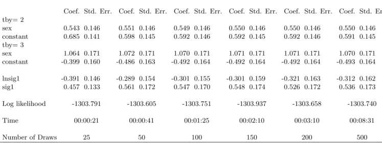
Table 1 shows the MSL results for the model with a common term of unobserved heterogeneity. Comparing the coefficients and the log likelihood between the estimations we find that the results are fairly stable when using at least 50 draws. When using only 25 Halton draws the deviations of the coefficients from those obtained with better approximated integrals can be seen. However, even with more than 100 draws we find that results slightly differ between the number of draws; the log likelihood varies between the estimations in the first decimal place. Estimation time varies between the estimations with an acceptable approximation of the integral from 0.41 (50 draws) to 8.31 minutes (500 draws); estimation results suggest that computational time increases approximately linear with the number draws.
Comparing the results derived with simulation with those estimated with quadrature, we find that the estimation results are quite similar when the integral is reasonably well approximated. When using Gauss Hermite quadrature at least 8 quadrature points are required for integration. The log likelihood and the coefficients clearly differ between the estimation with 4 and 8 points.
Turning to the Bayesian adaptive quadrature, the picture changes. With only four quadrature points the integral seem to be reasonably well approximated as a further in-crease in quadrature points leads to very similar estimated parameters. This finding underlines the result of Rabe-Hesketh, Skrondal, and Pickles (2002) who show the com-putational advantage of the Bayesian approach relative to the classical quadrature.
For the one dimensional integral it seems that Halton based simulation performs sim-ilarly to quadrature. Relative to Gauss Hermite quadrature there seem to be hardly any difference in computational time for a comparable degree of accuracy. The Bayesian ap-proach leads to more stable results with 4 quadrature points, computation time however is higher.
[Table 3 and 4 about here]
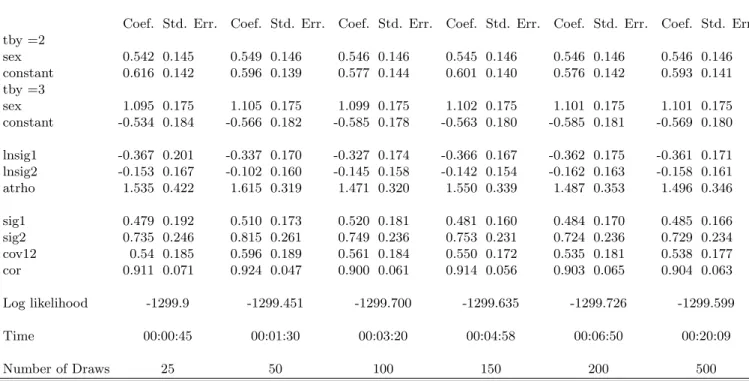
In the following the complexity of the estimation increases by allowing the unobserved heterogeneity to differ between the alternatives. Here the advantage of computational time of Halton based simulation over Gauss Hermite quadrature becomes evident. With at least 100 draws, coefficients and the log likelihood become relatively stable. For 100 draws the estimation takes more than 3 minutes. For a comparable level of integral ap-proximation Gauss Hermite quadrature requires more than 11.5 minutes. Results from MSL become more stable with 200 and 500 draws. The estimation with 200 draws takes less than 7 minutes and the one with 500 draws about 20 minutes. When doubling the number of quadrature points for the Gauss hermite approach computational time approxi-mately quadruples (50 minutes) and the results are similar to the results from the adaptive quadrature.
With adaptive quadrature, again 4 points are sufficient for approximation of the inte-gral. Results hardly change with a higher number of quadrature points. Computational time with four points is about 8 minutes. Relative to simulation, Bayesian quadrature leads to more robust results. However, using simulation with 100 draws it is possible to approximate the integral such that coefficients and the log likelihood are approximately stable in less than 3.5 minutes. Here the trade off between computational time and accu-racy becomes evident. Halton based simulation leads to results in less computational time whereas Bayesian quadrature provides results that are more stable.
From a practical point of view, the implementation of MSL based on Halton sequences is relatively simple and has significant advantages in computational time if it is compared to Gauss Hermite quadrate and simulation based on pseudo-random sequences, not re-ported here. This is in particular true for higher dimensional integrals. In comparison to adaptive quadrature our routine seems to be less stable. However, given the advantage of computational time Halton based MSL could be the adequate model choice. The time advantage becomes even more important when sample size or the dimension of the integral increases.8
Therefore we recommend the presented routine as an alternative to the quadrature approach implemented ingllamm. Moreover, the principles of our routine can be a useful starting point for the evaluation of likelihood functions which are not pre-programmed in Stata and involve a multivariate normal distribution of the unobserved heterogeneity.
8A possibility to reduce the trade off between estimation time and accuracy might be Bayesian
sim-ulation. Train (2003) suggests to employ Bayesian simulation instead of classical MSL as the Bayesian method leads to consistent estimates even with a fixed number of draws.
5
Conclusion
In this paper we have suggested a Stata routine for multinomial logit models with un-observed heterogeneity using maximum simulated likelihood based on Halton sequences. The routine refers to a model with two random intercepts, but can easily be extended to models with a higher dimension. Further extensions of the presented code are possible, examples are Haan (2005), estimating a dynamic conditional logit model or Uhlendorff (2006), estimating a dynamic multinomial logit model with endogenous panel attrition.
Using multilevel data about schooling we compare the performance of our code to the Stata program gllamm; gllammnumerically approximates integrals using classical Gauss Hermite quadrature and Bayesian adaptive quadrature. The comparison leads to the conclusion that estimation by MSL provides approximately the same estimation results as estimation with Gauss Hermite quadrature or adaptive quadrature. In comparison to classical quadrature, simulation markedly reduces computational time when a higher dimensional integral needs to be approximated. However, relative to the Bayesian method the advantage of simulation vanishes in our example. Adaptive quadrature leads to very stable results with only a few quadrature points (four points). Estimations with 100 draws are less stable but lead to qualitatively the same results and take roughly half of the estimation time. This finding underlines the trade off between computational time and accuracy of the results which becomes very important if estimation takes not some minutes but some hours or days.
6
Acknowledgement
This project is funded by the German Science Foundation (DFG) in the priority program ”Potentials for more flexibility on heterogenous labor markets” (projects STE 681/5-1 and ZI 302/7-1). We would like to thank David Drukker, Stephen Jenkins, Oswald Haan, and Katharina Wrohlich for valuable comments and suggestions.
References
Bhat, C.(2001): “Quasi-random maximum simulated likelihood estimation of the mixed
multinomial logit model,”Transportation Research B, 35, 677–693.
Cameron, C.,andP. Trivedi(2005): Microeconometrics. Cambridge University Press,
New York.
Cappellari, L.,andS. Jenkins(2003): “Multivariate probit regression using simulated
maximum likelihood,”The Stata Journal, 3, 278–294.
(2006): “Calculation of multivaraite normal probabilities by simulation,”mimeo.
Gould, W., J. Pitbaldo, and W. Sribney (2003): Maximum Likelihood Estimation
with Stata. Stata Corporation, Texas.
Haan, P.(2005): “State Dependence and Female Labor Supply in Germany: The
Exten-sive and the IntenExten-sive Margin.,”DIW Discussion Paper, 538.
Rabe-Hesketh, S., A. Skrondal, and A. Pickles (2002): “Reliable estimation of
generalised linear mixed models using adaptive quadrature,” The Stata Journal, 2, 1– 21.
(2004): “GLLAMM Manual, Technical Report,” U.C. Berkeley Division of
Bio-statistics Working Paper Series, Working Paper 160.
Skrondal, A., and S. Rabe-Hesketh (2005): Multilevel and Longitudinal Modelling
Using Stata. Stata Press, College Station, Texas.
Train, K. (1999): “Halton Sequences for Mixed Logit,” Working Paper, available from
http://elsa.berkeley.edu/wp/train0899.pdf.
Train, K.(2003): Discrete Choice Models using Simulation. Cambridge University Press,
Cambridge, UK.
Uhlendorff, A. (2006): “From no pay to low pay and back again? Low pay dynamics
Table 1: One random intercept: Maximum Simulated Likelihood
Coef. Std. Err. Coef. Std. Err. Coef. Std. Err. Coef. Std. Err. Coef. Std. Err. Coef. Std. Err. tby= 2 sex 0.543 0.146 0.551 0.146 0.549 0.146 0.550 0.146 0.550 0.146 0.550 0.146 constant 0.685 0.141 0.598 0.145 0.592 0.146 0.592 0.145 0.592 0.146 0.591 0.145 tby= 3 sex 1.064 0.171 1.072 0.171 1.070 0.171 1.071 0.171 1.071 0.171 1.070 0.171 constant -0.399 0.160 -0.486 0.163 -0.492 0.164 -0.492 0.164 -0.492 0.164 -0.493 0.164 lnsig1 -0.391 0.146 -0.289 0.154 -0.301 0.155 -0.301 0.159 -0.321 0.163 -0.312 0.162 sig1 0.457 0.133 0.561 0.172 0.547 0.170 0.548 0.174 0.526 0.172 0.536 0.173 Log likelihood -1303.791 -1303.605 -1303.751 -1303.937 -1303.658 -1303.740 Time 00:00:21 00:00:41 00:01:25 00:02:10 00:03:10 00:08:31 Number of Draws 25 50 100 150 200 500 Numbers of Observations: 3939. Source: http://www.gllamm.org/jspmix.dat
Table 2: One random intercept: Gauss Hermite and Adaptive Quadrature
Coef. Std. Err. Coef Std. Err. Coef. Std. Err. Coef. Std. Err. Coef. Std. Err. Coef. Std. Err. tby= 2 sex 0.553 0.146 0.554 0.146 0.549 0.146 0.550 0.146 0.550 0.146 0.550 0.146 constant 0.693 0.146 0.619 0.155 0.593 0.147 0.594 0.145 0.594 0.146 0.594 0.146 tby= 3 sex 1.074 0.171 1.075 0.171 1.070 0.171 1.071 0.171 1.071 0.171 1.071 0.171 constant -0.391 0.165 -0.465 0.172 -0.492 0.166 -0.490 0.163 -0.491 0.164 -0.491 0.164 sig1 0.398 0.101 0.564 0.181 0.530 0.166 0.551 0.178 0.543 0.175 0.544 0.175 Log likelihood -1305.189 -1303.681 -1303.843 -1303.802 -1303.804 -1303.804 Time 00:00:21 00:00:46 00:01:10 00:01:24 00:01:42 00:03:12 Quad. Points 4 8 16 4 (Adaptive) 8 (Adaptive) 16 (Adaptive)
Numbers of Observations: 3939.
Source: http://www.gllamm.org/jspmix.dat
Table 3: Two random intercepts: Maximum Simulated Likelihood
Coef. Std. Err. Coef. Std. Err. Coef. Std. Err. Coef. Std. Err. Coef. Std. Err. Coef. Std. Err. tby =2 sex 0.542 0.145 0.549 0.146 0.546 0.146 0.545 0.146 0.546 0.146 0.546 0.146 constant 0.616 0.142 0.596 0.139 0.577 0.144 0.601 0.140 0.576 0.142 0.593 0.141 tby =3 sex 1.095 0.175 1.105 0.175 1.099 0.175 1.102 0.175 1.101 0.175 1.101 0.175 constant -0.534 0.184 -0.566 0.182 -0.585 0.178 -0.563 0.180 -0.585 0.181 -0.569 0.180 lnsig1 -0.367 0.201 -0.337 0.170 -0.327 0.174 -0.366 0.167 -0.362 0.175 -0.361 0.171 lnsig2 -0.153 0.167 -0.102 0.160 -0.145 0.158 -0.142 0.154 -0.162 0.163 -0.158 0.161 atrho 1.535 0.422 1.615 0.319 1.471 0.320 1.550 0.339 1.487 0.353 1.496 0.346 sig1 0.479 0.192 0.510 0.173 0.520 0.181 0.481 0.160 0.484 0.170 0.485 0.166 sig2 0.735 0.246 0.815 0.261 0.749 0.236 0.753 0.231 0.724 0.236 0.729 0.234 cov12 0.54 0.185 0.596 0.189 0.561 0.184 0.550 0.172 0.535 0.181 0.538 0.177 cor 0.911 0.071 0.924 0.047 0.900 0.061 0.914 0.056 0.903 0.065 0.904 0.063 Log likelihood -1299.9 -1299.451 -1299.700 -1299.635 -1299.726 -1299.599 Time 00:00:45 00:01:30 00:03:20 00:04:58 00:06:50 00:20:09 Number of Draws 25 50 100 150 200 500 Numbers of Observations: 3939. Source: http://www.gllamm.org/jspmix.dat
Table 4: Two random intercepts: Gauss Hermite and Adaptive Quadrature
Coef. Std. Err. Coef. Std. Err. Coef. Std. Err. Coef. Std. Err. Coef. Std. Err. Coef. Std. Err. tby =2 sex 0.548 0.145 0.551 0.146 0.546 0.146 0.547 0.146 0.546 0.146 0.546 0.146 constant 0.668 0.142 0.621 0.142 0.595 0.141 0.598 0.140 0.597 0.141 0.597 0.141 tby =3 sex 1.104 0.175 1.105 0.175 1.101 0.175 1.102 0.175 1.101 0.175 1.101 0.175 constant -0.480 0.181 -0.539 0.181 -0.567 0.181 0.564 0.180 -0.565 0.180 -0.565 0.180 sig1 0.352 0.098 0.504 0.169 0.480 0.168 0.489 0.171 0.488 0.170 0.488 0.170 sig2 0.596 0.169 0.752 0.238 0.730 0.234 0.743 0.240 0.739 0.238 0.738 0.238 cov 0.406 0.108 0.560 0.180 0.537 0.177 0.547 0.182 0.545 0.181 0.545 0.181 cor 0.887 - 0.910 - 0.907 - 0.908 - 0.908 - 0.908 -Log likelihood -1300.950 -1299.482 -1299.681 -1299.663 -1299.664 -1299.665 Time 00:02:47 00:11:38 00:47:41 00:08:16 00:30:38 02:03:12 Quad. Points 4 8 16 4 (Adaptive) 8 (Adaptive) 16 (Adaptive)
Numbers of Observations: 3939.