This is a repository copy of Classification tree methods for panel data using wavelet-transformed time series.
White Rose Research Online URL for this paper: http://eprints.whiterose.ac.uk/131479/
Version: Accepted Version
Article:
Zhao, X, Barber, S orcid.org/0000-0002-7611-7219, Taylor, CC
orcid.org/0000-0003-0181-1094 et al. (1 more author) (2018) Classification tree methods for panel data using wavelet-transformed time series. Computational Statistics and Data Analysis, 127. pp. 204-216. ISSN 0167-9473
https://doi.org/10.1016/j.csda.2018.05.019
© 2018 Elsevier B.V. This manuscript version is made available under the CC-BY-NC-ND 4.0 license http://creativecommons.org/licenses/by-nc-nd/4.0/
Reuse
This article is distributed under the terms of the Creative Commons Attribution-NonCommercial-NoDerivs (CC BY-NC-ND) licence. This licence only allows you to download this work and share it with others as long as you credit the authors, but you can’t change the article in any way or use it commercially. More
information and the full terms of the licence here: https://creativecommons.org/licenses/
Takedown
If you consider content in White Rose Research Online to be in breach of UK law, please notify us by
Classification tree methods for panel data using
wavelet-transformed time series
Xin Zhaoa, Stuart Barbera1, Charles C Taylora, Zoka Milanb a
School of Mathematics, University of Leeds, U.K.
b
King’s College Hospital Trust, London, U.K.
Abstract
Wavelet-transformed variables can have better classification performance for panel data than using variables on their original scale. Examples are provided showing the types of data where using a wavelet-based representation is likely to improve classification accuracy. Results show that in most cases wavelet-transformed data have better or similar classification accuracy to the original data, and only select genuinely useful explanatory variables. Use of wavelet-transformed data provides localized mean and difference variables which can be more effective than the original variables, provide a means of separating “signal” from “noise”, and bring the oppor-tunity for improved interpretation via the consideration of which resolution scales are the most informative. Panel data with multiple observations on each individual require some form of aggregation to classify at the individual level. Three different aggregation schemes are presented and compared using simulated data and real data gathered during liver transplantation. Methods based on aggregating individual level data before classification outperform methods which rely solely on the combining of time-point classifications.
Keywords: CART, MODWT, panel data, noise exclusion
1. Introduction
We often encounter data containing multiple time series variables for organisa-tions or individuals that need classification, especially in areas such as economics, finance, marketing, medicine and biology. It can also be important to determine which of the time series are useful in performing the classification; interpreting this
1
information can be highly useful in investigating the relationships between the vari-ables and the class labels.
Our interest in this problem was motivated by data collected on patients un-dergoing liver transplant surgery. Each patient is classified into one of two groups, according to whether they did or did not use beta-blocker medication. During the operation, monitoring took place for several variables such as heart rate and sys-tolic blood pressure, with data recorded once every heartbeat. However, equivalent problems arise in many different contexts.
Denote the data asAn,k,tfor individual (or organisation)n= 1,2, . . . , N, variable
k= 1,2, . . . , K, and timet = 1,2, . . . , Tn, allowing the length of the time series to be
different for each individual. Thus, for thenth individual, the data can be expressed
as a Tn×K matrix An,·,·= An,1,1 · · · An,K,1 An,1,2 · · · An,K,2 ... . .. ... An,1,Tn · · · An,K,Tn .
The full data can be written as a
N P n=1 Tn×K matrix A, where AT = AT 1,·,· A T 2,·,· · · · A T N,·,· .
We refer to such explanatory data as panel (or longitudinal) data. The response variable Y is the group that each individual belongs to, which we write as a vector
yT =yT1,· y T 2,· · · · y T N,· ,
whereyn,· has Tn identical values, defined by (yn,1, yn,2, . . . , yn, Tn).
Difficulties in analysing such datasets include: (1) unequal values of Tn; (2)
ag-gregating the panel data to provide classification for each individual; and (3) lack of independence between consecutive times.
Such data are generally subject to noise if they are collected or recorded by people or machines. Wavelet shrinkage (Donoho and Johnstone, 1994) is a popular denoising method, which is commonly used to smooth out random noise variation in signals, and we could use such methods in our application. However, even without a formal denoising step, wavelets are able to separate out “signal” from “noise”, and we use this property to improve prediction performance. We shall also see that wavelets can pick out short term fluctuations in real data which can be exploited for classification when consecutive observations lack independence. Instead of using the standard
decimated discrete wavelet transform (DWT), we use the maximal overlap discrete wavelet transform (MODWT; see, for example, Percival and Walden (2000, ch. 5)), as it is not constrained by time series lengthTn and each time point is represented at
all resolution levels of the MODWT. Equivalent translation-equivariant transforms are the non-decimated stationary wavelet transform (Nason and Silverman, 1995) and cycle-spinning (Coifman and Donoho, 1995).
For classification, we use the classification and regression tree (CART) method of Breiman et al. (1984). Using DWT (or MODWT) with CART (or other decision trees or random forests) in time series data has already been considered (Alickovic and Subasi, 2016; Gokgoz and Subasi, 2015; Upadhyaya and Mohanty, 2016), as have other classification methods (Maharaj and Alonso, 2007, 2014) but, to the best of our knowledge, until now the application to panel data is quite rare. Previous authors have directly converted the wavelet representation of panel data into cross-sectional data by using summaries such as energy, standard deviation, or entropy (Zhang et al., 2015; Upadhyaya and Mohanty, 2016).
However detecting when and how MODWT can help CART in classification ac-curacy and variable selection for panel data is important. Thus, in this paper, we use CART with original and wavelet-transformed variables to classify panel data. We introduce our methodology in Section 2, and apply it to simulated panel data experiments in Section 3 before analysing our liver transplantation (LT) panel data in Section 4. Some concluding comments appear in Section 5.
2. Methodology
In this section, CART and the MODWT are introduced briefly. For more details, see Breiman et al. (1984) and Percival and Walden (2000), respectively. We then pro-pose three methods to produce individual-level classifications from panel data, which can be applied to the original data, the wavelet-transformed data, or a combination of both.
2.1. Background
The goal of CART is to construct a model that predicts the value of a response variable by learning simple decision rules inferred from data features. In our case, we use classification trees since the response variable is categorical. The model built is structured as a tree with each node representing a split of the data in that node according to the value of a single variable. The aim is to use successive decision rules to split the data in a way which makes the subset of data at each terminal node (leaf node) as pure as possible, ideally with only one class. The tree represents, therefore,
a classification rule using only those variables which are found to convey as much relevant information as possible. The tree construction process involves building and then pruning a tree. In the tree building process, we use optimization of the Gini index as our splitting criterion to choose the best explanatory variable to construct a decision at each node. Specifically, the decision rule using the selected variable at each node will determine a subset of the data which is as pure as possible, as measured by the Gini index. In the pruning process, we use ten-fold cross-validation to mitigate the tendency of CART to produce over-fitted models. Overall, then, CART is used to construct a classification rule which incorporates a variable selection stage as part of the construction process.
In the MODWT, we use the Haar scaling function φ and waveletψ, where
φ(τ) = 1 τ ∈[0,1) 0 else, and ψ(τ) = 1 τ ∈[0,1/2) −1 τ ∈[1/2,1) 0 else. (1)
By using dilation and translation, we obtain the scaling function and wavelet at location l and resolution level j:
φj,l(τ) = 2j/2φ 2j(τ −l)
and ψj,l(τ) = 2j/2ψ 2j(τ −l)
,
where j = 0,1, . . . , J, for J = ⌊log2n⌋, and l = 0,1, . . . , n−1. Note that φj,l and
ψj,l are compactly supported on Ij,l =
2−jl,2−j(l + 1). When j = 0, the scaling
coefficients are actually the original time series values.
To represent our data in terms of the Haar wavelet basis, we compute scaling coefficients sj,l defined by sj,l =hAn,k,·, φj,li= Tn X t=1 An,k,tφj,l(t/Tn) = 2j/2 X t/Tn∈Ij,l An,l,t.
The Haar wavelet coefficientsdj,k can then be calculated as dj,l =sj−1,l−sj,l; hence
coefficients ofφj,l andψj,l represent local averages and contrasts, respectively, in the
intervalIj,l. To interpret these coefficients, note that whenj is small the
correspond-ing scalcorrespond-ing and wavelet functions are highly localized at that fine scale, representcorrespond-ing brief transient effects. Conversely, when j is large, they represent lower frequency activity at a coarser scale.
The scaling coefficients s and wavelet coefficients d are treated as new vari-ables which we can use for classification. We denote the wavelet transformed data
MODWT(An,k,·) for variable k on individual n as the Tn×2J matrix Wn,k,·, where Wn,k,·= Wd1 n,k,1 · · · W dj n,k,1 W s1 n,k,1 · · · W sj n,k,1 Wd1 n,k,2 · · · W dj n,k,2 W s1 n,k,2 · · · W sj n,k,2 ... . .. ... ... . .. ... Wd1 n,k,Tn · · · W dj n,k,Tn W s1 n,k,Tn · · · W sj n,k,Tn .
The wavelet transformed explanatory data are then
W = W1,1,· · · · W1,K,· W2,1,· · · · W2,K,· ... . .. ... WN,1,· · · · WN,K,· . 2.2. Classification methods
Since we wish to classify individuals, but are dealing with panel data, we can not use the predictions from CART directly as these classify each time point separately. We need to combine the information either by combining time-point level predic-tions or aggregating data first and then performing classification for individuals. We now propose several methods to classify individuals based on panel data, which we illustrate in terms of the original data A. Equivalently, these methods can also be applied to the wavelet-transformed dataW, or indeed to a combination of AandW. For simplicity, each of the methods is described in terms of a binary classification, but is easily generalized to more than two groups.
2.2.1. Method 1: prediction aggregation after classification
Using CART, we can obtain the predicted class ˆyn,t of each individual for every
time point t= 1, . . . , Tn and schematically we have
An,·,·= An,1,1 · · · An,K,1 An,1,2 · · · An,K,2 ... . .. ... An,1,Tn · · · An,K,Tn →yˆn,. = ˆ yn,1 ˆ yn,2 ... ˆ yn,Tn .
For individual n, we compute the proportion of time points which were classified as group 1, Pn= 1 Tn Tn X t=1 I{yˆn,t= 1},
where we define the indicator variable
I{yˆn,t = 1}=
1 if ˆyn,t = 1
0 if ˆyn,t = 2.
We use the prediction at each time point to predict the class of individual n:
An,·,·→yˆn=
1 ifPn>a
2 otherwise, where the best split pointa is found by using a global search.
2.2.2. Method 2: predictions based on time-point level and individual level CART Here, we first construct a classification tree as in Method 1. Variable k′
is used in this classification tree, where k′
∈ {1,2, . . . , K′
}, making a total of K′
newly renumbered variables. So the data set used in this tree becomes
A′
n,.,. = [An,k′,t]Tn×K′.
For each observed value of each of these variables, we first use the tree to derive the probability of classifying an observation as being from group 1, based on the subtree descending from that observation.
Consider variablek′
. To compute the derived probabilities, we inspect the nodes in the tree where variable k′
is used. In a node, with split point η, observations satisfying An,k′,t < η are directed to one sub-tree, while those satisfying An,k′,t > η
are directed to a different sub-tree. In each sub-tree, we find the proportion classified as group 1, and replaceAn,k′,t by this probability, which we denote as Pn,k′,t.
For example, for An,k′,t, if An,k′,t > η, then
Pn,k′,t =PA
n,k′,.>η,
wherePAn,k′,.>η is the proportion classified as group 1 for variablek
′
in that sub node satisfying An,k′,. > η.
If variablek′
is used in more than one node, we take the product of the probabil-ities (note that k′
∈ {1,2, . . . , K′
} implies that variable k′
must be used in at least one node). For example, if variable k′ appeared twice, with thresholds η
1 and η2,
then
Pn,k′,t=PA
n,k′,.>η1 ·PAn,k′,.>η2,
where PAn,k′,.>η1 and PAn,k′,.>η2 are the proportions classified as group 1 for variable
k′
This whole process is repeated for each k′
∈ {1,2, . . . , K′
} in turn, converting each time series of observed values to a vector of proportions and finally, from A′
n,.,.,
we get
Pn,.,. = [Pn,k′,t]K′×Tn.
Then we take the mean and standard deviation of these empirical probabilities as new variables to use in a “second-stage” CART. (Of course, other summaries could be used.) Schematically, we have
Pn,·,·= Pn,1,1 · · · Pn,K′,1 Pn,1,2 · · · Pn,K′,2 ... . .. ... Pn,1,Tn · · · Pn,K′,Tn (2) ւց ւց Pn,k,(m)· = h Pn,(m1,)·, P (sd) n,1,· · · · P (m) n,K′,·, P (sd) n,1,· i .
We then calculate the mean and standard deviation matrix for all individuals and variables as a cross sectional data
e P = P1(,m1,.) · · · P1(,Km)′,. P (sd) 1,1,. · · · P (sd) 1,K′,. P2(,m1,.) · · · P2(,Km)′,. P (sd) 2,1,. · · · P (sd) 2,K′,. ... . .. ... ... . .. ... PN,(m1),. · · · PN,K(m)′,. P (sd) N,1,. · · · P (sd) N,K′,. . (3)
After that, we apply CART to Pe, and get the predicted value for each individual:
e P = P1(,m1,.) · · · P1(,Km)′,. P (sd) 1,1,. · · · P (sd) 1,K′,. P2(,m1,.) · · · P2(,Km)′,. P (sd) 2,1,. · · · P (sd) 2,K′,. ... . .. ... ... . .. ... PN,(m1),. · · · PN,K(m)′,. P (sd) N,1,. · · · P (sd) N,K′,. →yˆ= ˆ y1 ˆ y2 ... ˆ yN . (4)
Note that in this second stage, each individual has just one mean and one standard deviation value corresponding to each of the variables in that tree, hence there is only one predicted class for each individual.
2.2.3. Method 3: data aggregation before classification
Here, we aggregate the original data for each individual into a small number of summaries for each variable — chosen to reflect the nature of the data — to form
individual level cross-sectional data, and then use CART directly. In our implemen-tation, we use the mean A(n,k,m)· and standard deviation A
(sd)
n,k,· of variable k for each
individualn An,k,t to construct cross sectional data
e
A= [A(m), A(sd)]N×2K,
where A(m) = [A(m)
n,k,·]N×K and A(sd) = [A(n,k,sd)·]N×K. The process is the same as in
Equations (2) to (4), but applied to dataA rather than probabilities P.
3. Simulation study
We now explore the performance of Methods 1–3 using both original and wavelet-transformed data in a simulation study, before applying the methods to our LT data in Section 4. We conduct 100 replicate trials for each simulation. For every trial, we generate new data on N individuals and then split the N individuals into training and test sets, with 0.8N individuals used for training and the remaining data used to assess performance. All three methods are used for each dataset.
In this section, we investigate: (1) whether wavelet variables have better per-formance in classification than the original variables; (2) which variables are more important in the tree; (3) which of the proposed methods perform better in differ-ent circumstances. Our criteria are prediction accuracy and the ability to correctly identify informative variables.
All computations were performed in R (R Core Team, 2014), using the
pack-ages rpart (Therneau et al., 2014) for constructing classification trees and waveslim
(Whitcher, 2013) for wavelet decomposition. 3.1. Data generation
We generate panel data with two groups, comprising a total of N = 300 individ-uals. For each individual, there are 10 “time series” variables. Five of these variables (V1–V5) are informative, having different distributions in the two groups, while the
remainder (V6–V10) are identically distributed across both groups and referred to as
redundant variables. Details of the variables’ models, distributions and parameters are shown in Table 1.
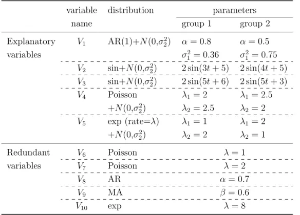
For each informative variable, the parameters of the models are chosen so that the first two moments are identical for the two groups. The five explanatory variables follow an AR process (V1), sine models (V2 and V3), Poisson (V4) and exponential
(V5) distributions, so we have both autocorrelated and independent variables. We
independently generateTs
n ∼U(Tn/4,3Tn/4) as a “change point” for each individual
Table 1: Simulation variables and parameters. Variables V1–V5 are contaminated at rate θ by
normally distributed noise which has the same mean and variance as the variable in question.
variable distribution parameters
name group 1 group 2
Explanatory V1 AR(1)+N(0,σ22) α = 0.8 α= 0.5
variables σ2
1 = 0.36 σ21 = 0.75
V2 sin+N(0,σ22) 2 sin(3t+ 5) 2 sin(4t+ 5)
V3 sin+N(0,σ22) 2 sin(5t+ 6) 2 sin(5t+ 3)
V4 Poisson λ1 = 2 λ1 = 2.5 +N(0,σ2 2) λ2 = 2.5 λ2 = 2 V5 exp (rate=λ) λ1 = 1 λ1 = 2 +N(0,σ2 2) λ2 = 2 λ2 = 1 Redundant V6 Poisson λ= 1 variables V7 Poisson λ= 2 V8 AR α= 0.7 V9 MA β = 0.6 V10 exp λ= 8
same distribution but with different parameters. Noise is added to V1–V5 in two
ways. Firstly, we add Gaussian white noise ǫt∼ N(0, σ22), and we also contaminate
the data by making random replacements at rateθwithN(µ, σ2), whereµandσ2 are
the theoretical mean and variance of the variable in question. These data generation methods ensure that the marginal distribution for each explanatory variable between two groups is the same, while the joint distribution is different between two groups. In order to assess the influence of noise levels and group balance on classification accuracy and selection of explanatory variables, we conduct simulations under dif-ferent circumstances with noise level 06σ2 620, contamination rate 0.16θ 60.8
and the number of individuals in group 1 ranging from 150 to 270, with the total number N = 300 fixed.
After generating our data, we carry out the wavelet transform on these variables, using the Haar wavelet. Then, we use the original and wavelet-transformed data for our simulation experiment. We conduct 100 replicate trials for each experiment. 3.2. Separate analysis for each explanatory variable
3.2.1. Classification accuracy
In order to tell which explanatory variable is most effective in classification, we built classification trees with only one informative explanatory variable at a time, replacing the other four informative variables with standard Gaussian white noise N(0, σ2 = 1). This provides a check that the CART methodology is correctly
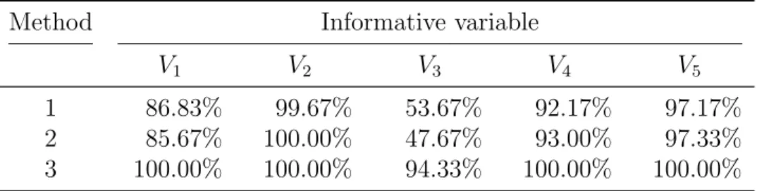
select-ing informative variables while ignorselect-ing variables that contain no useful information. In each case, classification accuracy for the original variables on the test data is gen-erally around 50%. However, Table 2 shows that, for wavelet variables, it is gengen-erally above 85% except for V3, which is noticeably lower. In particular, variable V2 is the
most informative. We attribute this to the wavelet coefficients distinguishing the different frequencies of V2 in the two groups. Method 3 is usually the best method
due to the aggregation over time points effectively averaging out random variation, giving a cleaner picture of the differences between the groups.
3.2.2. Interpretation of scale choice
A further advantage of using wavelet-transformed data is the added insight which can sometimes be gained by considering which scales are used in the classification. In order to illustrate clearly, we simplify parameters by fixing Tn = 768 and Tns =
Tn/2 = 384, and do not add white noise to the explanatory variables but for V2–V5,
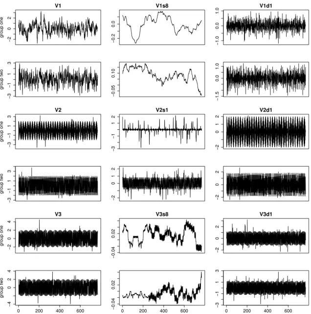
we still randomly replace 10% of generated observations with noise. Figures 1–3 show examples of the time series generated and plots of those wavelet-transformed variables which were most commonly selected as containing useful information by
Table 2: Classification accuracy when using wavelet-transformed version of each of the informative variables in isolation.
Method Informative variable
V1 V2 V3 V4 V5
1 86.83% 99.67% 53.67% 92.17% 97.17%
2 85.67% 100.00% 47.67% 93.00% 97.33%
3 100.00% 100.00% 94.33% 100.00% 100.00%
CART. We note that CART can easily detect differences in the mean level of a variable with a single split, and can also partially detect increased variance by two splits.
V1 ForV1, the main variables chosen weres8 (representing smoothing over a window
of 28 = 256 time points) and d
1 (the difference between successive
observa-tions). Recall that V1 follows an AR(1) model with autoregressive parameter
α= 0.8 in group 1 andα= 0.5 in group 2, so the short-term autocorrelation is substantially higher in group 1. Using the raw data does not access this infor-mation, but it is detected by the local averages in V1s8 and local fluctuations
inV1d1.
V2 ForV2, the frequency difference in the sine function is detected by both V2s1 and
V2d1.
V3 The sine function in the two groups differs only by a phase translation along the
time axis. This is not easily recognized as it does not affect the autocorrela-tion or frequency characteristics which are encoded in the wavelet-transformed variables. Indeed, Methods 1 and 2 fail in this case.
Method 3 still works here, but the reasons are subtle and the improvement is in fact an artefact caused by the data lengthTn not being a multiple of the cycle
length of the sine wave. This means that changing the starting point of the cycle results in one part of the cycle being slightly over-represented, illustrated in Figure 2. This effect, though small, is picked up when the V3s8 and V3d1
variables are averaged over the full time series. Since this effect will change as the relationship between the cycle length andTnchanges, we would not expect
the good performance of Method 3 to be relied upon for variables like V3 in
−2 0 2 V1 group one −0.2 0.0 V1s8 −1.0 0.0 1.0 V1d1 −3 −1 1 3 group tw o −0.05 0.10 −1.5 0.0 1.0 −3 −1 1 3 V2 group one −3 −1 1 2 V2s1 −2 0 1 2 V2d1 −3 −1 1 3 group tw o −2 0 1 2 −2 0 2 −2 0 2 4 V3 group one −0.04 0.02 V3s8 −2 0 2 V3d1 0 200 400 600 −4 0 2 4 group tw o 0 200 400 600 −0.04 0.02 0 200 400 600 −3 −1 1 3
Figure 1: Wavelet transformed information forV1–V3 for individual one separately in group 1 and
−2 0 1 2 V3 group one −0.15 0.00 0.15 V3s4 −1.0 0.0 1.0 V3d1 5 10 15 20 −2 0 1 2 group tw o 5 10 15 20 −0.10 0.05 5 10 15 20 −1.0 0.0 1.0
Figure 2: An example ofV3 for group 1 and group 2 with time length 20 and without noise added
and contamination rate.
0 2 4 6 V4 group one 1.8 2.2 2.6 V4s8 −0.1 0.2 0.4 V4d8 0 2 4 6 8 group tw o 2.0 2.4 −0.3 0.0 0.2 −1 1 3 5 V5 group one 0.5 0.8 1.1 V5s8 −0.2 0.0 V5d8 0 200 400 600 0 2 4 6 8 group tw o 0 200 400 600 0.5 0.7 0.9 0 200 400 600 −0.1 0.1
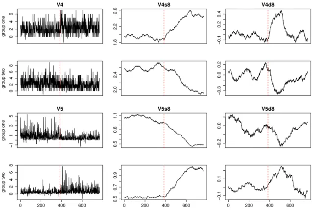
Figure 3: Wavelet transformed information forV4–V5 for individual one separately in group 1 and
V4, V5 These variables are each the same mixture when aggregated over time points,
but differ in which parts of the signal they are slightly higher and lower. Vi-sually, the difference is clear in thes8 variables which form localized averages.
This difference is lost when aggregated along the time axis, as happens with the original variables. However, the differences at scale 8 are extremely helpful here as they record larger positive (negative) values when there is an increase (de-crease) in the local mean. In addition, the taking of localized means effectively averages out the white noise.
These differences could be detected from the original variables, but care would be needed to compute a summary statistic that would encode the differences between groups, especially if the location of the change pointTs
n is not known.
Although the examples in Figure 3 have Ts
n =Tn/2 for simplicity, the
wavelet-transformed variables will detect the presence of an increase or decrease in the localized means adaptively regardless of the best scale to average over or location of the change point.
3.3. Simulation with all explanatory variables included 3.3.1. Ideal circumstance
In ideal circumstances, we have noise level σ2 = 0, a low contamination rate of
θ= 0.1 and equal group sizes. We also construct situations in which CART works for the original data, by adding an offsetδ = 0.2 to all observations of variables V1−V5
in group 1, making the expectation of these variables higher in group 1.
Corresponding results in Table 3 show that using CART with the original data cannot distinguish the two groups using Methods 1 and 2, as it simply uses the default tree (classifying all individuals into the majority group). It is a little better when using Method 3, with a prediction accuracy of 36.7/60 and detecting explanatory variables V1, V3. However, using wavelet transformed data results in nearly 100%
prediction accuracy. The explanatory variables and scales used are consistent with those in Figures 1–3. For Methods 1–2, V2 is still the best explanatory variable,
followed by V5 (and V1). For Method 3, V1,V5 and V2 are all quite good.
When we use the increase in mean level, it is obvious that original data and wavelet-transformed data share identical accuracy. When explanatory variables have obvious mean-levels differences between two groups, wavelet-transformed variables have the same good performance as original data. In terms of variable choice, CART with original data generally chooses all the explanatory variables especially their means, and still selects redundant variables in some cases. However, CART with wavelet-transformed variables is more parsimonious while retaining excellent accu-racy and is less likely to include redundant variables.
Table 3: Testing accuracy results with noise levelσ2 = 0, contamination rate θ = 0.1 and equal
group sizes of 150. Accuracy is the number of correctly classified individuals from a training set of 60, averaged over 100 replicate simulations. Entries – indicate that no splitting was done.
Method Accuracy (/60, sd) original wavelet
Original Wavelet variables* redundant** variables*
Offset δ = 0 1 30.0(0.00) 59.7(0.64) – – V2 V5 V1 2 30.0(0.00) 60.0(0.00) – – V2 V5 3 36.7(3.90) 59.5(0.83) V1 V3 (m sd) yes V1 V5 V2 Offset δ = 0.2 1 59.8(0.46) 59.6(0.79) V5–V1 yes V2 V3 2 60.0(0.00) 59.9(0.34) V4 V5 (m sd) no V2 V5 V3 3 60.0(0.10) 59.7(0.59) V1–V5 (m) no V5 V2
* Main variables in the first six important variables from CART. ** Whether redundant variables are used by CART.
No redundant variables were selected by CART using wavelet variables.
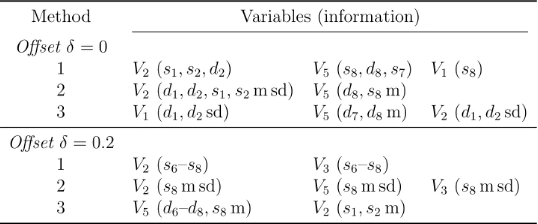
Table 4: Choice of variable, resolution level and wavelet or scaling coefficient when applying CART to wavelet-transformed simulated data.
Method Variables (information)
Offset δ= 0 1 V2 (s1, s2, d2) V5 (s8, d8, s7) V1 (s8) 2 V2 (d1, d2, s1, s2m sd) V5 (d8, s8m) 3 V1 (d1, d2sd) V5 (d7, d8m) V2 (d1, d2sd) Offset δ= 0.2 1 V2 (s6–s8) V3 (s6–s8) 2 V2 (s8m sd) V5 (s8m sd) V3 (s8m sd) 3 V5 (d6–d8, s8m) V2 (s1, s2m)
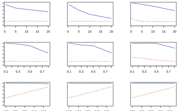
0 5 10 15 20 0.4 0.6 0.8 1.0 Method 1 noise le v el accur acy 0 5 10 15 20 Method 2 0 5 10 15 20 Method 3 0.1 0.3 0.5 0.7 0.4 0.6 0.8 1.0 contaminant accur acy 0.1 0.3 0.5 0.7 0.1 0.3 0.5 0.7 180 200 220 240 260 0.4 0.6 0.8 1.0 group siz e accur acy 180 200 220 240 260 180 200 220 240 260
Figure 4: Testing accuracies results for real circumstances. Blue solid lines represent results for wavelet variables and red dash lines represent that for original variables. X-axis for the first row is noise level, for the middle row is contamination rate, for the last row is group 1 size.
3.3.2. Real circumstances
We now consider changes in noise level, contamination rate and group size bal-ance. The corresponding results are shown in Figure 4. Each panel gives classifica-tion accuracy as the proporclassifica-tion of correctly classified individuals for both wavelet-transformed and original data (solid and dashed lines respectively) under a range of circumstances.
As one would expect, increasing noise or contamination levels reduces the accu-racy of the methods using wavelet-transformed data, with Method 3 being least af-fected since the aggregation over time points before classification effectively averages out noise in the wavelet coefficients before conducting the classification procedures. The classification accuracy obtained using the original data is broadly unchanged, since classification was already essentially arbitrary in this case.
Making the groups more unbalanced leaves classification using wavelet-transformed data largely unchanged, while classification using the original data appears to im-prove since predicting all individuals to be from the dominant group becomes an
increasingly effective strategy.
3.4. Alternative wavelet transform functions
In the simulation, we have used the Haar wavelet basis defined in Equation (1). There are many other choices of wavelet basis available and we have repeated our analyses with minimum-bandwidth discrete-time wavelets with filter length 4 (mb4), Daubechies wavelets with filter length 4 (db4) and Least Asymmetric wavelets with filter length 8 (la8) in the R package waveslim. Full results are not included here, but they have shown that Haar is generally better than the others in most circum-stances. Compared with la8, Haar is almost always better. When comparing Haar with mb4 and d4, Haar is better in all three methods with low noise level and low contaminant rate. When noise level and contaminant rate are high (5, 10, 20 and 0.5, 0.8 respectively), Haar is no longer the best in Methods 1 and 2 but still the best in Method 3. In most cases, Method 3 has the best performance. Therefore, due to good accuracy and the easier interpretation of the Haar wavelet, we recommend the Haar basis in practice.
4. Application to Liver Transplantation data
4.1. Data Description and Preprocessing
Liver Transplantation (LT) is a high-risk surgical treatment choice for patients suffering end-stage liver disease (Milan et al., 2016). Pre-operative treatment like beta-blockers may help reduce the surgical risk to some extent while also influencing the chance of surgical complications. For example, systolic dysfunction and low car-diac output with beta-blockers may compromise renal perfusion (Chirapongsathorn et al., 2016). So, if we can monitor variables like heart rate, systolic dysfunction and cardiac output effectively, then we may detect adverse effects earlier. We use these explanatory variables to classify patients as using or not using beta-blockers. In practice, a patient’s beta-blocker use is known before surgery, but here we classify pa-tients’ into beta-blocker use to investigate which monitoring variables are considered informative in the classification.
Data on patients undergoing LT between September 2004 and December 2011 at St James’ University Hospital, Leeds, UK, was recorded using LIDCO monitor-ing equipment (LIDCO, Cambridge, UK). The intraoperative monitormonitor-ing variables recorded are shown in Table 5; for more details, see Milan et al. (2016). After removal from the data set of some individuals with poor-quality data, there are 90 patients who used beta-blocker (group 1) and 236 patients who did not (group 2). For each patient, the data consist of a multivariate time series of length one thousand to tens of thousands.
Table 5: Monitoring variables recorded in the liver transplant (LT) data set.
Abbreviation Full name Unit
CO cardiac output L/min
CI cardiac index L/min/m2
SVR systemic vascular resistance dyne-s/cm5
SVRI systemic vascular resistance index dyne-s/cm5/m2
Sys systolic pressure mm Hg
MAP mean arterial pressure mm Hg
Dia diastolic pressure mm Hg
SV stroke volume mL/beat
SVI stroke volume index mL/m2/beat
HR heart rate beats/min
Since the number of patients in group 2 is around 2.6 times that in group 1, CART might be biased to predict new patients as being from group 2. This imbalance could be dealt with by using a cost matrix, by discarding data from the larger group, or by sampling replicate data from the smaller group. We chose the latter; after randomly sampling training and testing data from the entire data set, we triplicate the individuals from group 1 for training and testing data separately. There are then a total of 270 patients in group 1, relatively in balance with 236 patients in group 2. To investigate the robustness of our results to this procedure, we conduct the analysis twice, both with and without group size modification.
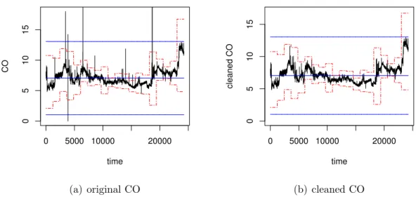
The data required considerable cleaning before classification could be attempted. There are some quite sharp increases and decreases, although variables like HR should not increase or decrease so suddenly as long as the patient is still alive. We assume that variables for each patient would not fluctuate sharply in a short time phase, and hence should remain within a limited range over a short time. Data points outside this range are regarded as outliers. There are also a non-trivial number of missing or impossible values. Firstly, we deal with data values outside the plausible range and we call this the initial filter stage. For the second stage, we will tackle data values which fluctuate sharply in a short time span and we call this the secondary filter
stage.
Initial filter Since there are outliers, we use robust statistics for cleaning. Define madn,k = median{|An,k,·−median(An,k,·)|},
the median of the absolute deviations from the median. If An,k,t is missing,
infinite or zero, or satisfies
An,k,t ∈/ [median(An,k,.)−5 madn,k, median(An,k,.) + 5 madn,k],
then we carry the last observation forward and replace An,k,t by An,k,t−1. If
t−1 = 0, then we use the median of that variable. We use the previous value for replacement due to the presence of autocorrelation and since the previous value has already been defined as non-outlying.
Secondary filter In the secondary filter stage, we make the assumption that data values would not fluctuate sharply in a short time interval equal to 1/20 of the time series length. (Other time intervals were considered, but in practice for these data, intervals of Tn/20 worked well.) We define
Qjn,k,p =jth decile of {An,k,ti+1, An,k,ti+2, . . . , An,k,ti+s},
where i = s(p− 1), s = Tn/20 and p = 1,2, . . . ,20 refers to the pth short
time phase. With Q1 and Q9 as the first and ninth deciles and d = Q9−Q1,
we replace data values An,k,t ∈/ [Q1−1.5d, Q9 + 1.5d] by An,k,t = An,k,t−1. If
t−1 = 0, then An,k,t =Q5.
After data cleaning for the whole data set, only a small proportion of the values (0.3% to 2% per variable) are changed. As an example, raw and cleaned CO data from patient 5 are shown in Figure 5.
4.2. Results
After data cleaning, we put the original and wavelet-transformed variables into our classification methods, randomly sampling 80% of the data for training and the remaining 20% for testing. To reduce sensitivity of observed classification accuracy to this sampling, we conducted 50 replicate trials for each method. The corresponding results are shown in Table 6.
Without group size adjustment, Methods 2 and 3 generally choose to split no variables and remain as default tree and Method 1 does worse than this, sometimes choosing group 1 as the main group during the time-point level tree construction process. Method 2 also has such cases, so that is why their standard deviations are high. Without these cases, they generally choose the default tree with accuracy around 45 to 46 and standard deviation around 1 and 2. These confirm that group size adjustment is needed in this case.
0 5000 10000 20000 0 5 10 15 time CO (a) original CO 0 5000 10000 20000 0 5 10 15 time cleaned CO (b) cleaned CO
Figure 5: Example of data cleaning for CO data from patient 1. Solid horizontal lines represent median and initial filter range, dashed lines represent secondary filter range.
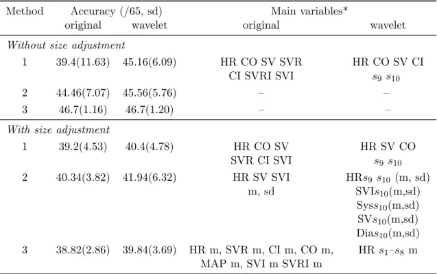
After group size adjustment, individuals in group 1 account for 53.4% of all the individuals, approximately in balance with individuals in group 2. Student’s t-test shows there are no significant differences between all three methods either for wavelet-transformed or for original data. However, accuracy from wavelet-wavelet-transformed data is slightly higher in nearly all cases. This may be due to some variables’ means in different groups being sufficiently different for decision rules using the original data to work well. When we come across data that has no significant mean difference, wavelet transform is highly recommended as its accuracy is significantly higher. Size adjustment initially seems to lower the accuracy, but it should be noted that with the balanced group sizes a default tree will now attain accuracy of 33/65. Without considering the time for wavelet transform, the computation time for Method 2 (around 7 hours per trial) is much longer than Method 3 (less than 1 second per trial). So, we find the best prediction of beta-blocker use to be achieved by using wavelet-transformed data in Method 3 with a size adjustment.
The main variables chosen are HR, SV, CO, SVR, SVI, and CI. CART based on wavelet-transformed data generally chooses smoothed variables on resolution level 9 or 10, effectively choosing to use moving-average versions of the original data. In this case, some variables have different means between the two groups (Milan et al., 2016), so CART based on original data works reasonably well, but the automatic
smoothing of the variables via the wavelet transform improves the classification. It also gives us the added interpretation that the optimal smoothing is done over a time window of 29–210 heartbeats, approximately 5–17 minutes. This finding has clinical
relevance. One of the main effects of beta-blockers is a slowing heart rate. A previous study that compared heart rates among a group of patients — both treated and not treated with beta-blockers — found a difference between two large groups with more than 10,000 measurements for each patient (Milan et al., 2016). Since clinical data during long surgical procedures were ‘noisy’, the complex statistics performed elicited the need for data smoothing. Wavelet-transformed variables have shown improved interpretation via consideration of which resolution scales are the most informative. This method can be applied to other ‘noisy’ databases in the future.
Table 6: Testing accuracy results for the LT data using Methods 1–3 with and without group size adjustment. The main variables listed are the first six important variables list output by CART.
Method Accuracy (/65, sd) Main variables*
original wavelet original wavelet
Without size adjustment
1 39.4(11.63) 45.16(6.09) HR CO SV SVR HR CO SV CI
CI SVRI SVI s9 s10
2 44.46(7.07) 45.56(5.76) – –
3 46.7(1.16) 46.7(1.20) – –
With size adjustment
1 39.2(4.53) 40.4(4.78) HR CO SV HR SV CO SVR CI SVI s9 s10 2 40.34(3.82) 41.94(6.32) HR SV SVI HRs9 s10 (m, sd) m, sd SVIs10(m,sd) Syss10(m,sd) SVs10(m,sd) Dias10(m,sd) 3 38.82(2.86) 39.84(3.69) HR m, SVR m, CI m, CO m, HR s1–s8 m
5. Conclusions and discussion
Wavelets provide a basis for automatic feature extraction methods, allowing the classification technique (CART in our case) to select from localized means and dif-ferences over a range of scales. Compared to other feature extraction methods, the initial process is not dimension reduction. Feature extraction methods such as principal component analysis (Asavaskulkeit and Jitapunkul, 2009), Locality sensi-tive hashing (Datar et al., 2004), and manifold learning (Costa and Hero, 2004; Nie et al., 2010), all aim to reduce the number of explanatory variables whilst using wavelet-transformed variables actuallyincrease the dimension by transforming orig-inal variable into detail and smoothed coefficients on different resolution levels. This can reveal hidden information which is not easy for classification trees to find using only the original data. This does mean that wavelet transformation of the data is more suitable for experiments without an excessive number of predictors, otherwise a further variable reduction step will be required and this will increase the computa-tional burden (Mazloom and Ayat, 2008; Chitaliya and Trivedi, 2010; Li and Wen, 2014).
CART, as a decision tree method, can be seen as a variable reduction method since it chooses the “best” variable to split on in each step. Compared to methods like ANN (Rowley et al., 1998), SVM (You et al., 2014) and LASSO (Roberts and Nowak, 2014), its main advantage is its ease of interpretation, although it might not achieve the same accuracy as other methods. When applying CART to wavelet-transformed data, the disadvantages of using the wavelet transform are mitigated since CART carries out a dimension reduction function. By learning which wavelet-transformed variables are more effective, we can also gain the added interpretation of which scales are important.
Compared to other feature extraction methods, the wavelet transform has its own advantages. It helps discover information hidden by noise that can not be achieved by other methods which do not provide information decomposition across different scales for one single variable. In our simulation, we have shown the effectiveness of wavelet-transformed data in CART classification where the key features of interest are changes in autocorrelation or frequency structures (our variablesV1 and V2), or
relatively small changes in mean level which occur at unknown times and are hidden by considerable noise (V4 and V5).
The scaling function we use in wavelet decomposition is the Haar wavelet, the simplest case of the compactly-supported wavelets described by Daubechies (1992). In our experience, the Haar wavelet tends to have equal or better accuracy than other choices of wavelet and has the benefit or easier interpretation. For data whose expectation and variance have some connection, such as our Poisson and
exponen-tially distributedV4 andV5, we might consider using the Haar-Fisz wavelet transform
(Fryzlewicz and Nason, 2004). Since, in real situations, we will usually not know the distribution of the time series, we generally use the Haar wavelet which is a robust all-purpose selection that allows for easy interpretation compared to more complicated wavelet bases.
We set out to produce individual-level predictions from panel data, where sim-ple application of CART produces time-point level predictions. Comparison of the different methods we used has shown that methods which perform at least some aggregation before prediction have improved performance over a naive approach of predicting at each time point and using a simple voting mechanism to aggregate these predictions. Additionally, aggregation before classification (Method 3) is com-putationally quite fast in comparison to Methods 1 and 2. So, overall, we recommend Method 3 with wavelet transformed data.
Acknowledgement
Xin Zhao is grateful for the financial support of the China Scholarship Council (CSC) during this research.
References
Alickovic, E. and Subasi, A. (2016). Medical decision support system for diagnosis of heart arrhythmia using DWT and random forests classifier, Journal of Medical
Systems 40(4): 1–12.
Asavaskulkeit, K. and Jitapunkul, S. (2009). The color face hallucination with the linear regression model and MPCA in HSV space, 2009 16th International
Con-ference on Systems, Signals and Image Processing, IEEE, pp. 1–4.
Breiman, L., Friedman, J., Stone, C. J. and Olshen, R. A. (1984). Classification and
Regression Trees, Wadsworth, Belmont.
Chirapongsathorn, S., Valentin, N., Alahdab, F., Krittanawong, C., Erwin, P. J., Murad, M. H. and Kamath, P. S. (2016). Nonselective β-blockers and survival in patients with cirrhosis and ascites: A systematic review and meta-analysis,Clinical
Gastroenterology and Hepatology .
Chitaliya, N. G. and Trivedi, A. (2010). Feature extraction using wavelet-pca and neural network for application of object classification & face recognition,Computer
Engineering and Applications (ICCEA), 2010 Second International Conference on,
Coifman, R. R. and Donoho, D. L. (1995). Translation-invariant de-noising,inA. An-toniadis and G. Oppenheim (eds), Wavelets and Statistics, Vol. 103 of Lecture
Notes in Statistics, Springer-Verlag, New York, pp. 125–150.
Costa, J. A. and Hero, A. O. (2004). Geodesic entropic graphs for dimension and entropy estimation in manifold learning, IEEE Transactions on Signal Processing
52(8): 2210–2221.
Datar, M., Immorlica, N., Indyk, P. and Mirrokni, V. S. (2004). Locality-sensitive hashing scheme based on p-stable distributions, Proceedings of the Twentieth
An-nual Symposium on Computational Geometry, ACM, pp. 253–262.
Daubechies, I. (1992). Ten Lectures on Wavelets, SIAM, Philadelphia.
Donoho, D. L. and Johnstone, J. M. (1994). Ideal spatial adaptation by wavelet shrinkage, Biometrika81(3): 425–455.
Fryzlewicz, P. and Nason, G. P. (2004). A Haar-Fisz algorithm for Poisson intensity estimation, Journal of Computational and Graphical Statistics 13(3): 621–638. Gokgoz, E. and Subasi, A. (2015). Comparison of decision tree algorithms for EMG
signal classification using DWT,Biomedical Signal Processing and Control18: 138– 144.
Li, S. and Wen, J. (2014). A model-based fault detection and diagnostic methodology based on PCA method and wavelet transform, Energy and Buildings 68: 63–71. Maharaj, E. A. and Alonso, A. M. (2007). Discrimination of locally stationary time
series using wavelets, Computational Statistics & Data Analysis 52: 879–895. Maharaj, E. A. and Alonso, A. M. (2014). Discriminant analysis of multivariate time
series: Application to diagnosis based on ecg signal, Computational Statistics &
Data Analysis 70: 67–87.
Mazloom, M. and Ayat, S. (2008). Combinational method for face recognition: wavelet, PCA and ANN, Digital Image Computing: Techniques and Applications
(DICTA), 2008, IEEE, pp. 90–95.
Milan, Z., Taylor, C., Armstrong, D., Davies, P., Roberts, S., Rupnik, B. and Suddle, A. (2016). Does preoperative beta-blocker use influence intraoperative hemody-namic profile and post-operative course of liver transplantation?, Transplantation
Nason, G. P. and Silverman, B. W. (1995). The stationary wavelet transform and some statistical applications,in A. Antoniadis and G. Oppenheim (eds),Wavelets
and Statistics, Vol. 103 ofLecture Notes in Statistics, Springer-Verlag, New York,
pp. 281–300.
Nie, F., Xu, D., Tsang, I. W.-H. and Zhang, C. (2010). Flexible manifold embedding: A framework for semi-supervised and unsupervised dimension reduction, IEEE
Transactions on Image Processing 19(7): 1921–1932.
Percival, D. B. and Walden, A. T. (2000).Wavelet Methods for Time Series Analysis, Cambridge University Press, Cambridge.
R Core Team (2014). R: A Language and Environment for Statistical Computing, R Foundation for Statistical Computing, Vienna, Austria.
URL: http://www.R-project.org/
Roberts, S. and Nowak, G. (2014). Stabilizing the lasso against cross-validation variability, Computational Statistics & Data Analysis70: 198–211.
Rowley, H. A., Baluja, S. and Kanade, T. (1998). Neural network-based face detec-tion,IEEE Transactions on Pattern Analysis & Machine Intelligence20(1): 23–38. Therneau, T., Atkinson, B. and Ripley, B. (2014). rpart: Recursive Partitioning and
Regression Trees. R package version 4.1-8.
URL: http://CRAN.R-project.org/package=rpart
Upadhyaya, S. and Mohanty, S. (2016). Localization and classification of power quality disturbances using maximal overlap discrete wavelet transform and data mining based classifiers, IFAC-PapersOnLine 49(1): 437–442.
Whitcher, B. (2013). waveslim: Basic wavelet routines for one-, two- and
three-dimensional signal processing. R package version 1.7.3.
URL: http://CRAN.R-project.org/package=waveslim
You, W., Yang, Z. and Ji, G. (2014). Feature selection for high-dimensional multi-category data using PLS-based local recursive feature elimination,Expert Systems
with Applications 41(4): 1463–1475.
Zhang, Y., Wang, S., Phillips, P., Dong, Z., Ji, G. and Yang, J. (2015). Detection of Alzheimer’s disease and mild cognitive impairment based on structural volumetric
MR images using 3D-DWT and WTA-KSVM trained by PSOTVAC, Biomedical