Bridging star-forming galaxy and AGN ultraviolet luminosity functions at z = 4 with the SHELA wide-field survey

Copyright by

Matthew Louis Stevans, Jr. 2018

The Thesis Committee for Matthew Louis Stevans, Jr. certifies that this is the approved version of the following thesis:

Bridging Star-Forming Galaxy and AGN Ultraviolet Luminosity

Functions at

z

= 4

with the SHELA Wide-Field Survey

APPROVED BY

SUPERVISING COMMITTEE:

Steven L. Finkelstein, Supervisor Neal J. Evans II

Bridging Star-Forming Galaxy and AGN Ultraviolet Luminosity

Functions at

z

= 4

with the SHELA Wide-Field Survey

by

Matthew

Louis

Stevans,

Jr.

THESIS

Presented to the Faculty of the Graduate School of The University of Texas at Austin

in Partial Fulfillment of the Requirements

for the Degree of MASTER OF ARTS

THE UNIVERSITY OF TEXAS AT AUSTIN December 2018

Acknowledgments

The authors acknowledge Raquel Martinez, Karl Gebhardt, and Eric J. Gawiser for the interesting discussions we had and their suggestions which improved the quality of this research. We thank Neal J. Evans and William P. Bowman for useful comments on the draft of this paper. M. L. S. and S. L. F. acknowledge support from the University of Texas at Austin, the NASA Astrophysics and Data Analysis Program through grant NNX16AN46G, and the National Science Foundation AAG Award AST-1614798. The work of C. P. And L. K. is supported by the National Science Foundation through grants AST 413317, and 1614668. The Institute for Gravitation and the Cosmos is supported by the Eberly College of Science and the Office of the Senior Vice President for Research at the Pennsylvania State University. S. J., S. S. and J. F. acknowledge support from the University of Texas at Austin and NSF grants NSF AST-1614798 and NSF AST-1413652. R. S. S. and A. Y. thank the Downsbrough family for their generous support, and gratefully acknowledge funding from the Simons Foundation.

Bridging Star-Forming Galaxy and AGN Ultraviolet Luminosity

Functions at

z

= 4

with the SHELA Wide-Field Survey

Matthew Louis Stevans, Jr., M.A. The University of Texas at Austin, 2018

Supervisor: Steven L. Finkelstein

This thesis presents a joint analysis of the rest-frame ultraviolet (UV) luminosity func-tions of continuum-selected star-forming galaxies and galaxies dominated by active galactic nuclei (AGNs) atz ∼4. These 3,740z ∼4 galaxies are selected from broad-band imaging in nine photometric bands over 18 deg2_{in theSpitzer/HETDEX Exploratory Large Area Survey} (SHELA) field. The large area and moderate depth of our survey provide a unique view of the intersection between the bright end of the galaxy UV luminosity function (MAB <−22)

and the faint end of the AGN UV luminosity function. We do not separate AGN-dominated galaxies from star-formation-dominated galaxies, but rather fit both luminosity functions simultaneously. These functions are best fit with a double power-law (DPL) for both the galaxy and AGN components, where the galaxy bright-end slope has a power-law index of

−3.80±0.10, and the corresponding AGN faint-end slope isαAGN =−1.49+0−0..3021. We cannot rule out a Schechter-like exponential decline for the galaxy UV luminosity function, and in this scenario the AGN luminosity function has a steeper faint-end slope of−2.08+0₋₀._.18₁₁. Com-parison of our galaxy luminosity function results with a representative cosmological model of galaxy formation suggests that the molecular gas depletion time must be shorter, implying that star formation is more efficient in bright galaxies at z = 4 than at the present day. If the galaxy luminosity function does indeed have a power-law shape at the bright end, the implied ionizing emissivity from AGNs is not inconsistent with previous observations.

Table of Contents

Acknowledgments v

Abstract vi

1 Contribution Statement . . . 1

2 Introduction . . . 2

3 Data Reduction and Photometry . . . 5

3.1 Overview of Dataset . . . 5

3.2 DECam Data Reduction and Photometric Calibration . . . 5

3.3 DECam Photometry . . . 10

3.4 DECam Photometric Errors . . . 13

3.5 IRAC data reduction and photometry . . . 17

4 Sample Selection . . . 19

4.1 Photometric Redshifts and Selection Criteria . . . 19

4.2 Identifying Contamination . . . 20

4.2.1 Cross-matching with NOMAD and SDSS . . . 20

4.2.2 Cross-matching with X-ray catalog Stripe 82X . . . 22

4.2.3 Insights from machine learning . . . 23

4.3 Estimating Contamination Using Dimmed Real Sources . . . 25

4.4 Completeness Simulations . . . 27

5 Results . . . 32

5.1 The Rest-Frame UV z=4 Luminosity Function . . . 32

5.2 Fitting the Luminosity Function . . . 35

5.3 A Sample of Spectroscopically Confirmed AGNs . . . 38

6 Discussion . . . 41

6.1 Comparison to z=4 Galaxy Studies . . . 41

6.1.1 Comparison to Semi-Analytic Models . . . 42

6.2 Comparison to z = 4 AGN Studies . . . 45

6.3 Comparing Predictions of Our Two Fits - Is the UV luminosity function a double power law? . . . 47

6.4 Rest-Frame UV Emissivities . . . 48

7 Conclusions . . . 52

1

Contribution Statement

The following document is adapted from a draft version of a paper submitted to the Astrophysical Journal in March 2018. Matthew L. Stevans, Jr. is the first author but the paper had multiple authorship, with work attributed to the thesis supervisor Steven L. Finkelstein, as well as Isak Wold, Lalitwadee Kawinwanichakij, Casey Papovich, Sydney Sherman, Robin Ciardullo, Jonathan Florez, Caryl Gronwall, Shardha Jogee, Rachel S. Somerville, and L. Y. Aaron Yung. This dissertation represents original writing, analysis, data reduction, and images entirely produced by the main author.

2

Introduction

Explaining how galaxies grow and evolve over cosmic time is one of the main goals of extragalactic astronomy. With the number of massive galaxies increasing from z ∼4−2 (Marchesini et al., 2009; Muzzin et al., 2013) and the positive relation between stellar mass and star formation rate, by studying the properties of galaxies with the highest star formation rates at z ∼4 we can glean how the most massive galaxies built up their stellar mass. The use of multi-wavelength photometry and the Lyman break technique has revolutionized the study of galaxies in thez >2 universe (e.g., Steidel et al., 1996). These tools are currently the most efficient for selecting large samples of high-redshift star-forming galaxies for extensive study. A power tool for understanding the distribution of star-formation at high redshifts is the rest-frame UV luminosity function. This probes recent unobscured star-formation directly over the last 100 Myr and is, therefore, a fundamental tracer of galaxy evolution.

The shape of the star-forming galaxy UV luminosity function at z = 4 has been difficult to pin down at the bright end. The characteristic luminosity of the Schechter function, which is often used to describe the luminosity function in field environments, ranges over a few orders of magnitude (e.g., Steidel et al., 1999; Finkelstein et al., 2015; Viironen et al., 2017), and there is growing evidence of an excess of galaxies over the exponentially declining bright end of the Schechter function (e.g., van der Burg et al., 2010; Ono et al., 2018). The uncertainty at the bright end is due in part to cosmic variance and the small area of past surveys which miss the brightest galaxies with the lowest surface density. The largest z ∼ 4 spectroscopically observed sample used in a published luminosity function is from the VIMOS VLT Deep Survey (VVDS, Le F`evre et al. 2013) consisting of 129 spectra from

∼ 1 deg2 _{(Cucciati et al., 2012). This small sample size limits the analysis of how galaxy} growth properties (e.g., star-formation rate (SFR)) depend on properties like stellar mass and environment, especially at the bright-end. The large cost of spectroscopically surveying faint sources leaves the most efficient method of using multi-wavelength photometry as the best way to collect larger samples of star-forming galaxies. For example, a few thousand z = 4 galaxies were detected in the four 1 deg2 _{fields of the CFHT Survey (van der Burg} et al., 2010).

Another challenge in measuring the bright end of the UV luminosity function is the existence of AGNs and their photometric similarities with UV-bright galaxies. The spectral energy distributions (SEDs) of AGN-dominated galaxies are characterized by a power-law continuum and highly ionized emission lines in the rest-frame UV (e.g., Stevans et al., 2014), and like high-z UV-bright galaxies the observed SEDs of high-z AGNs exhibit a Lyman break feature due to absorption from intervening neutral hydrogen in the IGM. Thus, any UV-bright galaxy selection technique relying on the Lyman break will also select AGNs. Some have attempted to use a morphological cut to break the color degeneracy of UV-bright galaxies and AGNs by assuming the former will appear extended and the latter will be strictly point sources. However, this method is less reliable near the photometric limit especially in ground-based imaging with poor seeing. For example, recent work by Akiyama et al. (2018) has shown such a morphological selection can select a sample of point sources with only 40% completeness and 30% contamination at i = 24 mag in photometry with median seeing conditions of 000.7 and 5-σ depths of i= 26.4 mags.

The shape of the AGN luminosity function is of interest as well, as a steep faint end can result in a non-negligible contribution of ionizing photons from AGNs to the total ionizing budget. Current uncertainties in the literature at z ≥ 4 are large (Glikman et al. 2011, Masters et al. 2012, Giallongo et al. 2015), thus AGNs have received renewed interest in the literature with regards to reionization (e.g., Madau & Haardt, 2015; McGreer et al., 2017).

Studying both AGN-dominated and star-formation-dominated UV-emitting galaxies simultaneously is possible given a large enough volume. The Hyper Suprime-Cam (HSC) Subaru strategic program (SSP) has detected large numbers of both types of objects atz = 4 using their optical-only data. However, Akiyama et al. (2018) opt to use their excellent ground-based resolution (0.600; 4.27 kpc at z = 4) to remove extended sources and focus on the AGN population separately. Ono et al. (2018) selects z ∼ 4 galaxies (and AGNs) as g0-band dropouts in the HSC SSP using strict color cuts including the requirement that

than Akiyama et al. (2018) (see Figure 7 in Ono et al. 2018).

Here, we make use of the 24 deg2 _{Spitzer-HETDEX Exploratory Large Area (SHELA)} survey dataset to probe both AGN-dominated and star-formation-dominated UV-emitting galaxies over a large area. The SHELA dataset includes deep (22.6 AB mag, 50% complete) 3.6µm and 4.5µm imaging fromSpitzer/IRAC (Papovich et al., 2016) andu0g0r0i0z0 imaging from the Dark Energy Camera over 18 deg2 _{(DECam; Wold et al. , in prep). Because} SHELA falls within SDSS Stripe-82 there exists a large library of ancillary data, which we take advantage of by including in our analysis the VISTA J and Ks photometry from the VICS82 survey (Geach et al., 2017) to help rule out low-z interloping galaxies. In addition, there is deep X-ray imaging in this field from the Stripe-82X survey (LaMassa et al., 2016), which could be used to identify bright AGNs.

We select objects at z > 4 based on photometric criteria. Our sample includes, therefore, both galaxies whose light is powered by star-formation and AGN activity. As the bulk of AGNs at z ∼ 4 are too faint to detect in the existing X-ray data, we include all z = 4 candidate galaxies, regardless of powering source, in our sample and use our large dynamic range in luminosity – combined with very bright AGNs from SDSS (Richards et al. 2006, Akiyama et al. 2018) and very faint galaxies from the deeper, narrower Hubble

Space Telescope surveys (Finkelstein et al. 2015) – to fit the luminosity functions of both

populations simultaneously. Importantly, our sample is selected using both optical and

Spitzermid-infrared data, which results in an improved contamination rate over optical data

alone.

This paper is organized as follows. The SHELA field dataset used in this paper is summarized in Section 3.1. The DECam reduction are discussed in Sections 3.2–3.4 and the IRAC data reduction and photometry in Section 3.5. Sample selection and contamination are discussed in Section 4. Our UV luminosity function is presented in Section 5. The implications of our results are discussed in section 6. We summarize our work and discuss future work in Section 7. Throughout this paper we assume a Planck 2013 cosmology, with H0 = 67.8 km s−1 Mpc−1, ΩM = 0.307 and ΩΛ = 0.693 (Planck Collaboration et al., 2014). All magnitudes given are in the AB system (Oke & Gunn, 1983).

3

Data Reduction and Photometry

In this section, we describe our dataset, image reduction, and source extraction pro-cedures. The procedures applied to DECam imaging are largely similar to those used with these data in Wold et al. (in prep), thus we direct the reader there for more detailed infor-mation.

3.1 Overview of Dataset

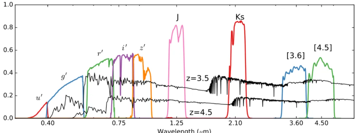
In this study, we use imaging in nine photometric bands spanning the optical to mid-IR in the SHELA Field. The SHELA Field is centered at R.A. = 1h22m00s, declination = +0o₀₀0₀₀00 _{(J2000) and extends approximately±6.5}o _{in R.A. and±1.25}o _{in declination. The} optical bands consist of u0, g0, r0, i0, and z0 from the Dark Energy Camera (DECam) and covers ∼17.8 deg2 of the SHELA footprint (Wold et al. in prep). The field was observed with six pointings with DECam (center coordinates of pointings are listed in Table 1). The mid-IR bands include the 3.6 µm and 4.5 µm from the Infrared Array Camera (IRAC) aboard the Spitzer Space Telescope and covers 24 deg2 (Papovich et al., 2016). In addition, we include near-IR photometry in J and Ks from the February 2017 version of the

VISTA-CFHT Stripe 82 Near-infrared Survey1 _{(VICS82; Geach et al. 2017), which covers ∼85%} of the optical imaging footprint and has 5-σ depths of J = 21.3 mag and Ks = 20.9 mag.

Figure 1 shows the filter transmission curves for the nine photometric bands used overplotted with model high-z galaxy spectra illustrating the wavelength coverage of our dataset.

3.2 DECam Data Reduction and Photometric Calibration

The DECam images were processed by the NOAO Community Pipeline (CP). A detailed description of the Community Pipeline reduction procedure can be found in the DECam Data Handbook on the NOAO website2_{, however, we provide a brief summary of} the procedure here. First, the DECam images were calibrated using calibration exposures

Table 1. DECam Imaging Field Coordinates

Sub-Field R.A. Dec.

ID No. (J2000) (J2000) SHELA-1 1h00m52.8s -0o0003600 SHELA-2 1h₀₇m_02.4s _-0o₀₀0₃₆00 SHELA-3 1h₁₃m_12.0s _-0o₀₀0₃₆00 SHELA-4 1h19m21.6s -0o0003600 SHELA-5 1h₂₅m_31.2s _-0o_g000₃₆00 SHELA-6 1h₃₁m_40.8s _-0o₀₀0₃₆00 0.40 0.75 1.25 2.10 3.60 4.50 Wavelength (µm) 0.0 0.2 0.4 0.6 0.8 1.0 Tra nsm issi on u′ g′ r′ i′ z′

J

Ks

[3.6] [4.5]

z=3.5

z=4.5

Figure 1: The filter transmission curves for the nine photometric bands used in this study (curves are labelled in the figure) and two model star-forming galaxy spectra with redshiftsz = 3.5 andz = 4.5, respectively (black). The model spectra have units of Jy and are arbitrarily scaled. Thez = 3.5 galaxy spectrum falls completely red-ward of the u0 band transmission curve and the z = 4.5 galaxy spectra has almost zero flux falling in the g0 bandpass.

from the observing run. The main calibration steps included an electronic bias calibration, saturation masking, bad pixel masking and interpolation, dark count calibration, linearity correction, and flat-field calibration. Next, the images were astrometrically calibrated with 2MASS reference images. Finally, the images were remapped to a grid where each pixel is a square with a side length of 0.2700. Observations taken on the same night were then co-added. The CP data products for the SHELA field were downloaded from the NOAO Science Archive3. The data products include the co-added images, remapped images, data quality maps (DQMs), exposure time maps (ETMs), and weight maps (WMs). The co-added images from the CP were not intended for scientific use, so we opted to co-add the remapped images. We followed the co-adding procedure of Wold et al. (in prep.), which we summarize here. Using the software package SWARP (Bertin et al., 2002) the sub-images stored in the FITS files of the remapped images were stitched together and background subtracted. The remapped images were combined using a weighted mean procedure optimized for point-sources. The weighting of each image is a function of the seeing, transparency, and sky brightness and is defined by Equation A3 in Gawiser et al. (2006) as

wPS_i = factori scalei×rmsi

!2

, (1)

where scalei is the image transparency (defined as the median brightness of the bright

un-saturated stars after normalizing the brightness measurement of each star by its median brightness across all exposures), rmsi is the root mean square of the fluctuations in

back-ground pixels, and factori is defined as

factori = 1−exp −1.3

FWHM2_stack FWHM2_i

!

, (2)

where FWHMstackis the median FWMH of bright unsaturated stars in an unweighted stacked image and FWHMi is the median FWHM of bright unsaturated stars in each individual

The seeing and transparency measurements were determined using a preliminary source catalog generated for each resampled image using the Source Extractor software package (Bertin & Arnouts, 1996).The seeing in the stacked images are listed in Table 2.

Table 2: DECam Imaging Seeing and Limiting Magnitudes

Band Sub-Field FWHM Depth ID No. (00) (mag) u0 SHELA-1 1.12 25.2 SHELA-2 1.2 25.2 SHELA-3 1.22 25.4 SHELA-4 1.15 25.3 SHELA-5 1.21 25.1 SHELA-6 1.26 25.4 g0 SHELA-1 1.06 24.8 SHELA-2 1.26 24.8 SHELA-3 1.36 25.0 SHELA-4 1.4 24.4 SHELA-5 1.07 24.9 SHELA-6 1.37 24.9 r0 SHELA-1 1.0 24.8 SHELA-2 1.28 24.6 SHELA-3 1.14 24.7 SHELA-4 1.05 24.3 SHELA-5 1.02 24.3 SHELA-6 1.26 24.5 i0 SHELA-1 0.87 24.5 SHELA-2 1.39 23.9 SHELA-3 1.04 24.5 SHELA-4 1.0 22.1 SHELA-5 0.93 23.9 SHELA-6 1.27 24.2 z0 SHELA-1 0.86 23.8 SHELA-2 0.96 23.6 SHELA-3 1.21 23.5 SHELA-4 1.13 23.7 SHELA-5 0.85 23.6 SHELA-6 0.86 23.5

The FWHM values are for the stacked DECam images before PSF match-ing. The magnitudes quoted are the 5-σ limits measured in 1.8900-diameter apertures on the PSF-matched images (see Section 3.3).

After discovering the original WMs from the Community Pipeline had values incon-sistent with the ETM, we created custom rms maps for the co-added images. The initial rms per pixel was defined as the inverse of the square-root of the exposure time. The median of the rms map is scaled to the global pixel-to-pixel rms which is defined as the standard deviation of the fluxes in good-quality, blank sky pixels. Good-quality, blank sky pixels are pixels not included in a source according to our initial Source Extractor catalog (see Section 3.3 for discussion of our source extraction procedure), and have an exposure time greater than 0.9 times the median value.

The DECam imaging data were photometrically calibrated with photometry from the Sloan Digital Sky Survey (SDSS) data release 11 (DR11; Eisenstein et al., 2011) using only F0 stars. F0 stars were used because their spectral energy distribution span all five optical filters while appearing in the sky at a sufficiently high surface density to provide statistically significant numbers in each DECam image. We began by creating a preliminary source catalog for the stacked DECam images using Source Extractor and position matching to the SDSS source catalog. Then we selected F0 stars using SDSS colors by integrating an F0-star model spectrum from the 1993 Kurucz Stellar Atmospheres Atlas (Kurucz, 1979) with each of the five optical SDSS filter curves. For sources in the catalog to be identified as an F0 star, the total color differences, using colors for all adjacent bands, added in quadrature must have been less than 0.35. We then calculate the expected magnitude offset between SDSS and DECam filters for F0 stars, which are as follows: u0: 0.33, g0: 0.02, r0: -0.001, i0: -0.02, and z0: -0.01. The zero-point for each filter was then calculated as

ZPT = median(mAB_SDSS−mDECam −∆moffset), (3) where ∆moffset is the expected magnitude offset between SDSS and DECam filters for F0 stars. After the zero-points were applied to each stacked image, the image pixel values were converted to units of nJy.

3.3 DECam Photometry

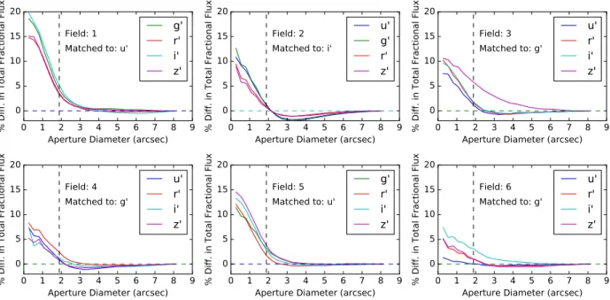
Studying galaxy properties relies on accurate measurements of galaxy colors. One way to obtain accurate colors is to perform fixed-aperture photometry where you measure source fluxes in every band using the same sized aperture. However, since the DECam images where taken in varying seeing conditions they have point spread functions (PSFs) with a range of full width at half maximum (FWHM). To perform fixed-aperture photometry on these images, the PSFs of all the imaging covering a single patch of sky must be adjusted to have a similar PSF size. We divided the DECam imaging into six sub-fields (each defined as roughly one DECam pointing). For each sub-field, we enlarged the PSFs of the stacked images to match the PSF of the stacked image with the largest PSF in that sub-field. For example, in sub-field SHELA-1 we matched the PSFs of theg0,r0,i0, andz0stacked images to the PSF of theu0 band. To enlarge the PSFs we adopted the procedure of Finkelstein et al. (2015) who used the IDL deconv tool Lucy-Richardson deconvolution routine. This routine takes as inputs two PSFs (the desired larger PSF and the starting smaller PSF) and the number of iterations to run and outputs a convolution kernel. The input image PSFs were produced by median combining the 100 brightest stars (sources with stellar classifications in SDSS DR11) in each image. Before combining, the stars were over-sampled by a factor of 10, re-centered, and then binned by ten to ensure the star centroids aligned. We ran the deconvolution routine with an increasing number of iterations until the PSF of the convolved image (again measured from stacking stars) had a flux within a 7-pixel (1.8900) diameter aperture matched to that of the PSF of the target image to within 5%. The total fluxes were measured in 30-pixel (8.100) diameter circular apertures. In Figure 2 we show the results of PSF-matching in each sub-field by displaying a comparison of the enlarged PSFs to the largest PSF as a percent difference.

Due to variations in intrinsic galaxy colors and variable image depth and sky coverage, some galaxies will not appear in all bands. To get photometric measurements of all sources in every DECam image we combined the information in the five optical band images into a single detection image. We followed the procedure of Szalay et al. (1999) and summed the

0 1 2 3 4 5 6 7 8 9 Aperture Diameter (arcsec) 0 5 10 15 20 % Dif f. i n T ota l F rac tio na l F lux Field: 1 Matched to: u'

g'

r'

i'

z'

0 1 2 3 4 5 6 7 8 9 Aperture Diameter (arcsec) 0 5 10 15 20 % Dif f. i n T ota l F rac tio na l F lux Field: 2 Matched to: i'

u'

g'

r'

z'

0 1 2 3 4 5 6 7 8 9 Aperture Diameter (arcsec) 0 5 10 15 20 % Dif f. i n T ota l F rac tio na l F lux Field: 3 Matched to: g'

u'

r'

i'

z'

0 1 2 3 4 5 6 7 8 9 Aperture Diameter (arcsec) 0 5 10 15 20 % Dif f. i n T ota l F rac tio na l F lux Field: 4 Matched to: g'

u'

r'

i'

z'

0 1 2 3 4 5 6 7 8 9 Aperture Diameter (arcsec) 0 5 10 15 20 % Dif f. i n T ota l F rac tio na l F lux Field: 5 Matched to: u'

g'

r'

i'

z'

0 1 2 3 4 5 6 7 8 9 Aperture Diameter (arcsec) 0 5 10 15 20 % Dif f. i n T ota l F rac tio na l F lux Field: 6 Matched to: g'

u'

r'

i'

z'

Figure 2: The results of PSF-matching the DECam images. Each panel shows the percent difference between the enlarged PSFs and the largest PSF per SHELA sub-field. The colored lines correspond to the four bands listed in each panel’s legend. The vertical dashed line denotes 1.89” which is the aperture diameter at which we compared PSFs during the PSF-matching procedure (see Section 3.3 for details). The horizontal dashed line was placed to zero to guide the eye. This figure illustrates that all bands in all sub-fields have PSFs that collect the same fraction of light as their respective largest PSF to within 5% except for the z0 band in sub-field 3 which matches to about 6%.

square of the signal-to-noise ratio in each band pixel-by-pixel as follows: Di = s XF_band2 _,i σ2 band,i , (4)

whereDi is the detection imageith pixel value,Fband,i is theith pixel flux in the band image,

and σband,i is the rms at thatith pixel pulled from the the band rms image. A weight image

associated with this detection image was created where pixels associated with detection map pixels with data in at least one band have a value of unity and pixels associated with detection map pixels without data have a value of zero.

Photometry was measured on the PSF-matched images using the Source Extractor software (v2.19.5, Bertin & Arnouts, 1996). Catalogs were created for each of the six SHELA sub-fields with Source Extractor in two image mode using the detection image described above, and cycling through the five DECam bands as the measurement image. In the final source catalog, we maximized the detection of faint sources while minimizing false detections by optimizing the combination of the SExtractor parameters DETECT THRESH and DETECT MINAREA. We did this by running SExtractor with an array of combinations of DETECT THRESH and DETECT MINAREA and chose the combination of 1.6 and 3, respectively, which detected all sources that appeared real by visual inspection and included the fewest false positive detections from random noise fluctuations.

We measure source colors in 1.8900 diameter circular apertures (which corresponds to an enclosed flux fraction of 59-75% for unresolved sources in our sub-fields). To obtain the total flux, we derived an aperture correction defined as the flux in a 1.8900 diameter aperture divided by the flux in a Kron aperture (i.e., FLUX AUTO), using the default Kron aperture parameters of PHOT AUTOPARAM= 2.5, 3.5, which has been shown to calculate the total flux to within∼5% (Finkelstein et al., 2015). This correction was derived in the r0-band on a per-object basis to account for different source sizes and ellipticities and was applied to the fluxes in the other DECam bands per sub-field. In areas where the sub-fields overlapped, sources with positions that matched to within 1.200 in neighboring sub-field catalogs had their fluxes mean-combined after being weighted by the inverse square of their uncertainties (see Section 3.4). The DECam source fluxes were corrected for Galactic extinction using the

color excess E(B-V) measurements by Schlafly & Finkbeiner (2011). We obtained E(B-V) values using the Galactic Dust Reddening and Extinction application on the NASA/IPAC Infrared Science Archive (IRAS) website4_{. We queried IRAS for E(B-V) values (the mean} value within a 5 radius) for a grid of points across the SHELA field with 4 spacing and assigned each source the E(B-V) value from the closest grid point. The Cardelli et al. (1989) Milky Way reddening curve parameterized byRV = 3.1 was used to derive the corrections at

each band’s central wavelength. We compared the extinction-corrected DECam photometry to SDSS DR14 per sub-field and band and found agreement for point sources to better than δm <0.05−0.2 mag in terms of scatter.

3.4 DECam Photometric Errors

We estimated photometric uncertainties in the DECam images by estimating the image noise in apertures as a function of pixels per aperture, N, following the procedure described in Section 2 of Papovich et al. (2016). There are two limiting cases for the un-certainty in apertures with N pixels, σN. If pixel errors are completely uncorrelated, the

aperture uncertainty scales as the square root of the number of pixels, σN = σ1 ×

√

N, where σ1 is the standard deviation of sky background pixels. If pixel errors are completely correlated then σN =σ1×N (Quadri et al., 2006). Thus, the aperture uncertainty will scale as Nβ _{with 0.5< β <1.}

To estimate the aperture noise as a function of N pixels, we measured the sky counts in 80,000 randomly placed apertures ranging in diameter from 000.27 to 800.1 across each stacked DECam image. We required apertures to fall in regions of the background sky, which we define as the region where the exposure time map has the value of the at least the median exposure time (ensuring>50% of each image was considered), excluding detected sources and pixels flagged in the DQM. We also required the apertures do not overlap with each other. We then estimatedσN for each aperture with N pixels by computing the standard deviation

(Beers et al., 1990). We calculated σ1 by computing σnmad for all pixels in the background sky as defined above. Figure 3 shows an example of the measured flux uncertainty in a given aperture, σN, as a function of the square root of the number of pixels in each aperture, N,

for the five DECam bands in the sub-field SHELA-1.

Following Papovich et al., 2016 we fit a parameterized function to the noise in an aperture of N pixels, σN, as,

σN =σ1(αNβ +γNδ), (5)

where σ1 is the pixel-to-pixel standard deviation in the sky background, and α, β, γ, and δ are free parameters. The best-fitting parameters in Equation 5 for the combined DECam images are listed in Table 3. While the second term was intended to aid in fitting the data at large N values, in actuality the second term contributed significantly at all N values resulting in β ≈0.9-1. Nevertheless our functional fits reproduce the data well as can be seen, for example, in Figure 3. To estimate how correlated the pixel-to-pixel noise is, we fit σN with only the first term in Equation 5 and found typical values of β ≈ 0.65-0.70

suggesting slightly correlated pixel-to-pixel noise.

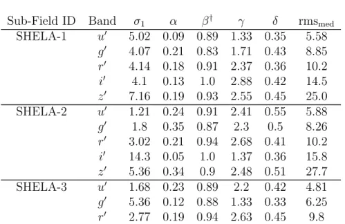
Table 3: Fit Parameters for Background Fluctuations as Function of Aper-ture Size Using Eq.(5)

Sub-Field ID Band σ1 α β† γ δ rmsmed SHELA-1 u0 5.02 0.09 0.89 1.33 0.35 5.58 g0 4.07 0.21 0.83 1.71 0.43 8.85 r0 4.14 0.18 0.91 2.37 0.36 10.2 i0 4.1 0.13 1.0 2.88 0.42 14.5 z0 7.16 0.19 0.93 2.55 0.45 25.0 SHELA-2 u0 1.21 0.24 0.91 2.41 0.55 5.88 g0 1.8 0.35 0.87 2.3 0.5 8.26 r0 3.02 0.21 0.94 2.68 0.41 10.2 i0 14.3 0.05 1.0 1.37 0.36 15.8 z0 5.36 0.34 0.9 2.48 0.51 27.7 SHELA-3 u0 1.68 0.23 0.89 2.2 0.42 4.81 g0 5.36 0.12 0.88 1.33 0.33 6.25 r0 2.77 0.19 0.94 2.63 0.45 9.8

†_{Typical values of β ≈ 0.65-0.70 when using a two parameter fit (i.e. with} onlyα and β) suggest slightly correlated noise between pixels.

Table 3 cont.

Sub-Field ID Band σ1 α β† γ δ rmsmed

i0 3.06 0.32 0.92 3.07 0.38 12.6 z0 11.0 0.15 0.91 1.95 0.41 24.1 SHELA-4 u0 1.08 0.26 0.95 2.54 0.49 4.64 g0 7.36 0.13 0.85 1.24 0.34 8.31 r0 2.86 0.25 0.91 2.44 0.51 12.1 i0 24.9 1.42 0.6 1.27 0.6 63.5 z0 5.48 0.26 0.93 2.79 0.45 22.6 SHELA-5 u0 5.25 0.11 0.87 1.25 0.33 5.8 g0 3.11 0.23 0.87 1.92 0.43 7.86 r0 4.78 0.38 0.81 2.02 0.46 15.8 i0 5.53 0.33 0.85 2.32 0.46 21.9 z0 6.86 0.23 0.92 2.53 0.49 28.0 SHELA-6 u0 1.66 0.15 0.95 2.38 0.42 4.6 g0 6.15 0.12 0.86 1.27 0.32 6.8 r0 4.81 0.21 0.87 2.09 0.4 12.1 i0 6.87 0.14 0.93 2.14 0.37 14.7 z0 6.09 0.51 0.82 2.13 0.53 32.8 †

Typical values of β ≈ 0.65-0.70 when using a two parameter fit (i.e. with onlyα and β) suggest slightly correlated noise between pixels.

The photometric errors estimated by Equation 5 were scaled to apply to flux mea-surements outside the region with the median exposure time. The flux uncertainty for the i-th source in bandb in the sub-field f is calculated as

σ_i,f,b2 =σ2_N,f,b rmsi,f,b rmsmed,f,b

!2

, (6)

whereσN,f,b is given by Equation 5 for each band and sub-field, rmsi,f,bis the value of the rms

map at the central pixel location of thei-th source in each band and sub-field, and rmsmed,f,b

is the median value of the rms map in each band and sub-field. The photometric error estimates exclude Poisson photon errors, which we estimate to contribute <5% uncertainty to the optical fluxes of our high-z candidates.

0 5 10 15 20 25 N 0 200 400 600 800 1000 σN ( nJ y) β = 1 z′ i′ r′ g′ u′ β = 0.5

Figure 3: Background noise fluctuations, σN, in an aperture of N pixels

plotted as a function of the square root of the number of pixels for the five DECam band images in sub-field SHELA-1. The colored dotted lines are the measured aperture fluxes and the solid lines are fits to the data. See legend insert for color coding information. The dot-dashed line shows the relation assuming uncorrelated pixels, σN ∼

√

N . The dashed line shows the relation assuming perfectly correlated pixels (σN ∼ N; Quadri et al.,

the apertures were scaled by the same amount to determine the total flux uncertainties, so that the S/N for the total flux is the same as for the aperture flux.

3.5 IRAC data reduction and photometry

As discussed below, we wish to enhance the validity of our z = 4 galaxy sample by including IRAC photometry in our galaxy sample selection. While we could allow this by position-matching the published Spitzer/IRAC catalog from Papovich et al. (2016) to our DECam catalog, this is not optimal for two reasons. First, the Papovich et al. (2016) catalog is IRAC-detected, and so only includes sources with significant IRAC flux, while for our purposes, even a non-detection in IRAC can be useful for calculating a photometric redshift. Second, this catalog uses apertures defined on the positions and shapes of the IRAC sources, while the larger PSF of the IRAC data results in significant blending, which is a larger issue at fainter magnitudes, where we expect to find the bulk of our sources of interest. For these reasons, we applied the Tractor image modeling code (Lang et al., 2016a,b) to perform “forced photometry”, which employs prior measurements of source positions and surface brightness profiles from a high-resolution band to model and fit the fluxes of the source in the remaining bands, splitting the flux in overlapping objects into their respective sources. We specifically used the Tractor to optimize the likelihood for the photometric properties of DECam sources in each of IRAC 3.6 and 4.5µm bands given initial information on the source and image parameters. The input image parameters of IRAC 3.6 and 4.5µm images included a noise mode, a point spread function (PSF) model, image astrometric information (WCS), and calibration information (the “sky noise” or rms of the image background). The input source parameters included the DECam source positions, brightness, and surface brightness profile shapes. The Tractor proceeds by rendering a model of a galaxy or a point source convolved with the image PSF model at each IRAC band and then performs a linear least-square fit for source fluxes such that the sum of source fluxes is closest to the actual image pixels, with respect to the noise model. We describe how we use the Tractor to perform forced photometry on IRAC images in detail below.

model of each source. We use the fluxes and surface brightness profile shape parameters measured in our DECam detection image because the image combines the information of all sources in the five optical band images (as described in Section 3.3). Second, we use one-component circular Gaussian to model the PSF. During the modeling of each source, we allow Tractor to optimize the Gaussian σ value, in addition to optimize a source flux. We find that the median of the optimized Gaussian σ is 000.80 (equivalent to a full-width at half maximum of 100.88) for both IRAC 3.6 and 4.5 µm images, consistent with those measured from an empirical point response function for the 3.6µm and 4.5µm image (FWHM of 100.97, see Papovich 2016, Section 3.4).

In practice, we extracted an IRAC image cutout of each source in the input DECam catalog. We selected the cutout size of 1600 ×1600. This cutout size represents a trade-off between minimizing computational costs related to larger cutout sizes and ensuring that the sources lie well within the cutout extent. The sources of interest within cutout are modeled as either unresolved (i.e., a point source) or resolved based on the DECam detection image. We considered a source to be resolved if an estimated radius r > 000.1. We define the radius as, rsource = a×

p

b/a, where a is a semi-major axis and b/a is an axis ratio. We perform the photometry for resolved sources using a deVaucouleurs profile (equivalent to S´ersic profile with n=4) with shape parameters (semi-major axis, position angle, and axis ratio) measured using our DECam detection image. We have also performed the photometry using an exponential profile (equivalent to S´ersic profile with n=1), but we do not find any significant difference between the IRAC flux measurements for the two galaxy profiles. Therefore, we adopt a deVaucouleurs profile to model all resolved sources. The Tractor simultaneously modeled and optimized the sources of interest and neighboring sources within the cutout. Finally, the Tractor provided the measurement IRAC flux of each DECam source with the lowest reduced chi-squared value. We validated the Tractor-based IRAC fluxes by comparing the fluxes of isolated sources (no neighbors within 300) to the published

Spitzer/IRAC catalog from Papovich et al. (2016). For both bands, we found good agreement

with a bias offset ofδm < 0.05 mag and a scatter of <0.11 mag down tom= 20.5 mag and a bias offset of δm < 0.13 mag and a scatter of <0.26 down to m= 22 mag.

4

Sample Selection

4.1 Photometric Redshifts and Selection Criteria

We selected our sample of high-redshift galaxies using a selection procedure that relies on photometric redshift (zphot) fitting, which leverages the combined information in all photometric bands used. We obtained zphot’s andzphot probability distribution functions (PDFs) from the EAZY software package (Brammer et al., 2008). For this analysis, we use the “z a” redshift column from EAZY which is produced by minimizing the χ2 in the all-template linear combination mode. We also tried the “z peak” column and our resulting luminosity function did not change significantly. EAZY assumes the intergalactic medium (IGM) prescription of Madau (1995). We did not use any magnitude priors based on galaxy luminosity functions when running EAZY as the existing uncertainties in the bright-end would bias our results (effectively assuming a flat prior). We then applied a number of selection criteria using the zphot PDFs from EAZY following the procedure of Finkelstein et al. (2015), which we summarize here, to construct a z ≈ 4 galaxy sample. First, we required a source to have a signal-to-noise ratio of greater than 3.5 in the two photometric bands (r0 and i0 bands) that probe the UV continuum of our galaxy sample, which has been shown to limit contamination by noise to negligible amounts by Finkelstein et al. (2015). Next we required the integral of each source’s zphot PDF for z > 2.5 to be greater than 0.8 and the integral of the zphot PDF from z = 3.5-4.5 to be greater than the integral of the zphot PDF in all other ∆z = 1 bins centered on integer-valued redshifts. Finally, we required a source to have no photometric flags on its u0, g0, r0, and i0 flux measurements in our photometric catalog. These four bands are crucial for probing both sides of the Lyman break of galaxies in the redshift range of interest. Photometric flags indicate saturated pixels, transient sources, or bad pixels as defined by the CP (see section 3.2).

Initially, we required sources to pass this zphot selection procedure when only the DECam and IRAC bands were used. After inspecting candidates from this selection and finding low-z contaminants (see Section 4.2) we moved to include the VISTA J and K

as described in the following section, however, a new class of contaminant appeared in the candidate sample due to erroneous VISTA photometry for some sources. To overcome this we required a source to pass thezphot selection process with and without including the VISTAJ and K photometry. This doublezphot selection process resulted in an initial sample of 4,364 high-z objects. Next, we performed an investigation into possible contamination, which resulted in additional selection criteria and a refined sample.

4.2 Identifying Contamination

Photometric studies of high-z objects can be contaminated by galactic stars and low-z galaxies whose 4000 ˚A break can mimic the Lyman-α break of high-z galaxies. The inclusion of IRAC photometry is crucially important for removing galactic stars from our sample as galactic stars have optical colors very similar to z = 4 objects (Figure 4). While inspecting the photometry and best-fitting SED templates to confirm our fits were robust and our high-z galaxy candidates were convincing we found evidence of contamination in our preliminary photometrically selected sample. We explored ways of identifying and removing the contamination including cross-matching our sample with proper motion catalogs, SDSS spectroscopy, and X-ray catalogs. Additionally, we implemented machine learning methods.

4.2.1 Cross-matching with NOMAD and SDSS

While inspecting the photometry of our preliminary sample derived before the inclu-sion of the VISTA data we found a fraction of candidates had redr0−i0 colors and excesses in the i0 and z0 bands with respect to the best fitting z ∼4 template. We investigated whether these objects had low redshift origins by cross-matching our sample with the Naval Ob-servatory Merged Astrometric Dataset (NOMAD) proper motion catalog (Zacharias et al., 2004) and the SDSS spectral catalog (DR13; Albareti et al. 2017). The cross-matching with NOMAD resulted in the identification of 16 objects with proper motion measurements, 6 of which were large in magnitude suggesting that these sources were stellar contaminants. Cross-matching with SDSS spectra resulted in the identification of 23 z ∼ 4 QSOs, two low

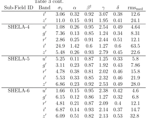
−0.5 0.0 0.5 1.0 1.5 2.0 2.5 r′_{− i}′ [mag] −0.5 0.0 0.5 1.0 1.5 2.0 2.5 3.0 g ′− r ′ [m ag ] AGN (3. 2 ≤ zspec< 3. 5) AGN (4. 5 ≤ zspec< 4. 8) Final Candidates (mi′< 22) Candidates omitted b colors (mi′< 22) Stars (S/Ni′> 100) AGN (3. 5 ≤ zspec< 4. 5) −0.5 0.0 0.5 1.0 1.5 2.0 2.5 r′_{− i}′ [mag] −2 −1 0 1 2 i ′− [3 .6] [m ag ] AGN (3. 2 ≤ zspec< 3. 5) AGN (4. 5 ≤ zspec< 4. 8) Final Candidates (mi′< 22) Candidates omitted b colors (mi′< 22) Stars (S/Ni′> 100) AGN (3. 5 ≤ zspec< 4. 5)

Figure 4: Left: Color-color plot showing DECam g0 −r0 vs r0 −i0. Blue points correspond to bright (S/Ni > 100) sources classified as stars within

SDSS DR14. Sources spectroscopic identified as QSO within SDSS DR13 at 3.2 ≤ z < 3.5, 3.5 ≤ z < 4.5, and 4.5 ≤ z < 4.8 are orange circles, black “x”s, and green circles, respectively. Bright candidate objects from our study are shown as squares (see legend insert for color coding). Right: Color-color plot showing i0 −[3.6] vs r0 −i0. The r0 −i < 1.0 and the i0 −[3.6] > −0.2 color selection criteria are denoted as the vertical dashed line and the horizontal dashed line, respectively. No candidates are hidden by the legend inserts. These plots illustrate how the inclusion of IRAC photometry breaks the optical color degeneracy ofz = 4 sources and galactic stars. In the left panel where only optical colors are used the z ∼ 4 AGNs share the parameter space of galactic stars, while in the right panel where one color includes the [3.6] IRAC band there is a larger separation.

mass stars, and one low-z galaxy in our sample. All of the stellar objects and the low-z galaxy had redr0−i0 colors confirming our suspicion that a fraction of our sample had low-z origins. We removed from our candidate sample the 6 objects with proper motions above 50 mas/yr in NOMAD. We chose the threshold 50 mas/yr because some SDSS QSOs are reported to have small nonzero proper motions in the NOMAD catalog. After inclusion of the VISTA J and K photometry, 5 of the 6 rejected objects became best-fit by a low-z solution and therefore were rejected by our selection process automatically. Results like this suggested the inclusion of the VISTA data improved the fidelity of our sample.

4.2.2 Cross-matching with X-ray catalog Stripe 82X

In principle, AGNs can be distinguished from UV-bright star-forming galaxies at high z by their X-ray emission as AGNs dominate X-ray number counts down to FX =

1×10−17erg cm−2 s−1in 0.5-2 keVChandra imaging (Lehmer et al., 2012). In fact, Giallongo et al. (2015) found 22 AGN candidates at z > 4 by measuring fluxes in deep 0.5-2 keV

Chandra imaging at the positions of their optically-selected candidates. They required AGN

candidates to have an X-ray detection of FX > 1.5×10−17 erg cm−2 s−1. We attempted

to identify AGNs in our candidate sample by position matching with the 31 deg2 _Stripe 82X X-ray catalog (LaMassa et al., 2016). Unfortunately, the flux limit at 0.5-2 keV was 8.7×10−16 _{erg cm}−2 _s−1_{, shallower than the detection threshold used by Giallongo et al.} (2015). Cross-matching the Stripe 82X X-ray Catalog with our candidate sample resulted in 8 matches within 700 or the matching radius used by LaMassa et al. (2016) to match the Stripe 82X X-ray Catalog with ancillary data. Two of the X-ray-matched sources (mi0 ≈19) are SDSS AGNs, although one has two extended objects within the 700 matching radius, drawing into question the likelihood of the match. Another X-ray-matched source (mi0 ≈22) is a very red object (r0 −i0 = −0.9 and i0 −[3.6] =3.4) without SDSS spectroscopy. The remaining five X-ray-matched sources are fainter (mi0 ≈24) and without SDSS spectroscopy, and two have large separations (> 600) with their X-ray counterpart. All 8 X-ray-matched sources satisfied each of our selection criteria and made it into our final sample.

4.2.3 Insights from machine learning

To further understand and minimize the contamination in our preliminary sample we utilized two machine learning algorithms: a decision tree algorithm and a random forest algorithm. First, we tried the decision tree algorithm from the sci-kit learn Python package (Pedregosa et al., 2011). Executing the decision tree algorithm involved creating a training set by classifying (via visual inspection) the 300 brightest objects as one of five types: 1. obviously high-z galaxy or high-z AGN, 2. obviously low-z galaxy, 3. indistinguishable between high-z or low-z object, 4. SDSS spectroscopically identified QSO, 5. spurious source. The classification was driven by a combination of the shape of the optical SED, the χ2 of the best fitting high-z (z ∼ 4) galaxy template, the difference in χ2 between the best fitting high-z galaxy template and the best fitting low-z galaxy template, SDSS spectral classification, and proper motion measurements. The obviously high-z objects and the SDSS QSOs had roughly flat rest-UV spectral slopes (i.e., thei0,r0, andz0 fluxes were comparable) while the obviously low-z objects had a clear spectral peak between the optical and mid-IR, specifically the r0 −i0 and i0 −z0 colors were quite red while the z0 −[3.6] was blue. We then selected three data ”features” or measurements for the decision tree to choose from to predict the classifications of the training set: 1. The χ2 _{of the best fitting high-z galaxy} template, 2. The r0−i0 color, and 3. The signal-to-noise ratio in the u0 band. We include this signal-to-noise ratio because most obviously high-z sources had a signal-to-noise ratio of less than 3 (as they should, as this filter is completely blue-ward of the Lyman break for the target redshift range) while the obviously low-z source did not. We restricted the training set to include only the obviously high-z objects (including SDSS classified QSOs) and obviously low-z objects.

To evaluate the decision tree performance we assigned 34% of the training set to a test set and left the test set out of the first round of training. The first round of training was validated using three-fold cross-validation with a score of 94+/-2%. Three-fold cross validation verifies the model is not over-fitting or overly dependent on a small randomly

combination of two sub-samples while validating on the remaining sub-sample, and then averaging the validation scores of all the combinations. A validation score of 100% indicates each sub-sample combination trained a model that successfully predicted the classifications of every object in the remaining sub-sample. After validation, we applied the model to the test set and achieved a test score of 91%. We then incorporated the test set into the training set and retrained the model. This second round of training had a 3-fold cross validation score of 94 ± 5%. The algorithm determined that classification of the training set could be predicted at 92% accuracy using the r0 −i0 color and the χ2 _{only, where obviously high-z} objects have r0−i0 < 0.555 and χ2 _<70.6.

After performing the decision tree machine learning we tried the random forest algo-rithm by using the scikit-learn routine RandomForestClassifier (Pedregosa et al., 2011). The random forest algorithm uses the combined information of all the features of our dataset instead of using only the three well-motivated features that we provided the decision tree al-gorithm. The random forest algorithm fits a number of decision tree classifiers on a randomly drawn and bootstrapped subset of the data using a randomly drawn subset of the dataset features. The decision tree classifiers are averaged to maximize accuracy and control over-fitting. To provide the best classifications to the algorithm we re-inspected the photometry and the besting-fitting EAZY template SEDs of the brightest 311 objects (mi0 <22.9) and classified by eye each with a probability of being at high z, at low z, and a spurious source. We also inspected the best-fitting EAZY template at the redshift of the second highest peak in the redshift PDF, which was usually betweenz = 0.1−0.5. The features we provided the algorithm included all colors using the DECam and IRAC photometric bands, the χ2 value of the best-fitting EAZY template, and the u-band S/N ratio. We ran the random forest algorithm using 1000 estimators (or decision trees) with a max depth of two and balanced class weights. While the classification accuracy of the random forest was only marginally better than the decision tree, we were able to determine the relative importance of the fea-tures within the random forest. The most important feature was the i0 −[3.6] color, which was consistent with our prior observations of the low-z contaminants having blue z0 −[3.6] while the SDSS classified AGNs had flat or redz0−[3.6]. We compared the predictive power

of the random forest algorithm to that of a simple i0 −[3.6] color cut–where high-z candi-dates were required to have an i0 −[3.6]> −0.2–and found the simple color cut to be just as predictive. We, therefore, elected to adopt the simple i0−[3.6] color cut as an additional step in our selection process. After we applied this cut our high-z object sample consisted of 3,833 objects. We then inspected the brightest 3,200 brightest candidates (mi0 < 24.0) and removed 61 spurious sources cutting our candidate sample to 3,772 objects. The final step in our candidate selection process was an r0 −i0 color cut, which was a result of the contamination test described in the following subsection.

4.3 Estimating Contamination Using Dimmed Real Sources

We estimated the contamination in our high-z galaxy sample by simulating faint and low-S/N low-z interloper galaxies following a procedure used by Finkelstein et al. (2015). We did this by selecting a sample of bright low-z sources from our catalog, dimming and perturbing their fluxes, and assigned the appropriate uncertainties to their dimmed fluxes. This empirical test assumes that bright low-z galaxies have the same colors as the faint lower-z galaxies. The sources we dimmed all had mr0 = 14.3 - 18 mag, brighter than our brightest z =3.5-4.5 candidate source, a best-fitting zphot of 0.1 < zphot < 0.6, and no photometric flags in any optical band (see section 3.2 for definition of photometric flag). We reduced the source fluxes randomly to create a flat distribution of dimmed r0-band mag spanning the range of our candidate high-z galaxies (mr0 = 18-26). We assigned flux uncertainties to the dimmed fluxes by randomly drawing from the flux uncertainties of our candidate high-z galaxy sample. We then perturbed the dimmed fluxes simulating photometric scatter by drawing flux perturbations from a Gaussian distribution with a standard deviation equal to the assigned flux uncertainties. Since the VISTA J and K photometry from the VICS82 Survey covered∼85% of the total SHELA survey area,∼15% of our high-z galaxy candidates do not have flux measurements in the VISTA bands. We incorporated this property of our catalog into the mock catalog by randomly omitting dimmed J and K fluxes at the same rate as the fraction of missingJ and K fluxes in our final sample for a given m bin.

our selection criteria in an identical manner as our real catalog. We found 30,594 artificially dimmed sources satisfied our zphot = 4 selection criteria. We inspected the undimmed and unperturbed properties of these sources and found a range ofr0−i0 colors (0< r0−i0 <1.4), and the objects with the reddest r0−i0 colors contaminated at the highest rate. We defined the contamination rate in the i-th r0 −i0 color bin as

Ri =

Ndimmed,selected,i Ndimmed,i

, (7)

where Ndimmed,selected,i is the number of dimmed sources satisfying our zphot = 4 criteria in thei-th r0−i0 color bin andNdimmed,i is the total number of dimmed sources in thei-thr0−i0

color bin. We created seven r0 −i0 color bins spanning the range of r0−i0 colors recovered (0< r0 −i0 <1.4) with each bin having width=0.2 mag. The contamination fraction, F, in our high-z galaxy sample was defined as

F = P i Ri×Ntotal,i (1−Ri) Nz , (8)

where Ri is the contamination rate defined by Equation 7, Ntotal,i is the total number of

sources in our object catalog in the i-th r0 −i0 color bin with 0.1 < zphot < 0.6 and Nz is

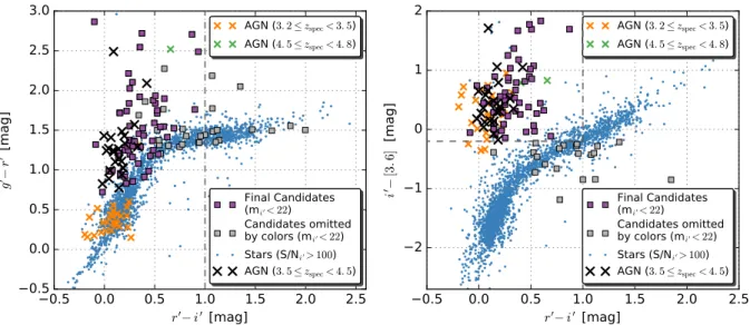
the number of high-z candidates in our final sample in a given redshift bin. We calculated F as a function of mr0 and m_i0 and found contamination fractions of between 0-20% gen-erally increasing as a function of magnitude and not exceeding 25% in any magnitude bin above our 50%-completeness limit (mi0 > 23.5). We learned we can improve our fidelity by implementing a r0−i0 <1.0 color cut, given that the objects with the reddest r0−i0 colors contaminated at the highest rate. We then re-ran our contamination simulation with our final set of selection criteria and found improvement by a few percentage points in two of our brighter magnitude bins (mi0 = 18.75, 20.5) and, again, contamination fractions of between 0-20% generally increasing as a function of magnitude and not exceeding 25% in any mag-nitude bin brighter than our 50%-completeness limit as shown in Figure 5. The addition of the r0−i0 <1.0 color cut reduced our high-z candidate sample size from 3,772 to the final size of 3,740 with a median zphot of 3.8. The measured i0-band magnitude and the redshift

18 19 20 21 22 23 24 25 Apparent Magnitude (mag)

0.0 0.2 0.4 0.6 0.8 1.0 Co nt am ina tio n Fr ac tio n, F P(z) only P(z) + i0₋[3.6] P(z) + i0₋[3.6] + _r0_−i0 50%-Completeness Limit

Figure 5: The results of our contamination simulations estimating the con-tamination fraction using dimmed real sources, showing the concon-tamination fraction, F, as a function of mi0 (solid and dashed colored lines) and m_r0 (dotted colored lines). The color of the lines represent the selection criteria applied before F was calculated: blue for F after only thezphot PDF

selec-tion cuts, purple forF after the zphot PDF selection and the i0−[3.6] color

cuts, and orange forF after the zphot PDF selection, thei0−[3.6] color, and

the r0−i0 color cuts. The error bars indicate the standard deviation of the mean from subdividing our 4.8 million simulated sources into 20 subsamples. The final contamination fraction was found to be between 0-20% generally increasing as a function of magnitude and not exceeding 25% in any magni-tude bin brighter than our 50%-completeness limit mi0 ≈ 23.5 (black solid line).

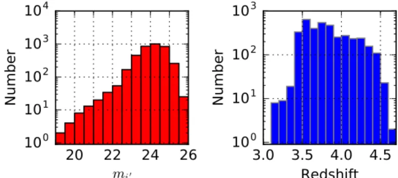
distribution of our final sample is shown in Figure 6. A summary of our sample selection criteria is listed in Table 4. Bright (mi0 < 22) candidates are plotted in Figure 5 showing the distinct color parameter space they occupy (along with SDSS spectroscopically classified AGNs) compared to the parameter space occupied by SDSS spectroscopically classified stars in the SHELA field.

4.4 Completeness Simulations

ef-20 22 24 26

m

i′

10

0

10

1

10

2

10

3

10

4

Nu

mb

er

3.0 3.5 4.0 4.5

Redshift

10

0

10

1

10

2

10

3

Nu

mb

er

Figure 6: The i0-band magnitude distribution (left) and the photometric redshift distribution (right) of our final sample ofz ≈4 candidates. Photo-metric redshifts are the redshifts whereχ2 is minimized for the all-template linear combination mode from the EAZY software (z a). We have found high-zsources over a wide range of brightnesses and across the entirez =3.5-4.5 range.

Table 4. Summary ofz = 4 Sample Selection Criteria

Criterion Section Reference

S/Nr0 >3.5 (4.1)

S/Ni0 >3.5 (4.1)

R∞

2.5PDF(z) dz >0.8 (4.1)

R4.5

3.5 PDF(z) dz >All other ∆z = 1 bins (4.1) i0−[3.6]>−0.2 (4.2.3)

survey incompleteness due to image depth and selection effects. To quantify the survey in-completeness we simulated a diverse population of high-zgalaxies with assigned photometric properties and uncertainties consistent with our source catalog and measured the fraction of simulated sources that satisfied our high-z galaxy selection criteria as a function of the absolute magnitude and redshift.

The simulated mock galaxies were given properties drawn from distributions in red-shift and dust attenuation (e.g., E[B-V]) while the ages and metallicities were fixed at 0.2 Gyr and solar (Z = Z), respectively. Because the fraction of recovered galaxies per redshift bin is independent of the number of simulated galaxies per redshift bin as long as low-number statistics are avoided, the redshift distribution was defined to be flat from 2< z <6, and the E(B-V) distribution was defined to be log-normal spanning 0< E(B-V)<1 and peaking at 0.2. Mock SEDs were then generated for each galaxy using pythonFSPS5 _{(Foreman-Mackey} et al. 2014), a python package that calls the Flexible Stellar Population Synthesis Fortran library (Conroy et al., 2009; Conroy & Gunn, 2010). We then integrated each galaxy SED through our nine filters (DECam u0, g0, r0, i0, and z0; VISTA J and K; and IRAC 3.6 µm and 4.5 µm). Each set of mock photometry was then scaled to have an r-band apparent magnitude within a log-normal distribution spanning 18 < mr0 < 27. This distribution en-sured we were simulating the most galaxies at the fainter magnitudes where we expected to be incomplete and fewer at bright magnitudes where we expected to be very complete. Flux uncertainties and missing VISTA fluxes were assigned in the same way as during the contamination test in Section 4.3. Mock galaxies were not assigned photometric flags. This likely results in an incompleteness of only a couple percent as the fraction of all sources affected by flags is small. All sources with a signal-to-noise ratio of greater than 3.5 in any one band, are flagged in another band less than 2% of the time on average (never exceeding 4%). In addition all images have ∼0.5% of all pixels flagged on average (never exceeding 2%).

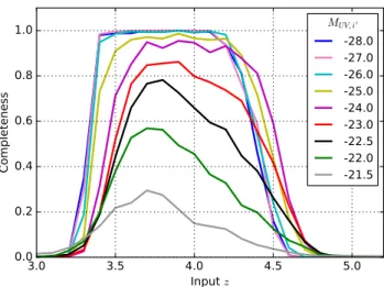
generate zphot PDFs and our high-z galaxy selection was applied. The completeness was defined as the number of mock galaxies recovered divided by the number of input mock galaxies, as a function of input absolute magnitude and redshift. Figure 7 shows the results of our simulation. We define the 50%-completeness limit as the absolute magnitude where the area under the curve falls to less than 50% the areas under the average of theMU V,i0 =−25 toMU V,i0 =−28 curves, which we find to be at M_{U V,i}0 =−22 (m= 24 for z = 4).

3.0 3.5 4.0 4.5 5.0 Input z 0.0 0.2 0.4 0.6 0.8 1.0 Co mp let en ess MUV, i′ -28.0 -27.0 -26.0 -25.0 -24.0 -23.0 -22.5 -22.0 -21.5

Figure 7: The results of our completeness simulations, showing the fraction of simulated sources recovered as a function of input redshift. Each colored line is for the corresponding 0.5 magnitude bin according to the legend. We define the 50%-completeness limit as the absolute magnitude curve with an integral value of less than 50% the area under the average of theM1450 =−25 toM1450 =−28 curves. We find the 50%-completeness to beM1450 =−22.0.

5

Results

5.1 The Rest-Frame UV z=4 Luminosity Function

We utilize the effective volume method to correct for incompleteness in deriving our luminosity function. The effective volume (Vef f) can be estimated as

Vef f(Mi0) =

Z _dV

C

dz C(MU V,i0, z)dz, (9)

where dVC

dz is the co-moving volume element, which depends on the adopted cosmology, and C(MU V,i0, z) is the completeness as calculated in Section 4.4. The integral was evaluated over z= 3−5.

To calculate the luminosity function, we convert the apparenti-band AB magnitudes (mi0) to the absolute magnitude at rest-frame 1500 ˚A (M_{U V,i}0) using the following formula

MU V,i0 =m_i −5 log(d_L/10pc) + 2.5 log(1 +z), (10) where dL is the luminosity distance in pc. The second and third terms of the right side are

the distance modulus.

Our UV luminosity function is shown as red diamonds in Figure 8. We note that we do not include the luminosity function data points in bins MU V,i0 ≥-22 in our analysis as these bins are below our 50%-completeness limit as discussed in Section 4.4, where the completeness corrections are unreliable due to the low S/N of our data. This is confirmed by comparing to theHST CANDELS results in these same magnitude bins, which are more reliable due to their higher S/N. In Figure 8 we also include the UV luminosity function of z = 4 UV-selected galaxies from deeper Hubble imagining by Finkelstein et al. (2015) as green squares. In the bin where we overlap with this dataset (MU V,i0 = -22.5) both results are consistent, however, if the luminosity function derived from Hubble imaging is extrapolated to brighter magnitudes, it would fall off more steeply than our luminosity function. While our luminosity function declines from MU V,i0 = −22 to M_{U V,i}0 = −24, it flattens out at brighter magnitudes before turning over again.

As our sample includes all galaxies which exhibit a Lyman break, we expect that this flattening is due to the increasing importance of AGN at these magnitudes. The large

volume surveyed by SDSS data has led to the selection and spectroscopic follow-up of AGNs at many redshifts. SDSS AGN studies have found the AGN UV luminosity function to exhibit a double power law (DPL) shape (e.g., Richards et al., 2006). In Figure 8 we show as red “x”s thez = 4 AGN UV number densities derived from the SDSS DR7 catalog (Schneider et al., 2010) by Akiyama et al. (2018), who select AGNs to MU V,i0 > −28.9. We can see that at the magnitudes where we overlap −27 < MU V,i0 < −26, the agreement is excellent with our data. The only difference is at M = −28, where our survey detects two quasars when the AGN luminosity function by Akiyama et al. (2018) would predict less than one in our volume. We attribute this difference to cosmic variance. By combining our data with the star-forming galaxy number densities from Hubble imaging and the SDSS AGN number densities, our data can potentially provide a robust measurement of the bright-end slope of the star-forming galaxy luminosity function and the faint-end slope of the AGN luminosity function, which we explore in the following section.

28 26 24 22 20 18 MUV, i0 10-10 10-9 10-8 10-7 10-6 10-5 10-4 10-3 10-2 Φ [N um be r m ag − 1 M pc − 3] DPL+DPL Fit Galaxy DPL Component AGN DPL Component DPL+Sch Fit

Galaxy Schechter Component AGN DPL Component This Work This Work (<50% complete) Finkelstein+15 SDSS DR7 (Akiyama+18) Ono+18 27 26 25 24 23 MUV, i0 0.0 1.0 2.0 3.0 Absolute Resid ua l ( σ )

Figure 8: The rest-frame UV z= 4 luminosity function of star-forming galaxies and AGNs from the SHELA Field shown as red diamonds with Poisson statistic error bars. The open red diamonds are the luminosity function points in bins below our 50%-completeness limit as discussed in Section 4.4, where the com-pleteness corrections are unreliable due to the low S/N of our data. We constrain the form of the luminosity function by including fainter galaxies from Hubble fields (Finkelstein et al. 2015; open black squares) and brighter AGNs from SDSS DR7 (Akiyama et al. 2018; black “x”s). For comparison, we overplot as gray circles the g0-band dropout luminosity function from the > 100 sq. deg. HSC SSP by Ono et al. (2018), which shows lower number densities and larger error bars in the regime (MU V,i0 <23.5 mag) where AGN likely dominate (see Section

2). Our measured luminosity function is consistent with these works where they overlap. Our two best-fitting functional forms are shown, as discussed in Section 5.2. The absolute value of the residuals of the two fits are shown in the inset plot for a subset of the data in units of the uncertainty in each bin. The data favors the DPL+DPL Fit suggesting theMU V,i0 =−23.5 mag bin is dominated by

star-forming galaxies, though this is dominated by the observed number densities in just a few bins, thus it is difficult to rule out a Schechter form for the galaxy component.

5.2 Fitting the Luminosity Function

With our luminosity function in agreement with the faint end of the AGN luminosity function from SDSS DR7 and the bright end of the star-forming galaxy luminosity function from CANDELS, we attempt to simultaneously fit empirically motivated functions to both components. For the AGN component we use a DPL function motivated by the AGN UV luminosity function work on large, homogeneous quasar samples (e.g., Boyle et al., 2000; Richards et al., 2006; Croom et al., 2009; Hopkins et al., 2007, and references therein). The function form of a DPL follows

Φ(M) = Φ

∗

100.4(α+1)(M−M∗₎

+ 100.4(β+1)(M−M∗₎, (11) where Φ∗ is the overall normalization,M∗ is the characteristic magnitude,α is the faint-end slope, and β is the bright-end slope.

For the star-forming galaxy UV luminosity function we consider sepraratley both a Schechter function and a DPL, as well as including magnification via gravitational lensing with both functions. The Schechter (1976) function has been found to fit the star-forming galaxy UV luminosity function well across all redshifts (e.g., Steidel et al., 1999; Bouwens et al., 2007; Finkelstein et al., 2015). The Schechter function is described as

Φ(M) = 0.4 ln(10) Φ ∗

100.4(α+1)(M−M∗₎

e10−0.4(M−M∗), (12)

where Φ∗ is the overall normalization, M∗ is the characteristic magnitude, and α is the faint-end slope.

We consider the effects of gravitational lensing on the shape of the star-forming galaxy UV luminosity function. Gravitational lensing can distort the shape and magnification of distant sources as the paths of photons from the source get slightly perturbed into the line of sight of the observer. Lima et al. (2010) showed that this magnification can contribute to a bright-end excess where the slope of the intrinsic luminosity function is sufficiently steep.

as done by Hilbert et al. (2007). van der Burg et al. (2010) showed that a Schechter function corrected for magnification can fit the bright-end of the luminosity function atz = 3 better than a Schechter fit alone. They inspect the sources that make up the excess and find nearby massive foreground galaxies or groups of galaxies that could act as lenses. We incorporate the effects of gravitational lensing in our fitting by creating a lensed Schechter function parameterization following the method of Ono et al. (2018) who adapts the method of Wyithe et al. (2011). We also produce a lensed DPL function. After performing our simultaneous fitting method, which we describe in the following paragraph, we found there to be no difference in the best fitting parameters of the fits including and excluding the effects of lensing. This is consistent with the work of Ono et al. (2018) who found that taking into account the effects of lensing improves the galaxy luminosity function fit atz >4 and not at z = 4 where a DPL fit is preferred. Therefore we do not consider the lensed parameterizations further.

We employ a Markov Chain Monte Carlo (MCMC) method to define the posteriors on our luminosity function parameterizations. We do this using an IDL implementation of the affine-invariant sampler (Goodman & Weare, 2010) to sample the posterior, which is similar in production to theemcee package (Foreman-Mackey et al., 2013). Each of the 500 walkers was initialized by choosing a starting position with parameters determined by-eye to exhibit a good fit, perturbed according to a normal distribution. We do not assume a prior for any of our free parameters.

We account for Eddington bias in our fitting routine. Rather than directly comparing the observations to a given model, we forward model the effects of Eddington bias into the luminosity function model, and compare this “convolved” model to our observations. We do this by, for each set of luminosity function parameters, realizing a mock sample of galaxies for that given function, where each galaxy has a magnitude according to the given luminosity function distribution. The magnitude of each simulated object is perturbed by an amount drawn from a normal distribution centered on zero with a width equal to the real sample median uncertainty in the corresponding magnitude bin. After perturbing, we then re-bin the simulated luminosity distribution and this binned luminosity function is used to calculate