Department of Econometrics and Business Statistics
http://www.buseco.monash.edu.au/depts/ebs/pubs/wpapers/The vector innovation structural
time series framework:
a simple approach
to multivariate forecasting
Ashton de Silva, Rob J Hyndman, Ralph D Snyder
May 2007
series framework: a simple approach
to multivariate forecasting
Ashton de Silva
School of Economics, Finance and Marketing, RMIT, VIC 3000
Australia.
Email: [email protected]
Rob J Hyndman
Department of Econometrics and Business Statistics, Monash University, VIC 3800
Australia.
Email: [email protected]
Ralph D Snyder
Department of Econometrics and Business Statistics, Monash University, VIC 3800
Australia.
Email: [email protected]
series framework: a simple approach
to multivariate forecasting
Abstract: The vector innovation structural time series framework is proposed as a way of modelling a set of related time series. Like all multivariate approaches, the aim is to exploit potential inter-series dependencies to improve the fit and forecasts. Equations that describe the evolution of these components through time are used as the sole way of representing the inter-temporal dependencies. The approach is illustrated on a bivariate data set comprising Australian exchange rates of the UK pound and US dollar. Its forecasting capacity is compared to other common uni- and multivariate approaches in an experiment using time series from a large macroeconomic database.
Keywords: vector innovation structural time series, state space model, multivariate time series, exponential smoothing, forecast comparison, vector autoregression.
1 Introduction
In this paper we present a new multivariate time series approach which we call the vec-tor innovation structural time series framework. This new framework is similar to the structural time series (unobservable component) models advocated by Harvey (1989), but there is a fundamental difference: this new approach has only one source of error.
The traditional specification of structural time series models is with a different source of randomness for each component; however, this unnecessarily complicates the es-timation process. In the univariate context, the additional disturbances associated with the unobserved components are essentially redundant (Anderson and Moore, 1979; Hannan and Deistler, 1988), and equivalent results may be obtained using a correspond-ing innovation structural model; that is, a structural model where the randomness in the unobserved components is derived from a single source of error. It has been argued (Snyder, 1985; Ord, Koehler and Snyder, 1997) that innovation structural models are par-ticularly important because they provide a statistical foundation for the linear versions of exponential smoothing, an approach to forecasting that has proven particularly suc-cessful in computerised systems for operations management (Brown, 1959).
The most commonly used multivariate time series models are in the ARIMA framework. Interestingly, this approach also has only one source of randomness, called an innovation, for each time series. Thus, the vector versions of the ARIMA framework, such as VAR, VMA and VARIMA, may be classified as innovation approaches to time series analysis (L ¨utkepohl, 2005). Recently, there has been a growing disenchantment with these vec-tor ARIMA approaches due to issues surrounding the identification of the appropriate structure, which has led to an interest in the structural approach to time series analysis Harvey and Koopman (1997).
In this paper, the univariate version of the innovation structural model is adapted to a multivariate setting and compared with its more traditional counterparts. The new vec-tor innovation structural model is defined in Section 2 and contrasted with its multivari-ate alternatives. An estimation procedure and forecasting method based on exponential smoothing is outlined in Section 3. The approach is applied to a bivariate data set in
Section 5 using time series from a large macroeconomic database. This paper concludes with Section 6.
2 Vector innovation structural framework
The vector innovation structural time series model (VISTS) is introduced in this section, and is compared with other common multivariate approaches. The key feature of the model, as with all structural time series models, is that it allows the unobserved com-ponents of a time series to change randomly over time. Specifically, it is assumed that the randomN-vector of observationsytis a linear function of ak-vector of unobserved componentsxt−1plus error. This linear relationship, called themeasurement equation, is
yt=Hxt−1+et (1) whereH, the so-calledstructure matrix, is fixed, with elements which are normally ones and zeroes. The term Hxt−1 encapsulates the effect of the history of the process; the innovationet, on the other hand, represents the effects of new forces that are at work on the series. The reason for the lag in the index of the components vector is that the latter is deemed to represent the state of the process at the beginning of periodt, that is, at time t−1.
The innovations{et}are inter-temporally uncorrelated and are governed by a common N(0,Σ) distribution. In this paper it is assumed that the variance matrix Σ is diago-nal, meaning that contemporaneous innovations are also uncorrelated. The diagonal ele-ments ofΣare typically unknown.
The evolution of the unobserved components are governed by the first-order Markovian relationship
xt=F xt−1+Get. (2) This is called thetransition equation. The fixedk×kmatrixF is referred to as the tran-sition matrix; its elements are also typically zeroes and ones, but occasionally they may be unknown damping factors. Thek×N matrix Gis the persistencematrix. Many of its elements are typically unknown; they determine the effects of the innovations on the
process beyond the period in which they occur. WhenG = 0, the innovations have no impact on the components of the time series—any change in the components is determin-istic and hence completely predictable. This is the case of no structural change. When
Gis diagonal with non-zero diagonal elements, each innovation has a persistent effect on its own series, but no effect on the other series. When Ghas non-zero off-diagonal elements, an innovation may then have a persistent effect on other series as well as its own.
This model may be contrasted with the more conventional multivariate structural time series model from Harvey (1989) that has multiple sources of randomness for each series. It takes the form
yt = Hx¯ t+ut
xt = F xt−1+vt,
where the N-vectorut and thek-vector vt are disturbances that act as N +k primary sources of randomness. Unlike the innovation form, the unobserved components vector is not lagged in the measurement equation. Typically the structure matrices of the two models are related by H = ¯HF. The disturbance vectors are contemporaneously and inter-temporally uncorrelated. Usually, the variance matrices of the disturbance vectors are diagonal.
Another common alternative, the VARIMA model, has the general form
Φ(L)zt = Θ(L)et (3)
where Lis a lag operator,zt = (1−L)dyt, and Φ(L) andΘ(L)are matrix polynomial functions of the lag operator satisfying the usual stationarity and invertibility conditions. More will be said about the relationship between this and the previous frameworks later in the paper. For the moment, it is worthwhile noting that et is an innovation vector that corresponds to the innovation vector used in the innovation structural model. The frameworks ostensibly differ in that Equation (3) contains no unobserved components. However, it will be established later that they have close links.
3 Special cases of the innovation structural framework
This section begins by illustrating the vector local trend model, a special case of the VISTS framework in the general form presented in the previous section.
yt = · I I ¸ `t−1 bt−1 +et, (4) `t bt = I I O I `t−1 bt−1 + A B et. (5)
Here,`tandbtareN-vectors denoting the latent level and trend for each series at timet,
I is theN×N identity matrix,Ois theN×N null matrix and the coefficient matricesA
andBare also of dimensionN×N.
In this local trend model, each observation is a function of the levels and trends of its own series only. Furthermore, inter-series relationships are captured entirely by the coefficient matrices in the state equation (5). Thus, a time series may depend, not only on its own innovation, but on the innovations of other series.
In other special cases of the general model, inter-series relationships may also be captured through the transition matrixF. That is, the level and trend of each series may be affected by the levels and trends of other series.
In these special cases, the general structure of theith series may be written as:
yi,t = h0ixi,t−1+ei,t
xt = F xt−1+Get
where bold characters represent suitably commensurate sub-vectors and sub-matrices of the vectors and matrices in the general form. The special case where the off-diagonals of G(and when applicableF also) are zero corresponds to the situation where there are no inter-series dependencies, and where the framework reduces toN univariate innovation structural models. Thus, the particular form of inter-series dependence allowed for in
this paper occurs when at least some of thegij 6= 0fori6=j.
We now discuss three particular cases of this model that are especially useful.
3.1 Vector local level model
The simplest univariate innovation structural model relies on a single unobserved com-ponent called the local level, which follows a random walk over time. Its vector analogue, which has a randomN-vector`tof levels for theN series in a typical periodt, is
yt = `t−1+et (6)
`t = `t−1+Aet, (7) where A is a matrix of persistence parameters designated by αij. Interdependencies between the series are reflected by non-zero off-diagonal elements in the matrixA. A more traditional perspective of the model is obtained from its reduced form. By first differencing Equation (6) and using Equation (7) to eliminate the levels, the VARIMA(0,1,1) model ∆yt = Θet−1 +et is obtained, where Θ = A−I and I is an identity matrix. A unique value ofΘis associated with a given matrixA, and vice versa. The vector local level model (6) and (7) is equivalent to the VARIMA(0,1,1) model. This example suggests the possibility of a close relationship between the vector innovation structural models and VARIMA models in general.
The traditional structural framework contains its own version of the local level model:
yt = `t+ut
`t = `t−1+vt.
Although there are some close parallels with the innovation form, the links are not as di-rect. The levels can be eliminated to give the reduced form∆yt=ut−ut−1+vt. The right hand side of this reduced form is the sum of two moving average processes. According to the Granger-Newbold (1986) theorem, the sum of moving average processes is itself a
of the auto-covariances of the component moving average processes. Thus, this reduced form is also a VARIMA(0,1,1) process. Interestingly, the first-order autocorrelation of the right hand side must always be negative, whereas for the general VARIMA(0,1,1) process it may be either positive or negative. From this it may be concluded that
1 the traditional vector local level model is equivalent to arestrictedVARIMA(0,1,1) process;
2 the vector innovation local level model is equivalent to a VARIMA(0,1,1) process without restrictions apart from the usual invertibility conditions;
3 the vector innovation local level model is more general than the traditional vector local level model; and
4 the traditional vector local level model always has an equivalent innovation local level model.
3.2 Vector local trend model
The local levels in the vector innovation local level model can be augmented by a random N-vector of growth rates,bt, to give the vector innovation local trend model
yt = `t−1+bt−1+et `t = `t−1+bt−1+Aet bt = bt−1+Bet,
where the typical element βij inB is the effect of thejth innovation on the growth of seriesi.
The reduced form is found by double differencing the measurement equation, and then using the transition equations to eliminate the levels and growth rates, to give the VARIMA(0,2,2) model
∆2yt=Θ2et−2+Θ1et−1+et
are uniquely determined, and vice versa. The vector local trend and the VARIMA(0,2,2) models are equivalent.
The multi-disturbance vector local trend model is
yt = `t+ut
`t = `t−1+bt−1+vt
bt = bt−1+wt.
This can also be reduced to an equivalent VARIMA(0,2,2) model ∆2y
t = wt + (vt−
vt−1) + (ut−2ut−1+ut−1). Again, using the Granger-Newbold addition theorem, it can
readily be established that the first-order autocovariance is always non-positive, and the second-order autocovariance is always positive. It is therefore equivalent to a restricted VARIMA(0,2,2) model. Given that the reduced form of the innovation vector local trend is not restricted, it may be concluded that the innovation local trend model is more general than its multi-disturbance counterpart.
3.3 Vector damped local trend model
In practice, the growth rate may be more appropriately modelled as a stationary process rather than a random walk (Gardner and McKenzie, 1985). The growth equation in the vector local trend model is modified to incorporate damping factors. Referred to as the vector damped local trend model, the revised model takes the form:
yt = `t−1+bt−1+et `t = `t−1+Φbt−1+Aet bt = Φbt−1+Bet,
where Φis a diagonal matrix formed from the damping factors. Its reduced form is a VARIMA(1,1,2) model
wherezt = yt−yt−1, Θ2 = A+B −I −ΦandΘ1 = Φ(I −A). Provided thatΦis
positive definite, unique values of Θ1 andΘ2 can be determined for given values ofA
and B, and vice versa. The vector damped local trend model and the VARIMA(1,1,2) model are equivalent. The multi-disturbance vector local damped trend model is
yt = `t+ut
`t = `t−1+Φbt−1+vt
bt = Φbt−1+wt.
It is straightforward to show that this model can be reduced to arestrictedVARIMA(1,1,2) model. Given that the reduced form of the innovation vector local trend model is not restricted, it may be concluded that the innovation damped local trend model is more general than its multi-disturbance counterpart.
3.4 Estimation
The matricesH,F,GandΣin the vector innovation state space model potentially de-pend on a vector of unknown parameters designated byθ. We outline a maximum like-lihood procedure for estimating θ. The development of this procedure is hampered by the existence of non-stationary states, which imply that the variances of some of the ele-ments ofx0are infinite, so that the Gaussian density of the sampley1,y1, . . . ,yT of length T degenerates to zero through the entire sample space. A common strategy, when all the states are non-stationary, is to redefine the likelihood function in terms of the conditional density
p(yk+1,yk+2, . . . ,yT|θ,y1,y1, . . . ,yk). (8) A second possibility is to condition on a fixed but unknown value ofx0, rather than on the initial series values; in other words, use the conditional Gaussian density:
p(y1,y2, . . . ,yT|θ,x0). (9)
an augmented Kalman filter (Ansley and Kohn, 1985; de Jong, 1991) to evaluate the likelihood function. In the second redefinition, the elements of x0 effectively become parameters. Likelihood, viewed as a function of θ and x0, can be represented by
L(θ,x0|y1,y2, . . . ,yT) = p(y1,y2, . . . ,yT|θ,x0). Using conventional conditional prob-ability theory, this version of the likelihood, called the conditional likelihood function, can be written as the product of the one-step ahead prediction distributions as follows:
L(θ,x0|y1,y2, . . . ,yT) = T
Y
t=1
p(yt|y1,y2, . . . ,yt−1,θ,x0).
The moments of the prediction distributions are
E(yt|y1,y2, . . . ,yt−1,θ,x0) =Hxt−1
and
Var(yt|y1,y2, . . . ,yt−1,θ, σ,x0) =Σ
The state vectors are calculated using the general linear exponential smoothing recur-sions:
ˆ
yt = Hxt−1
et = yt−yˆt
xt = F xt−1+Get. The log-likelihood function is
logL(θ,x0) =− T 2 Ã log(2π) + N X i=1 log(σi2) ! −1 2 T X t=1 N X i=1 e2it/σi2. where σ2
i is the ith diagonal element of Σ. The maximum likelihood estimate of the typical variance is σi2 = T X t=1 e2it/T.
The vector θis restricted to satisfy various invertibility and stationarity conditions that are specific to the particular model under consideration.
An optimiser requires startup values forx0andθ. These depend on the particular model
being considered. The startup values forx0may be determined by heuristics as follows:
Vector Local Level Model: Start up values for the initial levels `0 equal the average of
the first 10 observations for each series.
Vector Local Trend Model: The first 10 observations of each series are regressed against time. The intercept and slope estimates provide approximations of the values of`0
andb0 respectively.
The startup values for the elements of the parameter matrices are determined as follows:
A Diagonal elements set to 0.33, off-diagonal elements set to 0;
B Diagonal elements set to 0.5, off-diagonal elements set to 0; Φ Diagonal elements set to 0.9, off-diagonal elements set to 0.
3.5 Prediction
Being uncertain, future series values are governed by probability distributions, referred to as prediction distributions. Ignoring the sampling error, the model equations sug-gest that these distributions are Gaussian. LetµT+j|T denote the mean of the j th-step-ahead prediction distribution with the forecast origin being at the end of periodT; and letVT+j|T be the variance matrix. Also, letmT+j|T andWT+j|T be the moments of distri-bution of the state vector in periodT+j. Then the moments of these future distributions can be computed recursively using the formulae:
µT+j|T = HmT+j−1|T, j= 1,2, . . . , h
VT+j|T = HWT+j−1|TH0+Σ
mT+j|T = F mT+j−1|T
WT+j|T = HWT+j−1|TH0+GΣG0.
Note thatmT|T =xT andWT|T = O. No attempt is made to incorporate the effects of sampling error into the distributions, a common practice in time series analysis.
3.6 Model selection
Automatic model selection is an important feature of forecasting frameworks. One approach is to evaluate the forecasting accuracy of each model over a section of the data that has been withheld from the estimation process. This, however, is not reli-able with small samples. A second possibility is to devote the entire sample to the estimation process and use an information criterion for model selection. A study by Billah, King, Snyder and Koehler (2005) suggests that the Akaike information criterion (AIC) is the best of the common information criteria in a forecasting context. LettingM designate the number of unknown parameters, the multivariate AIC is specified as:
AIC=−2L( ˆθ,xˆ0) + 2M
whereθˆandxˆ0denote the maximum likelihood estimates. Typically, the AIC is not used
to choose the level of differencing in VARIMA models when the conventional conditional likelihood (8) is used. Likelihood comparisons are not valid, and this carries across to the AIC. However, likelihood comparisons are valid with the alternative conditional likeli-hood (9) between state space models such as the local level and local trend models, which imply different orders of differencing.
4 Application
To gauge the forecasting capacity of the VISTS framework and to compare it with com-monly used alternatives, we applied it to the monthly exchange rate time series of the UK pound (UKP) and US dollar (USD) against the Australia dollar (AUD); see Figure1. The expectation was that changes in economic conditions in Australia could affect both exchange rates simultaneously, and so create interdependencies between them. The data comprised 77 observations spanning the period January 2000 to May 2006. The natural logarithm of the series was taken before the models were fitted. Models were fitted to the first 60 observations.
the mean absolute scaled error (MASE) of Hyndman and Koehler (2005).
MASE= 1 |eT+1| T−1
PT
t=2|yt−yt−1|
The MASE is calculated by dividing the absolute forecast error by the average absolute within sample first difference. This measure is averaged over the two series for each data set, and over the seventeen hold-out observations.
UK monthly exhange rates
UKP/AUD 2000 2001 2002 2003 2004 2005 2006 0.34 0.36 0.38 0.40 0.42
US monthly exhange rates
USD/AUD 2000 2001 2002 2003 2004 2005 2006 0.50 0.55 0.60 0.65 0.70 0.75 0.80
Figure 1:Monthly exchange rates.
Model Univariate Multivariate
Local Level 12.68 15.00
Local Trend 11.87 32.91
Damped Local Trend 13.00 11.40
Table 1:Forecasting accuracy (mean absolute scaled errors) of innovation state space models: the bolded value denotes the minimum value.
The first exercise with the data was geared to determining whether the exploitation of series interdependencies in the multivariate approach could lead to better forecasts. Common cases of the innovation state space model, in both uniivariate and multivariate forms, were fitted to the log transformed data and used to generate predictions. Table1
benefits of exploiting inter-series dependencies. Nevertheless, the multivariate damped local trend model had the lowest measure of them all.
A second exercise was to compare the innovation approaches with other common meth-ods. Random walks, for example, typically outperform traditional economic mod-els (Meese and Rognoff, 1983), and so the challenge, in part, is to see whether the VISTS approach can do better. Evidence that this may be possible is provided by Clarida, Sarno, Taylor and Valente (2003), who illustrate the importance of inter-series dependencies when modelling four exchange rates simultaneously using a vector error correction mechanism.
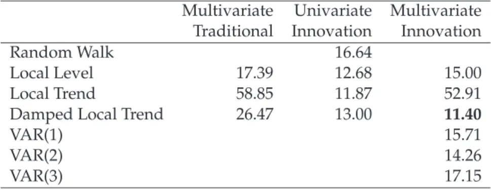
The results shown in Table2indicate that the random walk works well. Its performance is similar to the local level models. It is not as good, however, as the multivariate innovation damped trend model.
Multivariate Univariate Multivariate
Traditional Innovation Innovation
Random Walk 16.64
Local Level 17.39 12.68 15.00
Local Trend 58.85 11.87 52.91
Damped Local Trend 26.47 13.00 11.40
VAR(1) 15.71
VAR(2) 14.26
VAR(3) 17.15
Table 2: Comparison of approaches: mean absolute scaled error. The bolded value denotes the minimum value.
As stated previously, this new innovation approach is an alternative to the traditional form postulated by Harvey (1989). Such models differ from their innovation counterparts in that they rely on multiple sources of uncorrelateddisturbances. The results in Table2
indicate that the innovation approach out-performed the multiple disturbance state space approaches. In theory, for a restricted range of parameter values, the approaches are known to be equivalent. However, the innovation models can take parameter values that have no counterpart in the uncorrelated multi-disturbance models. Some of the estimated parameter values turned out to belong in this region. This illustrates the point that the innovation framework can be more flexible than its multi-disturbance counterpart.
The innovation and multi-disturbance form of the local trend model both performed no-ticeably poorly when compared to their univariate innovation counterpart. In the fol-lowing section, which evaluates the multivariate innovation form, no such observation is made. Moreover the results suggest that the innovation local trend model is relatively accurate when compared to the univariate form, especially in small samples.
The VAR is another alternative. The VARs considered were restricted to have one, two or three lags. The maximum number of lags was set to three because this corresponds to the number of unknowns in the vector damped local trend model. As prior testing of the series revealed that the log of the series was non-stationary, the VAR models were fitted to the first difference of the logs. The results indicate that the VISTS approach forecasts better than the VAR approach for this particular set of data.
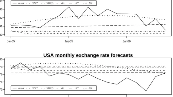
UK monthly exchange rate forecasts
UKP/AUD 0.40 0.41 0.42 0.43 0.44
Jan05 July05 Jan06
Actual VDLT VAR(2) MLL ULT RW
USA monthly exchange rate forecasts
USD/AUD 0.72 0.74 0.76 0.78 0.80
Jan05 July05 Jan06
Actual VDLT VAR(2) MLL ULT RW
Figure 2:Predicted monthly exchange rates.
Figure2displays the monthly Australian exchange rates for the UK pound and the Amer-ican dollar for the period of the holdout sample . The observations are indicated by the solid line in both panels. The forecasts for the vector damped local trend, VAR and con-ventional local level models are also displayed. The trajectory of the vector damped local
trend forecast is particularly impressive, closely following the seventeen monthly obser-vations of the UKP/AUD exchange rate following December 2004. The forecast of the USD/AUD exchange rates is marginally inferior at some horizons, however, overall the vector damped local trend model produces the most accurate forecasts (Table2).
Model AIC
Vector local level -13.608
Vector local trend -13.628
Vector damped local trend -13.763
Table 3:Akaike Information Criterion of the fitted VISTS models.
On fitting a family of models, it is common practice to use the AIC to make the choice of which model to use for forecasting. The VAR(3) had the lowest AIC value amongst the VARs; however, it produced forecasts inferior to the VAR(1) and VAR(2). The damped trend had the lowest AIC amongst the VISTS models and produced the most accurate forecasts (Tables2 & 3). Therefore we can conclude that the AIC correctly anticipated the forecasting capacities of the VISTS models. This is consistent with the findings of Billah et al. (2005) on the relationship between information criteria and the forecasting performances of various forms of exponential smoothing.
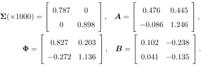
The parameter estimates of the vector damped local trend model are:
Σ(×1000) = 0.787 0 0 0.898 , A= 0.476 0.445 −0.086 1.246 , Φ= 0.827 0.203 −0.272 1.136 , B = 0.102 −0.238 0.041 −0.135 .
In general, the parameters withinΦ,A andB denote various elasticities. It is difficult to draw any specific conclusions using the parameter estimates because the states and series interact. Importantly, the modulus of the largest eigenvalue is less than one (al-beit marginally), and therefore the dampening characteristic of the trend is captured. To determine the various inter-relationships of a model, the impulse response function, a common multivariate time series analysis tool, is used (see L ¨utkepohl, 2005). The
im-δ. Typically the unexpected change (or shock) is set to be one standard deviation of the residuals. Its size is set to 1 in the following analysis. Formally, the impulse response function (Koop, Pesaran and Potter, 1996) is defined as
=y(n,δ,It−1) = E(yt+n|et=δ,et+1 =0, . . . ,et+n=0)− E(yt+n|et=0,et+1=0, . . . ,et+n=0)
whereIt−1contains all the information upon which the distribution ofytis conditioned. It is calculated assuming that no shock is experienced between the periodstandt+n, except forδat timet. As the errors are assumed to be contemporaneously independent,
δdenotes anN-vector with one element equal to the size of the shock and the remaining cells set to zero.
Unlike the standard VAR framework, two forms of impulse response function analysis can be performed. The first is the standard form where the response in the observations is gauged. The second is the ability to disaggregate the observed response into its latent states. This is particularly interesting in the vector damped local trend case, as it provides the means to distinguish between temporary (local growth) and permanent (local level) fluctuations. An important feature of this specification is that the temporary component feeds directly into the level.
The impulse response functions are first presented in the standard form, followed by the state decomposition of the responses. The size of the shock represents a 1% apprecia-tion in the exchange rate. The shocks are analysed independently, beginning with the UKP/AUD exchange rate.
A key feature of the impulse response functions is the longevity of the unanticipated appreciations. Only the 36 months immediately following the shocks are mapped in Figure 3. When the horizon is extended, the response does not settle down for some considerable time, indicating that both series are sensitive to unanticipated changes and have characteristics in common with long memory processes.
There are two other interesting features of the mapped responses in regard to their shape. The first is the cyclical nature of the reaction. The second is that the trajectories of the reactions of each exchange rate are very similar. The cyclical character of the response
0 5 10 15 20 25 30 35 −0.2 0.0 0.2 0.4 0.6 0.8 1.0
A: UKP/AUD Response UKP/AUD Shock
Month Impact, % 0 5 10 15 20 25 30 35 −1.4 −1.2 −1.0 −0.8 −0.6 −0.4 −0.2 0.0
B: USD/AUD Response UKP/AUD Shock
Month Impact, % 0 5 10 15 20 25 30 35 −0.5 0.0 0.5 1.0 1.5
C: UKP/AUD Response USD/AUD Shock
Month Impact, % 0 5 10 15 20 25 30 35 1.0 1.5 2.0 2.5 3.0 3.5 4.0
D: USD/AUD Response USD/AUD Shock
Month
Impact, %
Figure 3:Observed reaction to a 1% unanticipated appreciation.
implies the adjustments are a series of over- and under-shooting episodes before the new equilibrium reached. The similar shapes of the response mechanisms suggest the series considered are closely associated.
The second set of impulse response functions (Figure 4) represents the reaction in the permanent and temporary components of the variables under consideration. In general, the panels illustrate that the UKP/AUD and USD/AUD respond similarly to a given unanticipated change.
The permanent and temporary natures of the level and trend components could be illus-trated by extending the horizon of the functions in Figure4. This would show that the cyclical responses in panels C and D eventually decay (in magnitude) to zero. In con-trast, the cyclical fluctuations plotted in panels A and B never return to zero, but decay (in magnitude) to new equilibrium values.
0 5 10 15 20 25 30 35 −1.5 −1.0 −0.5 0.0 0.5
1.0 A: Smoothed Averages (UKP/AUD shock)
Month Impact, % 0 5 10 15 20 25 30 35 −0.10 −0.05 0.00 0.05 0.10
C: Smoothed Growth Rates (UKP/AUD shock)
Month Impact, % 0 5 10 15 20 25 30 35 0 1 2 3 4
B: Smoothed Averages (USD/AUD shock)
Month Impact, % 0 5 10 15 20 25 30 35 −0.2 −0.1 0.0 0.1 0.2
D: Smoothed Growth Rates (USD/AUD shock)
Month
Impact, %
Figure 4:Latent component reaction to a 1% shock. (—) UKP/AUD, (- -) USA/AUD.
Shock UKP/AUD USD/AUD
UKP/AUD 0.30% 0.60%
USD/AUD -0.70% 2.50%
Table 4: Permanent adjustments with respect to a 1% appreciation.
a 1% shock in the UKP/AUD exchange rate results in a long term adjustment of 0.30% and 0.60% in the UKP/AUD and USD/AUD exchange rates. These values can be con-sidered as long-run elasticities. In general, the values show that for three out of the four instances, the adjustment is less than 1%. In both cases it appears that the USD/AUD exchange rate is more sensitive to shocks, experiencing greater changes in magnitude.
Figure5displays the latent components for the months over the period January 2000 to December 2004. The level was transformed by taking the anti-log, and therefore rep-resents the smoothed value. The smoothed growth rates of the series are displayed in panels C and D.
A: UKP/AUD Smoothed Average Time Smoothed Average 0.34 0.36 0.38 0.40 0.42 2000 2001 2002 2003 2004 2005
B: USD/AUD Smoothed Average
Time Smoothed Average 0.50 0.55 0.60 0.65 0.70 0.75 2000 2001 2002 2003 2004 2005
C: UKP/AUD Smoothed Growth Rate
Time % −2 −1 0 1 2 2000 2001 2002 2003 2004 2005
D: USD/AUD Smoothed Growth Rate
Time % −2 −1 0 1 2 2000 2001 2002 2003 2004 2005
Figure 5:Estimated components of the series, spanning January 2000 to December 2004.
was followed by a sharp correction early in 2004, which was preempted by smoothed negative growth rates of 2% and 1% for the UKP/AUD and USD/AUD exchange rates respectively. Panels A and B clearly show that the correction did not shift the average of either exchange rate, as they returned to their previous levels shortly after the correction, with smoothed growth rates reaching nearly 2% for both series.
Figure5displays one valuable feature of the VISTS framework, the calculation of filtered components within the model building process. Filtered or smoothed components high-light the salient features of the variables of interest, and are therefore useful in examining the effects of past events on the data.
In summary, this section illustrates that the VISTS framework generates accurate fore-casts and reveals important and previously undetectable information regarding the vari-ables being fitted. In particular, it is shown that this new alternative framework combines the best features of the VAR and traditional structural time series models, namely simple implementation and useful interpretation.
5 Forecasting experiment
To dispense with the possibility that the better performance of the VISTS model in the previous study was simply due to chance, an extensive forecasting study was undertaken to examine the robustness of the approach on a large number of series. In particular, four aspects are considered:
1 The advantages of a multivariate verses a univariate framework.
2 The accuracy of the VISTS specification verses the traditional structural time series specifications.
3 The predictive ability of the VISTS framework compared to the most common al-ternative VAR.
4 A general comparison combining aspects 1 and 3 using an automatic model selec-tion procedure.
The forecasting accuracy of all models is evaluated once using 1000 different data sets. The variables and their starting dates are randomly chosen from the Watson (2003) macroeconomic database. The Watson (2003) database comprises eight groups which can be loosely considered to represent different economic sectors. The number of variables in each group ranges from 13 to 27. All variables are real and non-seasonal, with obser-vations from January 1959 to December 1998. Every data set comprises two randomly chosen, variables from different economic sectors. The starting date is randomly chosen where the only restriction is that there must be enough observations to fit and evaluate out-of-sample forecasts up to twelve horizons.
Two sizes of estimation sample are considered, 30 and 100. These sample sizes were chosen because they resemble small and large sample sizes that occur in practice. All variables are standardised by dividing by the standard deviation of their first difference.
The forecasts of the three VISTS models are compared to three alternatives: VAR models, traditional structural time series models and univariate innovation structural time series models. All three approaches have been established for some time and are commonly used.
The multivariate form of the ARIMA methodology is confined to a vector autoregression (VAR) (L ¨utkepohl, 2005) with at most three lags fitted to the first difference of the data. An upper limit of three lags was set as this corresponds to the largest VISTS model the damped local trend model. The optimal lag length is determined using the multivariate form of the AIC.
The number of multiple source of error structural time series models available to the forecaster is quite large; however, here it is strictly limited to the equivalent of the vector local level, vector local trend and vector damped local trend models. These models are denoted the TLL, TLT and TLDT respectively. Table 5 lists the full set of alternatives considered.
Model Description
VLL Vector local level model VLT Vector local trend model VLDT Vector local damped model VAR Vector autoregression
TLL Traditional multivariate local level multiple source of error model TLT Traditional multivariate local trend multiple source of error model
TLDT Traditional multivariate local damped trend multiple source of error model UISTS Univariate innovation structural time series models
Table 5:Index of time series models included in forecasting experiment.
As before, we average the MASE over the two series for each data set, and over each horizon. The maximum horizon length considered is twelve.
5.1 Results
Multivariate verses univariate innovation structural time series models
In this first section a comparison is made between the univariate and multivariate in-novation structural time series models. The objective of this comparison is to determine whether there is any advantage in extending the univariate form into a multivariate spec-ification.
Horizon VLL VLT VLDT ULL ULT ULDT 1 15.6 21.3 19.7 13.3 15.9 14.2 2 13.7 22.3 19.4 13.0 16.5 15.7 3 12.6 23.7 20.4 12.1 16.5 14.7 4 11.1 23.5 19.7 10.8 19.0 15.9 5 11.1 22.3 20.2 9.4 20.2 16.8 6 9.9 21.8 20.5 9.8 21.9 16.1 7 11.0 22.1 18.9 9.2 21.5 17.3 8 10.4 22.4 17.9 9.2 21.4 18.7 9 10.3 22.4 18.0 9.3 21.4 18.6 10 9.4 22.5 18.1 9.5 21.6 18.9 11 9.4 22.4 18.2 9.5 21.5 19.0 12 9.0 22.1 19.1 9.6 21.5 18.8 Average 11.1 22.4 19.2 10.4 19.9 17.1
Table 6:Percentage of first ranks, sample size 30. The largest proportion in each row is bolded.
Horizon VLL VLT VLDT ULL ULT ULDT
1 13.5 24.7 19.9 13.6 16.2 12.1 2 11.9 22.7 23.3 12.9 18.3 12.3 3 10.1 23.9 24.1 9.6 19.7 12.6 4 9.1 23.8 23.4 9.3 21.1 13.6 5 8.4 22.5 24.2 8.7 21.2 15.0 6 9.0 22.3 22.3 8.9 22.7 14.9 7 8.2 21.7 21.4 9.5 23.1 16.1 8 8.0 21.5 21.2 9.3 23.4 16.6 9 8.0 21.4 21.5 8.7 23.5 16.9 10 8.5 20.8 21.4 8.6 23.1 17.7 11 8.1 20.4 21.3 9.4 23.1 17.7 12 7.7 20.7 21.5 9.4 22.6 18.1 Average 9.2 22.2 22.1 9.8 21.5 15.3
the vector local trend (VLT) model produced the most accurate forecast at the twelve step ahead horizons in the small sample application 22.1% of the time.
In general, the vector local trend model appears to be the most accurate, registering the highest average in both tables. The second most accurate model depends on which sam-ple size is being considered. In the large samsam-ple case the vector damped local trend model is the second most accurate model (as indicated by the average), whereas it is the third most accurate model in the small sample size context, behind the univariate and vector local trend models. The VLL model appears to produce the least accurate predictions in general.
Overall, all models perform well, at times outperforming the alternatives considered. It is however evident that VISTS has a slight advantage over its univariate counterpart.
The vector models that contain a local trend outperform their univariate counterpart across most horizons. The results presented in the above tables illustrate that the vec-tor models have produced more accurate forecasts on a regular basis.
local level local trend damped local trend
−1 0 1 2
Small sample size forecast comparison, short horizon
Multivariate−Univariate
local level local trend damped local trend
−1.0 −0.5 0.0 0.5 1.0
Large sample size forecast comparison, short horizon
Multivariate−Univariate
local level local trend damped local trend
−2 0 2 4 6
Small sample size forecast comparison, long horizon
Multivariate−Univariate
local level local trend damped local trend
−2 −1 0 1 2 3
Large sample size forecast comparison, long horizon
Multivariate−Univariate
Figure6displays the relative accuracy of the multivariate versus the univariate specifi-cation by model. The middle 98% band of discrepancies is presented, as there are a few extreme values that make the chart difficult to interpret. A positive discrepancy indicates that the multivariate version of the model is less accurate. The differences are calculated for the short and long horizons corresponding to three and twelve step ahead forecasts.
The box and whisker plots indicate that the degree of forecast accuracy of the univariate and multivariate procedures are similar. The vector local level model is particularly in-teresting as the median difference is always slightly negative, indicating that it is more accurate than the univariate alternative. In most cases, the median is approximately zero, indicating that for half of the comparisons the multivariate model outperformed its uni-variate equivalent.
In summary, the results in Tables 6and7indicate that the VISTS models generated the most accurate forecasts for over 50% of the comparisons. Furthermore, the discrepancies displayed in Figure 6 indicate that the forecasts from the VISTS models are relatively robust. Therefore, it is concluded that there is an advantage in extending the framework from a univariate to a multivariate specification.
VISTS verses the traditional structural approach
In this section the VISTS framework is compared to the traditional form of the structural time series model (also referred to as SUTSE). The traditional form is characterised by multiple sources of error and is arguably more tedious to implement.
Tables 8and9display the percentages of first places for each model over horizons one to twelve. The maximum percentage in each row is bolded. As is consistent with the previous findings, the vector local trend model appears to have produced the most ac-curate forecasts more often than any of the alternatives in the small sample size context (but not the highest average in the large sample case). The vector damped local trend model was second to the vector local trend model in the large sample case. The VISTS models that are characterised by a local trend outperformed their traditional structural form equivalents over all horizons except the first in the context of a large sample size.
Horizon VLL VLT VLDT TLL TLT TLDT 1 12.4 17.4 16.8 14.1 25.3 14.0 2 12.1 19.6 18.3 13.1 21.9 15.7 3 11.1 20.8 19.1 12.7 20.2 16.1 4 10.9 21.5 18.8 11.3 20.4 17.3 5 10.3 21.1 19.9 10.4 21.1 17.2 6 10.2 20.9 20.6 9.9 21.2 17.2 7 10.4 21.6 20.3 9.3 20.6 17.8 8 9.9 21.6 20.4 9.3 20.4 18.4 9 9.6 21.9 19.9 9.6 20.8 18.2 10 9.2 21.6 19.9 9.1 21.4 18.8 11 8.9 21.6 20.8 9.5 21.1 18.1 12 8.8 21.8 21.0 8.9 21.3 18.2 Average 10.3 21.0 19.7 10.6 21.3 17.3
Table 8: Percentage of first places, small sample size. The largest proportions for each row are in bold. Horizon VLL VLT VLDT TLL TLT TLDT 1 9.5 22.0 18.5 14.1 24.0 11.9 2 9.7 23.2 20.4 13.1 21.0 13.4 3 7.3 26.9 21.3 11.5 20.7 12.3 4 7.3 26.8 23.2 10.6 20.0 12.2 5 7.7 25.7 21.7 10.4 21.1 13.4 6 7.7 26.5 21.7 10.3 20.6 13.3 7 7.6 25.8 22.8 10.0 20.7 13.1 8 7.5 25.7 22.4 9.9 20.4 14.1 9 7.1 25.7 23.2 9.8 20.1 14.1 10 7.0 25.5 22.9 9.9 20.8 13.9 11 7.1 25.5 22.9 10.2 20.1 14.2 12 7.1 26.7 23.2 9.6 19.3 14.1 Average 7.7 25.5 22.0 10.8 20.7 13.3
Table 9: Percentage of first places, large sample size. The largest proportions for each row are in bold.
Again it is apparent that all models considered experience some degree of success. More-over, the innovation models appear to perform slightly better that their traditional coun-terparts.
Figure 7 illustrates the middle 98% band of discrepancies of the VISTS and the tradi-tional state space models on a model specific basis. The long and short horizons refer to
local level local trend damped local trend −1
0 1 2
Small sample size forecast comparison, short horizon
VISTS−Conventional
local level local trend damped local trend
−2 −1 0 1
Large sample size forecast comparison, short horizon
VISTS−Conventional
local level local trend damped local trend
−6 −4 −2 0 2 4 6
Small sample size forecast comparison, long horizon
VISTS−Conventional
local level local trend damped local trend
−6 −4 −2 0 2 4
Large sample size forecast comparison, long horizon
VISTS−Conventional
Figure 7:Discrepancies in MASE, VISTS-conventional state space model.
the forecast performance for twelve and three steps ahead respectively. The most strik-ing feature of these charts is that the median difference is at or below zero in almost all instances, indicating that the VISTS model generates a more accurate forecast than the conventional structural time series model equivalent at least 50% of the time. In gen-eral, the charts indicate that the degree of forecasting accuracy is similar between these opposing methodologies, indicating that the VISTS forecasts are relatively robust.
In summary, the VISTS approach is arguably a simpler and more flexible form than the traditional structural time series model, and has been shown to produce accurate and robust forecasts on a regular basis. Therefore the evidence suggests that the VISTS model is not just a worthy alternative, but a good substitute for time series analysts wanting to employ a structural time series approach.
Comparison with VAR
The objective of this comparison is to gauge the forecasting accuracy of the VISTS frame-work against what is arguably the most popular multivariate time series modeling tool, the VAR approach. Both methods include an automatic model selection procedure using the AIC.
Small sample Large sample
Horizon VISTS VAR VISTS VAR
1 48.3 51.7 51.1 48.9 2 48.7 51.3 52.1 47.9 3 49.4 50.6 53.8 46.2 4 48.5 51.5 53.9 46.1 5 48.0 52.0 52.6 47.4 6 47.4 52.6 51.7 48.3 7 47.4 52.6 52.0 48.0 8 47.6 52.4 51.7 48.3 9 47.8 52.2 53.0 47.0 10 47.8 52.2 53.9 46.1 11 48.3 51.7 54.0 46.0 12 47.5 52.5 53.6 46.4 Average 48.1 51.9 52.8 47.2
Table 10:Percentage of first places.
Table 10 displays the relative predictive performance of VAR and VISTS models using an automatic model selection procedure. The VAR framework was fitted to the first dif-ferences of the data. The maximum order permitted was three lags for the VAR, as this reflects the number of unknown parameters in the vector damped local trend model. The overall results are quite similar, with the VISTS slightly outperforming the VAR in the large sample and vice-versa in the small sample.
The box and whisker plots in Figure8display the middle 98% band of forecasting dis-crepancies between the VAR and VISTS models. The long and short horizon plots illus-trate the relative predictive accuracy at twelve and three steps ahead respectively. As is consistent with previous findings, the median is at zero and the distribution is sym-metrical about this point. This indicates overall, that neither of the approaches perform particularly badly.
Small sample Large sample −1.5 −1.0 −0.5 0.0 0.5 1.0 1.5
Forecast comparison, short horizon
VISTS−VAR
Small sample Large sample −4 −2 0 2 4 6
Forecast comparison, long horizon
VISTS−VAR
Figure 8:Discrepancies in MASE, VISTS-VAR.
In summary, these results show the VISTS framework to be a worthy alternative to the standard time series techniques. From Table 10 and Figure 8it is clear that the VISTS model produces accurate forecasts on a regular basis. Furthermore, the distribution of the box and whisker plots displayed in Figure8indicates that the forecasts are robust.
Automatic model selection
This final comparison considers all the alternatives except the traditional structural time series models. The objective is to determine which (if any) of the approaches that include an automatic model selection feature produced a relatively higher degree of forecasting accuracy.
Table11displays the percentage of times that each alternative is most accurate. It is clear that all three approaches perform relatively well.
Small Sample Large Sample
Horizon VISTS UISTS VAR VISTS UISTS VAR
1 29.9 35.7 34.4 31.9 33.5 34.6 2 31.0 37.4 31.7 33.5 34.5 32.2 3 31.4 38.3 30.3 34.3 35.5 30.2 4 30.7 38.9 30.4 33.5 36.3 30.2 5 30.0 39.3 30.7 31.2 38.6 30.2 6 29.8 39.3 30.9 30.6 38.3 31.1 7 30.9 37.9 31.2 31.5 37.5 31.0 8 31.0 37.6 31.4 32.4 37.2 30.4 9 31.5 38.0 30.5 32.3 38.4 29.3 10 30.7 38.4 30.9 32.8 39.3 27.9 11 30.1 39.6 30.3 33.0 38.8 28.2 12 30.1 39.1 30.8 32.9 38.8 28.3 Average 30.6 38.3 31.1 32.5 37.2 30.3
Table 11:Percentage of first places.
In particular, the results show that the univariate innovation structural time series ap-proach outperformed the multivariate alternatives across all horizons. The relative per-formances of the VISTS and VAR approaches are consistent with the findings in the pre-vious section: VISTS performed relatively better when fitted to the larger sample.
Figure 9 displays the forecast discrepancy between the VISTS, VAR and UISTS frame-works. In all three cases, automatic model selection took place using the AIC. The mid-dle 98% band of forecasting discrepancies is pictured. In all instances, the range of the box and whisker plots indicates that the relative degree of forecasting accuracy is similar, thereby indicating that the VISTS framework produced robust forecasts.
In general, the results here and in the previous sections show the VISTS framework to be a worthy alternative when compared to the forecasting tools considered. For each com-parison, the VISTS framework produced the most accurate forecasts on a consistent basis (approximately 50% of the time). Furthermore, the box and whisker plots illustrate that the forecasts are generally robust. Therefore, on the basis of this evidence, it is concluded that the VISTS framework is a valuable tool and can be considered a viable multivariate time series forecasting approach.
UISTS−Short Hor. VAR−Short Hor. UISTS−Long Hor. VAR−Long Hor. −2 0 2 4 6
Forecast comparison, small sample
VISTS−Alternative
UISTS−Short Hor. VAR−Short Hor. UISTS−Long Hor. VAR−Long Hor. −2
0 2 4 6
Forecast comparison, large sample
VISTS−Alternative
Figure 9:Discrepancies in MASE, VISTS-Automatic model selection alternatives.
6 Conclusion
The vector version of the innovation state space model was introduced and evaluated as a mechanism for forecasting related macroeconomic time series. It was contrasted with the vector autoregressive and conventional state space approaches which are typically used in multiple time series studies. By conditioning on seed states rather than an initial run of series values, it was shown that maximum likelihood estimates could be obtained with a simple recursion reminiscent of exponential smoothing. It was also shown that the effect of shocks could be tracked, not only on the series itself, but on the components from which the series is constituted. Some preliminary empirical studies indicated that VISTS is a robust approach to forecasting and performs better than the conventional approaches in a significant proportion of cases.
movements in time series reminiscent of those that have been the focus of the co-integration literature. Other work will be directed to generalising the univariate frame-work in Hyndman et al. (2002) so that seasonal effects, non-linear relationships and het-eroscedastic error processes are accommodated
References
Anderson, B. and J. B. Moore (1979)Optimal Filtering, Prentice-Hall.
Ansley, C. F. and R. Kohn (1985) Estimation, filtering and smoothing in state space models with incompletely specified conditions,Annals of Statistics,13, 1286–1316.
Billah, B., M. King, R. Snyder and A. Koehler (2005) Exponential smoothing model selec-tion for forecasting, Working paper, Monash University, Australia.
Brown, R. G. (1959)Statistical forecasting for inventory control, McGraw-Hill, New York.
Clarida, R., L. Sarno, M. Taylor and G. Valente (2003) The out-of-sample success of term structure models as exchange rate predictors: one step along,Journal of International Economics,60, 61–83.
de Jong, P. (1991) The diffuse Kalman Filter,Annals of Statistics,19, 1073–1083.
Gardner, E. S. and E. McKenzie (1985) Forecasting trends in time series,Management Sci-ence,31, 1237–1246.
Granger, C. W. and P. Newbold (1986) Forecasting economic time series, Academic Press, New York, 2nd ed.
Hannan, E. J. and M. Deistler (1988)The statistical theory of linear systems, John Wiley & Sons.
Harvey, A. and S. Koopman (1997) Multivariate structural time series model, inSystem Dynamics in Economic and Financial Models, pp. 269–296.
Harvey, A. C. (1989) Forecasting, structural time series models and the Kalman filter, Cam-bridge University Press, CamCam-bridge.
Hyndman, R. and A. B. Koehler (2005) Another look at measures of forecast accuracy, Working paper, Department of Econometrics and Business Statistics, Monash Univer-sity, Australia.
Hyndman, R. J., A. B. Koehler, R. D. Snyder and S. Grose (2002) A state space framework for automatic forecasting using exponential smoothing methods,International Journal of Forecasting,18(3), 439–454.
Koop, G., M. H. Pesaran and S. M. Potter (1996) Impulse response analysis in nonlinear multivariate models,Journal of Econometrics,74, 119–147.
L ¨utkepohl, H. (2005)New Introduction to Multiple Time Series Analysis, Springer-Verlag.
Meese, R. and K. Rognoff (1983) Empirical exchange rate model of the seventies,Journal of International Economics,14, 3–24.
Ord, J. K., A. B. Koehler and R. D. Snyder (1997) Estimation and prediction for a class of dynamic nonlinear statistical models,Journal of the American Statistical Association, 92, 1621–1629.
Snyder, R. D. (1985) Recursive estimation of dynamic linear statistical models,Journal of the Royal Statistical Society (B),47(2), 272–276.
Watson, M. (2003) Macroeconomic forecasting using many predictors, inAdvances in Eco-nomics and Econometrics, Theory and Applications, Eighth World Congress of the Econometric Society, vol. 3, pp. 87–115.