Aerothermodynamic Testing and Boundary Layer Trip Sizing of the
HIFiRE Flight 1 Vehicle
Karen T. Berger* and Frank A. Greene† NASA Langley Research Center, Hampton, VA, 23681
and
Roger Kimmel‡
Air Vehicles Directorate, Air Force Research Laboratory, Dayton, OH
An experimental wind tunnel test was conducted in the NASA Langley Research Center’s 20-Inch Mach 6 Air Tunnel in support of the Hypersonic International Flight Research Experimentation Program. The information in this report is focused on the Flight 1 configuration, the first in a series of flight experiments. This report documents experimental measurements made over a range of Reynolds numbers and angles of attack on several scaled ceramic heat transfer models of the Flight 1 payload. Global heat transfer was measured using phosphor thermography and the resulting images and heat transfer distributions were used to infer the state of the boundary layer on the vehicle windside and leeside surfaces. Boundary layer trips were used to force the boundary layer turbulent, and a brief study was conducted to determine the effectiveness of the trips with various heights. The experimental data highlighted in this test report were used to size and place the boundary layer trip for the flight test vehicle.
Nomenclature
AoA angle of attackD diameter
h Heat transfer coefficient (lbm/ft2-sec)
( w
H
H
q
−
&
) H enthalpy (BTU/lbm)href reference heat-transfer coefficient using
Fay-Riddell
k boundary-layer trip height (in) Lref reference length (in)
P pressure, psia
q dynamic pressure (psi)
q
&
heat transfer rate (BTU/ft2-sec)r radius (in)
Re unit Reynolds number (1/ft)
Rextrip Length Reynolds number based on trip
location
t time (sec)
T temperature (°F)
x axial distance from origin (in) y lateral distance from origin (in)
α angle of attack (deg)
β sideslip angle (deg)
δ boundary-layer height (in)
δ∗ displacement thickness (in)
µ viscosity (slug/ft-sec)
Subscripts
1 free-stream conditions aw adiabatic wall
n model nose
ref reference value t,1 reservoir condition
t,2 stagnation conditions behind normal shock w wall
∞ free-stream conditions
I.
Introduction
The Hypersonic International Flight Research Experimentation (HIFiRE) program is a joint hypersonic flight test program between the Air Force Research Laboratories (AFRL) and Australian Defence Science and Technology ________________
* Aerospace Engineer, Aerothermodynamics Branch, MS 408A, Member.
†
Aerospace Engineer, Aerothermodynamics Branch, MS 408A, Member‡
Research Aerospace Engineer,Air Vehicles Directorate, Associate FellowOrganization (DSTO) with input from universities, private industry and NASA. The goal of the HIFiRE program is to develop and demonstrate fundamental hypersonic technologies for application to advanced scramjet powered vehicles. This will be accomplished through a series of launches incorporating flight experiments to demonstrate basic and applied research concepts for hypersonic scramjet flight. The program will span 6 years and include flights of Mach 5 and above. The flight tests will be conducted at the Woomera Prohibited Test Range, in Southern Australia. The primary goal of the HIFiRE Flight 1 experiment is to obtain transitional and turbulent boundary layer heating flight data. The payload is a 7-deg cone-cylinder-flare configuration and approximately 6.3 feet in length at full scale. The test flight is scheduled for early 2008.
The primary objective of the test entry into the Langley Research Center (LaRC) 20-Inch Mach 6 Air Tunnel was to determine the effective boundary layer trip size and the effect of the turbulent flow due to the discrete roughness elements, similar to that which will be used on the flight vehicle. A series of cast ceramic models were fabricated. Global phosphor thermography was used to obtain the surface heating rates at Reynolds numbers between 2.1x10⁶/ft and 5.6x10⁶/ft and angles of attack from -5 to +5 deg. Boundary layer trips were required for this
test, as the flight vehicle will incorporate a single boundary layer trip on one side to ensure that a portion of the flight will generate turbulent heating data. The data were also used to determine the location of flight instrumentation (not discussed in this paper). Comparisons of experimental data with computational fluid dynamics (CFD) predictions will also be presented. The effects of the flare angle and duct on the heating levels were also investigated. Testing focused on the wind-side and leeside surfaces of the models.
II.
Experimental Methods
A. Model/Support Hardware
The HIFiRE Flight 1 Payload Outer Mold Line (OML) is a 7-deg cone with a cylinder-flare afterbody. The vehicle has a nose radius of 0.098 in. and a full scale length of 75.45 in. A reference flight vehicle OML is shown in Fig. 1 (Table 1 contains nominal model parameters).
Figure 1: HIFiRE Flight 1 Payload OML and Dimensions (in)
Five different model configurations were fabricated for this test; three for the full-vehicle and two of the forecone only. All models were 15 in. long. The three full-vehicle models had a scale of 19.84% except in the nose radius where fabrication difficulties limited the ability to fabricate the nose with the correct scaled radius. The nose radius of all three full-vehicle models was 0.047 in. and when compared to the full scale nose radius of 0.0984 in. resulted in a model nose radius scale of 47.8%. Two of the full-vehicle models had flare angles of 33 deg (one with and one without the duct) and the third full-vehicle model had a flare angle of 37 deg (with the duct). The duct will be used for an optical mass-capture experiment in flight. The two forecone models were 34.7% scale models of the forecone section of the vehicle with the exception of their nose radii. One radius was sized to match the physical size of the full vehicle models, 0.047 in. and the other was scaled up with the rest of the forecone from the full vehicle model, resulting in a nose radius of 0.083 in. The two different nose radii allow for the investigation of the effect of nose radius variation.
The cast ceramic models used in the Mach 6 test series were manufactured from molds created from rapid prototyped resin patterns. Standard methods, materials, and equipment developed at NASA LaRC were used in fabricating the ceramic aeroheating test models.1 Due to the relative symmetry of the HIFiRE models, casting molds
were created directly from the resin patterns bypassing the wax pattern requirement. This step is note worthy, as in general it has been determined that shrinkage in the wax patterns introduce the largest uncertainty in the final
Duct
ceramic OML. All models were supported by 1-in. diameter cylindrical stainless steel straight stings mounted through the axis of symmetry. Fiducial marks were applied to the model surface using a coordinate measuring machine. The reference marks on the model surface were used to align the model in the tunnel for testing and to aid in data reduction using the phosphor thermography system. Nominal model installations can be seen in Fig. 2.
Table 1: Model Reference Dimensions (for all models, length was 15 in.) Model Name Configuration
Cylinder Diameter (in) Base Diameter (in) Nose Radius (in) Flare Angle (deg) Base/Sting Diameter Duct 33 deg w/ channel CCF33D Full vehicle 2.14 2.77 0.047 33 2.77 Yes 33 deg w/o channel CCF33 Full vehicle 2.14 2.77 0.047 33 2.77 No
37 deg w/ channel CCF37D Full vehicle 2.14 2.77 0.047 37 2.77 Yes Forecone 0.047 NR 047 Cone Forecone NA 3.75 0.047 NA 3.75 NA Forecone 0.083 NR 083 Cone Forecone NA 3.75 0.083 NA 3.75 NA
(a) (b)
Figure 2: Model Set-Up for testing in the Mach 6 Tunnel: (a) Full Vehicle and (b) Forecone Models
B. Facility
20-Inch Mach 6 Tunnel: The Langley 20-Inch Mach 6 Tunnel2 is a blow down wind tunnel that uses dry air as the test gas (that has well characterized perfect gas flows in terms of composition and uniformity). Air from two high pressure bottle fields is transferred to a 600-psia reservoir and is heated to a maximum temperature of 1000°R by an electrical resistance heater. A double filtering system is employed having an upstream filter capable of capturing particles larger than 20 microns and a second filter rated at 5 microns. The filters are installed between the heater and settling chamber. The settling chamber contains a perforated conical baffle at the entrance and internal screens; the maximum operating pressure is 525 psia. A fixed geometry, two-dimensional contoured nozzle is used; the top and bottom walls of the nozzle are contoured and the sides are parallel. The nozzle throat is 0.34 in. by 20 in., the test section is 20.5 in. by 20 in., and the nozzle length from the throat to the test section window center is 7.45 ft. This tunnel is equipped with an adjustable second minimum and exhausts either into combined 41-ft diameter and 60-ft diameter vacuum spheres, a 100-ft diameter vacuum sphere, or to the atmosphere through an annular steam ejector. The maximum run time is 20 minutes with the ejector, though heating tests generally have total run times of 30 sec, with actual model residence time on tunnel centerline of approximately 5-10 sec. Models are mounted on the injection system located in housing below the closed test section. This system includes a computer operated sting support system capable of moving the model through an angle of attack range of -5 to +55 deg and angles of sideslip of ±8 deg. Flow conditions were acquired using a 16-bit analog-to-digital facility acquisition system. The values of Pt,1 and Tt,1 are
believed to be accurate to within ±2%. The uncertainties in the angle of attack of the model are believed to be ±0.2º.
C. Experimental Methods
Global Phosphor Thermography: The two-color relative-intensity phosphor thermography measurement technique was used to obtain global experimental aeroheating data in the tunnel3-5. This technique uses a mixture of phosphors
that fluoresce in the bands of the visible spectrum when illuminated with ultraviolet light. The red and green bands are used and the intensity of the fluorescence is dependent upon the amount of incident ultraviolet light and the local surface temperature of the phosphor. This phosphor mixture, which is suspended in a silica ceramic binder and applied with an air brush, is used to coat a slip cast silica ceramic model. The final coating thickness is approximately 0.001 in. Using a 3-CCD (Charge Coupled Device) camera, fluorescence intensity images of an illuminated phosphor model exposed to the heated hypersonic flow of the tunnel are acquired and converted to temperature mappings via a temperature-intensity calibration. The temperature-intensity calibration uses the ratio of the red and green components of the image to construct a lookup table which converts the intensities to temperature
value. Currently, this calibration is valid over a temperature range from 532 °R to 800 °R. The temperature data from the time-sequenced images taken during the wind tunnel run are then reduced to enthalpy based heat transfer coefficient at every pixel on the image (and hence globally on the model) using a heat-transfer calculation assuming one-dimensional semi-infinite slab heat conduction4.
D. Data Presentation, Quality and Uncertainty
Global heating images and corresponding centerline data cuts will be presented in the non-dimensional h/href
format and were extracted from a two-dimensional image. The reference h value was based on the Fay-Riddell hemisphere stagnation point heating equation6 with a nose radius of 0.047 or 0.083 in. as appropriate and a wall
temperature of 540o R.
Uncertainties in the phosphor thermography are based on surface temperature rise, and those presented here are based on historical testing with a variety of model types. On surfaces with significant temperature rise, such as windside surfaces (>70 ºF), uncertainties are in the range of ±10%. For moderate temperature rise (20-30 ºF) such as aft parts of the forecone where transition is not present, the uncertainties are roughly ±25%. More information on uncertainties in the phosphor thermography can be found in Refs. 4 and 5.
III.
Results
Experimental results will be presented over a range of Reynolds numbers and angles of attack. The process of using the data to size and locate the boundary layer trip on the flight vehicle will also be presented. The heating effects on the flare angle and duct will also be discussed.
A. Comparison with Computational Predictions
The forecone configuration was modeled experimentally and computationally for data quality comparison. The computational laminar and turbulent results were obtained using the Langley Aerothermodynamic Upwind Relaxation Algorithm (LAURA).7,8 The turbulent results were computed with the Cebici-Smith turbulence model.
Figure 3 shows a comparison of experimental data and computational results along the windward centerline for the smallest nose radius forecone model at a Reynolds number of 5.6x10⁶/ft and 5 deg AoA. This comparison reveals
that flow is laminar along the centerline up to x/L = 0.46. At this location, transition onset occurs, and the heating rates depart from the laminar predictions. The heating rates do not reach a fully predicted turbulent level before the end of the model. The laminar data are shown to be within ±7% percent of the predictions with the exception of the nose region. The cause of the small discrepancy on the nose at approximately x/L = 0.02 is unknown.
0.00 0.02 0.04 0.06 0.08 0.10 0.12 0.14 0 0.1 0.2 0.3 0.4 0.5 x/L h/ href Experimental Data
LAURA Prediction, Laminar LAURA Prediction, Turbulent
Mach 6
rn = 0.047 in
Re = 5.6x10⁶/ft
α = 5 deg
Windward Surface
Figure 3: Comparison of experimental data and predictions
In Fig. 4, an example of the experimental data and computational predictions are shown for the 0.083 in. nose radius forecone model at 5 deg AoA on the leeward surface. This angle of attack represents the test condition where
transition to turbulent flow occurs the most forward on the model and thus allows comparison of both laminar and turbulent predictions to the experimental data. The figure shows that both the laminar and turbulent heating rate predictions match well with the experimental data and that they are within ±10% with the exception of the nose region. The full vehicle configuration was not modeled computationally for this report.
0.00 0.02 0.04 0.06 0.08 0.10 0.12 0.14 0 0.1 0.2 0.3 0.4 0.5 x/L h/h ref Experimental Data LAURA Prediction, Laminar LAURA Prediction, Turbulent
Mach 6
rn = 0.083 in
Re = 5.6x10⁶/ft
α = 5 deg
Leeward Surface
Figure 4: Comparison of experimental data and predictions
B. Reynolds Number and Angle of Attack Effects
A unit Reynolds number sweep at zero deg AoA was completed for the 0.047 in. nose radius forecone model. It is expected that for laminar, attached flow the data at different Reynolds numbers will collapse when the non-dimensionalized film coefficient h/href is plotted. As shown in Fig. 5, the heating rates are laminar over the entire
model for the two lower Reynolds numbers. At the Re = 4.1 and 5.6x10⁶/ft conditions transition onset, which is
defined as the departure of the heating level from the laminar levels was observed and moved forward with an increase in Reynolds number (as expected). However, the heating trends indicate that the flow never obtained a fully turbulent heating condition.
0.00 0.02 0.04 0.06 0.08 0.10 0.12 0.14 0 0.1 0.2 0.3 0.4 0.5 x/L h/ hre f Re = 2.1x10⁶/ft Re = 2.5x10⁶/ft Re = 4.0x10⁶/ft Re = 5.6x10⁶/ft
LAURA Prediction, Turbulent LAURA Prediction, Laminar
Mach 6
rn = 0.047 in
α = 0 deg
The angle of attack trends were also examined as a part of this study. Figure 6 shows the angle of attack sweep on the 0.047” nose radius forecone model. As expected for slightly blunted cones, transition was first observed on the leeside, occurring at an x/L of ~0.18 at 5 deg AoA. At 0 deg AoA, the transition moves aft to approximately 0.42 x/L. At 5 deg AoA, the transition moves further aft to approximately x/L = 0.49 on the windside. This behavior was seen throughout the test entry and is consistent with a number of other test programs focusing on cone geometries.9
0.00 0.02 0.04 0.06 0.08 0.10 0.12 0.14 0 0.1 0.2 0.3 0.4 0.5 x/L h/ href
alpha = 5 deg (windward) alpha = 3 deg (windward) alpha = 0 deg
alpha = 3 deg (leeward) alpha = 5 deg (leeward)
Mach 6
rn = 0.047 in
Re = 5.6x10⁶/ft
Figure 6: Angle of attack effects on heating
C. Boundary Layer Trip Sizing with Application to Flight
The primary goal of the HIFiRE Flight 1 is to obtain transitional and turbulent boundary layer heating data. Figure 7 illustrates the predicted HIFiRE Reynolds number, based on freestream conditions and forecone length, as a function of time during flight. Of particular concern is the time between 75 and 59 kft. On previous flight test programs, the test vehicle tumbled or went into a flat spin near this altitude range. Analysts have contributed this problem to thermal damage to one or more fins on the launch vehicle. Prior wind tunnel test and analysis documented in Ref. 10 predicts that smooth-body transition on the forecone will occur at Reynolds numbers between 5.9 and 8.4x10⁶. Figure 7 shows that smooth-body transition will have begun prior to this altitude range. In
order to ensure turbulent heating rates on one side of the vehicle during the flight and to mitigate the risk that the vehicle will be fully laminar through breakup (resulting in no turbulent heating data), one side of the forecone will incorporate a boundary layer trip. Therefore, a goal of the wind tunnel test described in this paper was to determine the size and location required for an fully effective flight trip to ensure both the presence of a turbulent boundary layer prior to uncontrolled flight and ensure that the laminar (no trip) side of the vehicle will not be affected by the turbulent flow emanating from the boundary layer trip. A fully effective trip is defined as one that produces transition at the trip location. Additionally, the desire to obtain smooth-body transition on the side of the vehicle without the trip creates quite stringent surface roughness requirements. For this reason a subsidiary goal of the test was to determine the “incipient” trip height, that is, the minimum height that will affect transition some distance downstream of the trip. This approach is key in determining the allowable roughness of steps associated with the nose joints on the vehicle and ensuring that they will not be large enough to cause the boundary layer to become non-laminar in the trajectory relative to when natural smooth-body transition would occur.
time Ma ch Re L 480 485 490 495 500 0 2 4 6 8 0 5E+06 1E+07 1.5E+07 2E+07 2.5E+07 3E+07 5.9x10⁶< Re L< 8.4x10⁶ 18-23 km range
Figure 7: Mach number and Reynolds number history during flight.
Boundary Layer Trip Sizing
Figure 8 illustrates a single trip configuration installed on the full vehicle model. The “pizza box” geometry (see Ref 11) shown in the figure is an effective configuration for boundary layer tripping studies and is simple to fabricate. The boundary layer trip consists of a thin square kapton tape element with the faces of the square rotated 45 deg away from the model longitudinal axis. The full scale trip will be 0.394 in. on each side. The same dimension scaled to model size is 0.134 in. for the forecone model and 0.0827 in. for the full-vehicle model, though prefabrication of the boundary layer trips limited the size tested to 0.05 in. on each side. The difference in the trip sizes was deemed acceptable based on the fact that the trip effectiveness does not change drastically with a change in trip planform size.12 The initial trip placement on the HIFiRE vehicle called for the trip to be placed behind the
most downstream nose joint at x=7.87 in. full scale. This trip location on the model is 2.7 in. downstream of the model tip on the forecone model and 1.65 in. for the full-vehicle model, corresponding to x/L = 0.11 for the full vehicle.
Figure 8: Boundary layer trip on the 33-deg flare full-vehicle model
Three boundary layer trip heights were tested on the full vehicle model. Figure 9 shows that transition occurred on the forecone of the model for trip heights of 0.0115 in. and 0.0065 in. A trip height of 0.0045 in. did not trip the boundary layer on the forecone. Although the 0.0115 in. trip transitioned the boundary layer earlier than the 0.0065 in. trip, it was not fully effective. It was determined that the trip height, though not fully effective, would be sufficient to ensure the presence of turbulent flow when scaled to flight conditions. The displacement thickness at the trip location for the full vehicle case is 0.0036 in.13 With a trip height k = 0.0115 in. and displacement thickness
δ* = 0.0036 in., k/δ* = 3.2. This value will be discussed later with regards to scaling to flight. The boundary layer thickness is 0.023 in., giving k/δ=0.49. It is interesting to compare the current results to those obtained in the same facility for a sharp 5-deg cone with the same trip geometry.14 In this case, the 0.0115 in trip was placed at x=2 in.,
giving k/δ=0.7. This trip also produced transition but was not fully effective, with transition beginning about 1.97 in. downstream of the trip.
The incipient trip height for the conditions of this experiment lies somewhere between 0.0045 in. and 0.0065 in. Thus, conservatively choosing k = 0.0045 in. as the incipient trip height and knowing the displacement thickness at the trip location equals 0.0036 in. results in a k/δ* =1.2 for an incipient trip. The incipient trip height will be discussed later in regards to the allowable roughness on the smooth side of the flight vehicle.
75,000-59,000 ft range 5.9x10⁶< Re L< 8.4x10⁶ Mach Number Reynolds Number
0.00 0.02 0.04 0.06 0.08 0.10 0.12 0.14 0 0.1 0.2 0.3 0.4 0.5 0.6 0.7 0.8 0.9 1 x/L h/h re f k = 0.00" k = 0.0045" k = 0.0065" k = 0.0115" Boundary Layer Trip Location Mach 6 rn = 0.047 in Re = 5.6x10⁶/ft α = 0 deg
Figure 9: Comparison of trip on full vehicle model
Another goal of the flight experiment is that one side of the cone be smooth and devoid of trips in order to obtain smooth-body transition data. For this reason, the transition front from the trip must not fully wrap around the cone and contaminate the smooth meridian. Figure 10 shows that at 0 deg AoA the turbulent heating wedge associated with the boundary layer trip will not contaminate the other side of the vehicle. Since the flight vehicle cannot be guaranteed to fly at 0 deg AoA, it was necessary to examine the turbulent spreading from the trip at non-zero deg angles of attack. Figure 11 shows that the spreading from the windward surface at 3 deg AoA is greater than at 0 deg AoA since the wedge propagates at an angle relative to the local streamlines. For this reason, the decision was made to move the trip on the flight vehicle downstream to x = 20.47 in. full scale. The lines drawn on Fig. 11 indicate the location of the turbulent heating when the trip is moved to x = 20.47 in. full scale (x/L = 0.2713). At this new location, the turbulent heating region would not contaminate the laminar side of the vehicle at realistic non-zero angles of attack.
Figure 10: Forecone model, trip at x = 2.7 in., 0 deg AoA
Figure 11: Thermographic phosphor image of tripped flow on windward surface of forecone at 3 deg AOA with the shifted trip location and turbulent region illustrated
The height of the roughness element must be scaled from wind tunnel to flight conditions taking into account the change in roughness location. Numerous correlations based on different methodologies for computing the boundary layer properties have been proposed for scaling boundary layer trips. Schneider15 provides a detailed
review of roughness effects on hypersonic boundary layer transition, including numerous trip correlations. Criteria include the simple k/δ* scaling proposed by Stainback16 and more complex correlations such as those proposed by
current study. Given the uncertainty in transition correlations, displacement thickness was chosen as a convenient scaling parameter. More complex correlations did not seem to provide any reduction in uncertainty.
An altitude of 111 kft was chosen as a design point for the trip sizing in order to ensure turbulent flow during the test window and before 75 kft. In Fig. 7 this altitude corresponds to the approximately 495 s. The length Reynolds number at 111 kft for the flight trip location, Rextrip, is found to be 7.9x10⁵ which corresponds to a Rextrip
for the wind tunnel model of 7.7x10⁵. In Fig. 12, the displacement thickness distribution over the vehicle is shown at
111 kft. At the trip location of 20.47 in., δ* is 0.0209 in., and with the design parameter k/δ* = 3.2, the trip height is 0.067 in. This value was rounded to 0.079 in. for the flight vehicle.
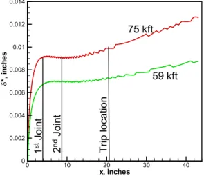
Subsequent to this calculation, the displacement thicknesses at 75 and 59 kft were recalculated using conditions from a revised trajectory including updated weights and wall temperatures. Figure 13 shows that at 75 and 59 kft the displacement thicknesses are approximately 0.01 in. and 0.00725 in. respectively. These values correspond to k/δ* values of roughly 8 and 11. These values are significantly larger than the k/δ* = 3.2 design criteria and thus are almost sure to result in a turbulent boundary layer through the test window.
x, inches δ∗ ,i n ch es 0 10 20 30 40 0 0.005 0.01 0.015 0.02 0.025 0.03
Figure 12: Displacement thickness for HIFiRE flight, 111 kft. Point is displacement thickness at trip location
x, inches δ *, in ch e s 0 10 20 30 40 0 0.002 0.004 0.006 0.008 0.01 0.012 0.014 59 kft (18 km) 75 kft (23 km) T rip loc ation 2 nd Jo in t 1 stJo in t 59 kft 75 kft x, inches δ *, in ch e s 0 10 20 30 40 0 0.002 0.004 0.006 0.008 0.01 0.012 0.014 59 kft (18 km) 75 kft (23 km) T rip loc ation 2 nd Jo in t 1 stJo in t 59 kft 75 kft
Figure 13: Displacement thickness for revised HIFiRE flight trajectories
Allowable Roughness Height
The flight vehicle forecone buildup will consist of a refractory metal tip 3.94 in. long (either tungsten or molybdenum) followed by a steel frustum 4.72 in. long, followed by the aluminum cone body. An allowable roughness limit of 3.15x10⁻³ in. (Ref. 19) on the laminar side of the forecone of was imposed by the correlation in
Ref. 18. This roughness limit was re-investigated based on the incipient trip criteria determined from the LaRC results, k/δ*=1.2. The displacement thickness distribution along the forecone for the revised HIFiRE trajectory is shown in Fig. 13 at altitudes of 75 and 59 kft. The most upstream nosetip joint, x=3.94 in., for 59kft is the location/altitude combination that would result in the smallest allowable surface discontinuity to ensure smooth-body transition on the laminar, non-tripped, side of the forecone. This location/altitude combination has a displacement thickness of approximately 0.00625 in. resulting in an allowable roughness of k = 7.5x10⁻³ in. which is
over twice the limit imposed based on initial analysis. Given the uncertainty in roughness correlations it was deemed prudent to retain the original, more restrictive roughness limit of 3.15x10⁻³ in.
Since the flight vehicle forecone sections are comprised of dissimilar metals, differences in flight surface temperatures and coefficients of thermal expansion for these materials will result in different values of thermal expansion for each section. The temperatures and coefficients of thermal expansion are such that each piece will expand more than the material upstream of it. If the parts were sized to be flush at each joint at room temperature, a forward-facing step would occur when the parts heated. For this reason the parts will be dimensioned so that a backward-facing step occurs at room temperature for each joint. The height of the joint is determined so that the parts will be near flush at 59 kft. The joint sizing is shown in Table 2. The minimum and maximum cold steps are determined from the stackup of tolerances in the mating pieces. The thermal expansion range at 59 and 75 kft is the difference in part radius due to thermal expansion and reflects uncertainty in temperature and material properties. The worst-case steps at 59 and 75 kft represent a stackup of tolerances and thermal expansion uncertainties. The
0.0209 = k/3.2
worst case at 75 kft is a forward-facing step which would occur if thermal expansion is at the low range of expected values. Even so, the values are an order of magnitude less than the incipient roughness determined from the LaRC test. Likewise, the worst case at 59 kft is a backward-facing step which is an order of magnitude less than the allowable roughness. An additional margin of safety arises from the nature of the wind tunnel trip geometry versus the flight geometry. Roughness arising from joints on the flight vehicle will generally be backward facing steps. The “pizza box” trip geometry is a more effective trip than a backward facing step, so its incipient trip height should be less than that for a backward facing step.
Table 2: Steps at nose joint locations on flight vehicle BFS – Backward Facing Step, FFS – Forward Facing Step
Joint x-Location 3.94 in 8.66 in
Min Cold Step 0.0039 0.0024
Max Cold Step 0.0053 0.0037
Thermal Expansion 59 kft 0.0028-0.0039 0.0016-0.0024 Thermal Expansion 75 kft 0.0035-0.0047 0.0020-0.0028 59 kft Worst Case Step 0.0026 BFS 0.0022 BFS 75 kft Worst Case Step -0.00079 FFS -0.00039 FFS
D. Effect of Flare Duct
The HIFiRE Flight 1 payload includes a duct on the flare surface to be used for an optical mass capture experiment. Two of the full vehicle wind tunnel models were fabricated with a duct on the flare and one was not. The purpose of the duct for the wind tunnel test was to determine the effect the duct would have on the shock-boundary layer interaction. During this test, heating images of the full models with and without the flare were taken. Additionally, for a limited set of conditions, the camera was focused on the flare region in order to give a more detailed view of the surface heating during the test. Testing was completed with and without the boundary layer trips in order to determine the effects of laminar versus turbulent conditions on the cone. Figure 14 shows the heating for the full vehicle model with the 33-deg flare with and without the boundary layer trip and with and without the duct present. Figure 15 shows global heating images of the flare region for the 33-deg flare model, and Fig. 16 shows the data, focused on the duct region. Both sets of data are taken along the centerline of the model and through the duct.
0.00 0.02 0.04 0.06 0.08 0.10 0.12 0.14 0 0.1 0.2 0.3 0.4 0.5 0.6 0.7 0.8 0.9 1 x/L h/ href no duct, no trip no duct, single trip duct, no trip duct, single trip
Mach 6
rn = 0.047 in
Re = 5.6x10⁶/ft
α = 0 deg
33-deg flare angle
(a) (b)
Figure 15: Global phosphor thermography images of the flare region, no trip, Re = 5.6x10⁶/ft, r
n = 0.047 in., 33-deg
flare angle, AoA = 0 deg; (a) without the duct; (b) with the duct
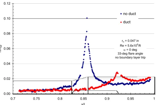
0.00 0.02 0.04 0.06 0.08 0.10 0.12 0.7 0.75 0.8 0.85 0.9 0.95 1 x/L h/ hre f no duct duct rn = 0.047 in Re = 5.6x10⁶/ft α = 0 deg
33-deg flare angle no boundary layer trip
Figure 16: Effect of the flare duct on the 33-deg Flare Angle Model, focused on flare region
There are two main conclusions that can be drawn about the effects of the flare duct. The first is that the large spike in heating associated with the flare angle (whether 33- or 37-deg) is reduced. This reduction in peak heating is due to the removal of the sharper compression surface associated with the flare. The duct presents a much less severe compression surface. Heating rates on the models without the duct have peaks two or more times higher than those with the duct. The second observation is that the duct causes a slight decrease in the heating on the cylinder just prior to the start of the flare, as compared to the heating rates without the duct. This reduction in heating is shown in both of the plots of focused data and is most likely due to the effects of flow separation prior to the start of the flare.13 The duct removes the sharp compression surface associated with the flare surface. The presence of the
duct does not affect the heating well downstream on the final cylinder.
E. Effect of Flare Angle
Two flare angles were used for this test series, 33-deg and 37-deg, with the 33-deg flare angle configuration designated as the primary flight test configuration. The 33 deg flare model was chosen as the flight configuration based on tests at the Calspan-University of Buffalo Research Center.20 These tests showed that the 33-deg flare
provided a turbulent separated region large enough to resolve experimentally, yet still reattached on the flare face. For the purpose of the work described in this paper, both the 33- and 37-deg flare angle models were tested with the duct (Fig. 17). The two flare angles were compared at a Reynolds number of 5.6x10⁶/ft at 0 deg AoA with and
without a single boundary layer trip. Comparisons are shown in Fig. 17 for the full vehicle and in Fig. 18 for runs focused on the flare.
0.00 0.02 0.04 0.06 0.08 0.10 0.12 0.14 0 0.1 0.2 0.3 0.4 0.5 0.6 0.7 0.8 0.9 1 x/L h/h ref
33 deg flare, no trip 37 deg flare, no trip 33 deg flare, single trip 37 deg flare, single trip
Mach 6
rn = 0.047 in
Re = 5.6x10⁶/ft
α = 0 deg
Figure 17: Effect of the flare angle
As shown in Fig. 17, there was very little effect of the flare angle on the heating for the vehicle. Heating rates before and after the flare were similar for the two flare angles. Fig. 18 additionally shows that each of the heating peaks, with and without the boundary layer trips, was slightly higher for the 37-deg flare angle model. Despite the 37-deg flare angle model having a more severe compression surface, there was no significant effect of the flare angle over this range. There was no significant effect of the variation of the flare angle on the heating of the HIFiRE vehicle with regards to the duct.
0.00 0.02 0.04 0.06 0.08 0.10 0.12 0.14 0.7 0.75 0.8 0.85 0.9 0.95 1 x/L h/ href
33 deg flare, no trip 37 deg flare, no trip 33 deg flare, trip array 37 deg flare, trip array
Mach 6
rn = 0.047 in
Re = 5.6x10⁶/ft
α = 0 deg
Figure 18: Effect of the flare angle, focused on flare region
IV. Concluding Remarks
The HIFiRE Flight 1 payload was assessed in the Langley Research Center’s 20-Inch Mach 6 Air Tunnel. The primary objective of this test was to determine the size and location of the boundary layer trip that will be incorporated onto the flight vehicle. In order to accomplish this, global heat transfer images were obtained for unit Reynolds numbers of 2.1x10⁶/ft to 5.6x10⁶/ft and angles of attack of -5 to +5 deg which were conditions pertinent to
the flight. A single boundary layer trip will be used on one side of the flight vehicle to ensure at least a portion of the vehicle is turbulent prior to breakup. The other side will be allowed to transition to turbulent naturally. The wind tunnel model reflected this trip configuration. Heating data demonstrated that the boundary layer trip height was able to generate fully turbulent heating rates. In order to ensure that the turbulent wedge from the boundary layer trip on the flight vehicle would not wash onto the other side and contaminate the laminar surface of the flight vehicle at angle of attack, the flight boundary layer trip was moved aft of the position that was used for the wind tunnel test. Additionally, the incipient trip height was determined in order to ensure that the joints on the flight vehicle would not cause the flow to transition to turbulent on the laminar side. The heating rates obtained using the global phosphor thermography technique were compared to predictions obtained using LAURA and matched very well for the forecone models at both laminar and turbulent heating rates.
Additional experimental objectives of the wind tunnel test were to investigate the effect of the flare angle of the full-vehicle configuration and determine the effects of a duct in the flare for use in an optical mass capture experiment. It was determined that a change in the flare angle has a minor effect on the peak heating, as expected, due to the change in the compression surface. Peak heating was higher for the 37-deg flare. Heating images also revealed a small separation region where the flare does not have the duct, but this separation region does not feed forward enough to affect the cone portion of the model. The separation region therefore does not affect the turbulent heating data associated with the primary goal of the experiment, to obtain turbulent heating data on a flight vehicle.
Acknowledgments
The authors would like to thank the following people for their contributions to the project: Gary Wainwright, Mike Powers, Mark Griffith, Ed Covington and Pete Veneris for their assistance in model design, fabrication and preparation; Grace Gleason, Harry Stotler, and Rhonda Mills for wind tunnel support; Kevin Hollingsworth and Teck-Sen Kwa for data acquisition assistance; Vincent Zoby for assistance in data interpretation and understanding; Christopher Alba and Heath Johnson for their detailed computations of the laminar boundary layer that were used to scale the trip heights. Without their help, these tests would not have been possible.
References
1 Buck, G. M., Powers, M. A., Griffith, M. S., Hopkins, J. W., Veneris, P. H., and Kuykendoll, K. A., "Fabrication of 0.0075-Scale Orbiter Phosphor Thermography Test Models for Shuttle RTF Aeroheating Studies," NASA TM-2006-214507, May 2006.
2 Micol, J. R., "Langley aerothermodynamics facilities complex: enhancements and testing capabilities," AIAA-98-0147, Jan 1998.
3 Buck, G. M., “Automated thermal mapping techniques using chromatic image analysis," NASA TM-101554, April 1989.
4 Merski, N. R., "Reduction and analysis of phosphor thermography data with iheat software package," AIAA-98-0712, Jan 1998.
5 Merski, N. R., "Global aeroheating wind-tunnel measurements using improved two-color phosphor thermography model," Journal of Spacecraft and Rockets, Vol., 36, No., 2, 1998, pp. 160-170.
6 Fay, J. A., and Riddell, F. R., "Theory of Stagnation Point Heat Transfer in Dissociated Air," Journal of Aeronautical Sciences, Vol. 25, No. 2, 1958, pp. 73-85.
7 Gnoffo, P. A. "An Upwind-Biased, Point-Implicit Relaxation Algorithm for Viscous Compressible Perfect Gas Flows," NASA TP-2953, Feb 1990.
8 Cheatwood, F. M., Gnoffo, P. A. "User's Manual for the Langley Aerothermodynamic Upwind Relaxation Algorithm (LAURA)," NASA TM-4674, April 1996
9 Horvath, T. J., Berry, S. A., Hollis, B. R., Chang, C., and Singer, B. A., "Boundary Layer Transition on Slender Cone in Conventional and Low Disturbance Mach 6 Wind Tunnels," AIAA-2002-2743, June 2002.
10 Johnson, H. B., Alba, C. R., Candler, G. V., MacLean, M., Wadhams, T, and Holden, M. “Boundary Layer Stability Analysis to Support the HIFiRE Transition Experiment,” AIAA-2007-0311, January 2007.
11 Berry, S. A., Hamilton, H. H., "Discrete Roughness Effects on Shuttle Orbiter at Mach 6," AIAA-2002-2744. June 2002.
12 Berry, S. A., Horvath, T. J., Roback, V. E., and Williams Jr., G. B., "Results of Aerothermodynamic and Boundary Layer Transition Testing of the 0.0361-Scale X-38 (Rev 3.1) Vehicle in the NASA Langley 20-Inch Mach 6 Tunnel," NASA TM-112857, September 1997.
13 Alba, C., Johnson, H. and Candler, G., “Boundary Layer Stability Calculations of the HIFiRE Flight 1 Vehicle in the LaRC 20- Inch Mach 6 Air Tunnel,” AIAA-2008-0505, January 2008
14 Berry, S. A., and Horvath, T. J., “Discrete Roughness Transition for Hypersonic Flight Vehicles,” AIAA-2007-0307, January 2007.
15 Schneider, S. P., “Effects of Roughness on Hypersonic Boundary Layer Transition,” AIAA-2007-0305, January 2007.
16 Stainback, C. P., “Effect of Unit Reynolds Number, Nose Bluntness, Angle of Attack, and Roughness on Transition on a 5o Half-Angle Cone at Mach 8,” NASA TN D-4961, January 1969.
17 Reda, D. C., “Review and Synthesis of Roughness-Dominated Transition Correlations for Reentry Applications,” Journal of Spacecraft and Rockets, vol. 39, no. 2, March-April 2002, pp. 161-167. 18 Berry, S. A., Bouslog, S. A., Brauckmann, G. J., and Caram, J. M., “Shuttle Orbiter Experimental
Boundary-Layer Transition Results with Isolated Roughness,” AIAA Journal of Spacecraft and Rockets, vol. 35, no. 3, May-June 1998, pp. 241-248.
19 Kimmel, R. L., Adamczak, D., Gaitonde, D., Rougeux, A., Hayes, J. R., "HIFiRE-1 Boundary Layer Transition Experiment Design," AIAA-2007-0534, January 2007.
20 Wadhams, T. P., MacLean, M. G., Holden, M.S., and Mundy, E., “Pre-Flight Ground Testing of the Full-Scale FRESH FX-1 at Fully Duplicated Flight Conditions,” AIAA- 2007-4488, June 2007