The flow structure behind vortex generators embedded in a decelerating turbulent boundary layer

To link to this article

:

http://dx.doi.org/10.1080/14685240903273881

URL:

http://www.tandfonline.com/doi/abs/10.1080/14685240903273881

This is an author-deposited version published in: http://oatao.univ-toulouse.fr/

Eprints ID: 6326

To cite this version:

Cathalifaud, Patricia and Godard, Gilles and Braud, Caroline and

Stanislas, Michel

The flow structure behind vortex generators embedded

in a decelerating turbulent boundary layer.

(2009) Journal of Turbulence,

vol. 10 (n° 42). pp. 1-37. ISSN 1468-5248

Open Archive Toulouse Archive Ouverte (OATAO)

OATAO is an open access repository that collects the work of Toulouse researchers

and makes it freely available over the web where possible.

Any correspondence concerning this service should be sent to the repository

administrator:

[email protected]

The flow structure behind vortex generators embedded in a

decelerating turbulent boundary layer

P. Cathalifauda_{, G. Godard}b_{, C. Braud}c_{and M. Stanislas}c∗

a_{Institut de M´ecanique des Fluides (UMR 5502), UPS, Universite Paul Sabatier, 18, route de}

Narbonne, 31062 Toulouse C´edex, France;b_{CORIA (UMR 6614), CNRS, Site Universitaire du}

Madrillet, 6801 Saint Etienne de Rouvray C´edex, France;c_{Laboratoire de M´ecanique de Lille}

(UMR 8107), EC Lille, CNRS, Boulevard Paul Langevin, Cit´e Scientifique, 59655 Villeneuve d’Ascq C´edex, France

The objective of the present work is to analyse the behaviour of a turbulent decelerating boundary layer under the effect of both passive and active jets vortex generators (VGs). The stereo PIV database of Godard and Stanislas [1, 2] obtained in an adverse pressure gradient boundary layer is used for this study. After presenting the effect on the mean velocity field and the turbulent kinetic energy, the line of analysis is extended with two points spatial correlations and vortex detection in instantaneous velocity fields. It is shown that the actuators concentrate the boundary layer turbulence in the region of upward motion of the flow, and segregate the near-wall streamwise vortices of the boundary layer based on their vorticity sign.

Keywords: flow control, vortex generators, turbulent boundary layer, adverse pressure

gradient, PIV, coherent structures

1. Introduction

Delaying or preventing turbulent boundary layer (TBL) separation in aeronautic applications (during landing or manoeuvre of an aircraft for example) leads to enhance the lift to drag ratio and thus to fuel saving and reduction of the emitted pollution. It allows also to extend the flight envelop of an aircraft. For that purpose many actuator types were explored in the last decades over many flow configurations (flat plates, ramps, bumps, ducts, airfoils, wind turbines, etc.) [3].

Among the actuators used for that purpose, the vortex generators (VGs) were found efficient to reduce and sometimes even suppress the separated region [4]. These devices generate a streamwise vortex structure which can entrain high-momentum fluid towards the wall, hence energising the TBL, increasing quantities such as wall shear stress, tur-bulence intensities, momentum transfer, etc. and delaying separation. The optimal device would produce streamwise vortices just strong enough to overcome the separation without persisting within the boundary layer once the flow control objective is reached. It can be either passive or active. The resulting streamwise vortices have been subjected to many studies which helped to characterise the optimal actuator parameters and the resulting mean organisation. However, too few studies were performed on the flow re-organisation due to the difficulty to get a sufficient spatial resolution in the TBL.

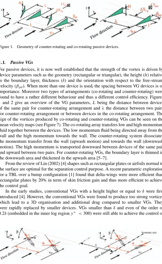
Figure 1. Geometry of counter-rotating and co-rotating passive devices.

1.1. Passive VGs

For passive devices, it is now well established that the strength of the vortex is driven by device parameters such as the geometry (rectangular or triangular), the height (h) relative to the boundary layer, thickness (δ) and the orientation with respect to the free-stream velocity (βpd). When more than one device is used, the spacing between VG devices is of

importance. Moreover two types of arrangements (co-rotating and counter-rotating) were found to have a rather different behaviour and thus a different control efficiency. Figures 1 and 2 give an overview of the VG parameters,L being the distance between devices of the same pair for counter-rotating arrangement andλ the distance between two pairs for counter-rotating arrangement or between devices in the co-rotating arrangement. The sign of the vortices produced by co-rotating and counter-rotating VGs can be seen on the mean velocity maps (see Figure 7). The co-rotating array transfers low and high momentum fluid together between the devices. The low momentum fluid being directed away from the wall and the high momentum towards the wall. The counter-rotating system dissociates the momentum transfer from the wall (upwash motion) and towards the wall (downwash motion). The high momentum is transported downward between devices of the same pair and upward between two pairs. For counter-rotating VGs, the boundary layer is thinned in the downwash area and thickened in the upwash area [5–7].

From the review of Lin (2002) [4] shapes such as rectangular plates or airfoils normal to the surface are optimal for the separation control purpose. A recent parametric exploration for a TBL over a bump configuration [1] found that delta-wings were more efficient than rectangular plates by 20% in term of skin friction gain and thus more efficient to achieve the control goal.

In the early studies, conventional VGs with a height higher or equal to δ were first introduced [4]. However, the conventional VGs were found to produce too strong vortices which lead to a 3D organisation and additional drag compared to smaller VGs. They were rapidly replaced by smaller devices. VGs smaller than δ and even of the order of 0.2δ(embedded in the inner log regiony+ <300) were still able to achieve the control of

separated flows with less associated drag than conventional VGs. Off course, the streamwise lifetime of the corresponding vortices is smaller. Lin (2002) [4] suggests that these devices should be applied close to the separation region when it is relatively fixed.

The skew angle to the free streamβpd determines the vortex strength and lateral path

[8]. Tilmann et al. (2002) found that increasing βpd generally increases the circulation

and thus the control goal effectiveness. However, Godard and Stanislas (2006) [1] found by decreasing βpd from 23◦ to 13◦ that the vortices can be linearly strengthened up.

Actually, an optimum angle of attack exists which is found equal toβpb=18◦by Godard

and Stanislas (2006) [1] for a bump configuration. In addition, a rapid decay of the peak vorticity downstream of the VG is observed, regardless ofβpb[1, 4, 7, 8].

For a defined flow configuration (TBL over a bump, ramp, airfoil, etc.), once the optimal βpbis found, there exit an optimal number of devices in the spanwise direction depending

on the spanwise arrangement of the VGs and the available transverse space. Godard and Stanislas [1], by measuring the downstream wall shear stress between devices of the same pair and between two pairs of counter-rotating VGs, could perform a parametric study. They found two effects when increasing the height of the device and thus the vortex circulation. In between a pair of counter-rotating VGs, the gain in term of skin friction saturates over h=0.2δ, whereas it still increases overh=0.4δ between devices of the same pair. Actually, the distance between devices, for both co-rotating or counter-rotating arrangement, is of major importance [1, 4, 5, 7]. For counter-rotating arrangements, contrary to the co-rotating ones, decreasing the transverse distance between devices was found to blow-up the vortices. On the contrary, increasing too much the spacing between devices decreases the effectiveness locally [1, 5]. Departing from a non-equidistant state (λ/L=4) Angele et al. (2005) [5] recently found, from extensive SPIV measurements, that the centres of the vortices move downstream towards an equidistant state and remain submerged in the TBL, contrary to the non-viscous theory. Therefore, the optimal spacing should be close to the equidistant state and the position of the VGs should be far enough upstream of the separation line in order for the vortices to become equidistant and to avoid back-flow in between actuators [5]. Moreover, it should be close enough to the separation line to avoid additional drag from the downstream travelling of the streamwise vortices. The optimal streamwise distance between the vortex generators line and the minimum skin friction station (or the separation line)Xvgis experienced to beXvg/ h < 100, but depending

on the flow configuration (bump, ramp, airfoil, duct, etc.) [1, 4].

Note that most of the studies did not perform parametric investigations which are time consuming. The most investigated parameter is the heighthof the device.

Many fundamental studies were performed to analyse the organisation of the streamwise vortices produced by VGs embedded in a zero-pressure gradient (ZPG) TBL (among others [7, 9–13]). Recent studies are addressing more realistic configurations which are streamwise vortices embedded in an APG-TBL with or without separation ([1, 5, 14] among others). Indeed the flow in which the VG is embedded influences the dynamics of the produce vortices. Viscous diffusion causes the vortices to grow, the swirling velocity component to decrease and the BL to develop towards a 2D state [5]. The adverse pressure gradient is found to promote interactions between vortices hence decreasing the control effectiveness [4]. Therefore, depending on the flow configuration (flat plate within an APG, ramp, bump, etc.) the optimal parameters vary. The main flow influence is still under investigation.

Logdberg et al. (2009) [7] have recently analysed the mean vortex path of longitudinal vortices produced by rectangular plates devices (or vane types) within a ZPG-TBL by means of flow visualisation and hot-wire measurements. This mean path is determined from the

maximum positive value of the mean velocity gradient tensor second invariant at different streamwise positions. For a counter-rotating array configuration of VGs, the vortices from the same pair first move away from each others. Thus, they move closer to the neighbouring vortex pair and eventually form a new counter-rotating pair with a common flow. Then the vortices move away from the wall. From the authors, this is due to the induced velocity in the upwash motion that tends to lift the vortices. Finally, they move again towards each other, closer to the equidistant-state. The authors attribute this last peculiar hook-like motion to the vortex growth and the limited space inside the boundary layer due to the neighbouring vortices. The maximum mean vortex radius is estimated to beλ/4 which implies that the mean vortex centre path is within a circle defined as followed:y/ h=2.08;z/λ= ±0.25. Angele et al. [5] and Logdberg [14] also provide a useful rough evaluation of the vortex circulation,γ =2khUvg/λ, wherekis a coefficient that depends on the device used

(k=0.6 for vane-type VG in a ZPG configuration), andUvgis the streamwise velocity at

the tip of the device. However, this does not include the influence of the skew angle and the cross-flow organisation.

The development of SPIV measurements led to further understanding of the VGs/TBL interaction. Angele et al. (2005) [5] have recently analysed the VGs/APG-TBL interaction in terms of turbulent properties. In that study the APG induce a small separation area. They found that most of the turbulence production is locally governed by one of the gradients dU/dyordU/dzfrom the S-shape profile of the streamwise velocity in the x-y plane and the mushroom shape of the streamwise velocity in the y-z plane. In span, between vortices, the spanwise gradient involves significant levels of turbulence production, however the flow is overall more isotropic.

1.2. Active VGs

Passive devices were rapidly replaced by active ones which can be turned off when not necessary in order to avoid additional drag (i.e. during cruise flight of an aircraft for instance). Many active device types were then developed for which, depending on the control source used, the control is of different nature (acoustic actuators, plasma actuators, fluidic actuators, etc.). Moreover, within fluidic actuators, one can distinguish synthetic jets devices also called Zero-Net Mass Flux [15–17] and pulsed-jet actuators [18, 19]. Indeed, for synthetic jets, contrary to pulsed-jets, there exists a suction phase. Moreover, different jet orifice shapes, orientations and operating parameters (jet oriented normal to the wall, high or low pulsating frequency, low or high velocity ratios VR between the jet exit velocity and the local free stream velocity, etc.) are used, which lead to different types of control. For instance, Greenblatt and Wygnansky [20] talk about coherent structures enhancement also called hydrodynamic control. For this control type, a low VR and a pulsating frequency adapted to the natural shedding frequency of the coherent structures is thought to be efficient. On the other hand, Raman et al. [21] are dealing with the small turbulent structures; acting one these scales is thought to allow to modify the large scale organisation more efficiently than the hydrodynamic control (no development of another dominant harmonic).

The present work is focused on control studies using fluidic actuators with addition of mass to generate streamwise vortices (also called pulsed-jets actuators or pneumatic vortex generators).

In continuous mode of the actuator, the streamwise evolution of the produced vortices by a single active device has been extensively analysed in ZPG configurations ([8, 22, 23] among others). The circulation and the associated strength of the vortex is modified by

parameters such as the ratio between the jet exit velocity and the local free stream velocity VR, the actuator pitchβand skewαangles and the orifice shape (see Figure 2 for notations). Contrary to passive devices, the arrangement may influence significantly the produced jet, leading to additional parameters dependency. Indeed, as highlighted in Peterson et al. [24] and Warsop et al. [25], a separation occurs within the tube (or hole) due to the supply channel flow shear at the leading or trailing edge of the hole. Warsop et al. [25] found this phenomena responsible of pressure losses up to 40% at the exit, whereas Peterson and Plesniak [24] show that for low aspect ratio of the orifice exit (less than unity), the trajectory and the spanwise spreading of the exit jet can be modified depending on the sign of the ‘supply channel-inhole flow”.

Peterson and Plesniak [24] performed an extensive PIV analysis of streamwise vortices embedded in a TBL (flat plate configuration) for round jet actuators placed perpendicular to the wall. Measurements where taken in the plenum chamber and the exit hole and immediately downstream the hole. Even if the exit hole was perpendicular to the wall, this gives insight in the vortex formation mechanism. A single jet perpendicular to a wall gives rise to a pair of counter-rotating streamwise vortices, whereas two inclined jets are needed to get a qualitatively equivalent vortex pair. The origin of the remaining counter-rotating vortex pair from the jet/free stream interaction is explained by the high shear from the jet edges which induces a roll-up of the boundary layer flow. The shear is more important at the trailing edge of the hole due to bending of the jet. Behind the jet, a true wake region does not develop, but rather the action of the counter-rotating vortex pair draws the fluid away from the wall which creates a recirculation region of low velocity immediately downstream of the jet along the x-axis. When the blowing ratio increases, the jet lifts from the wall and the recirculating region is significantly reduced. Additionally, large separations occurs within the exit hole of the jet which affects the following development of the two counter-rotating vortices immediately downstream the hole, when the aspect ratio of the exit hole is short (lower than 1). For instance, for a flow in the supply channel pointing in the same direction as the main flow, the counter-rotating vortices from the jet/free stream interaction are enhanced, up to 35% compared to supply channel pointing in the opposite direction to the main flow, and thus penetrates further into the TBL. Moreover, the spanwise spreading slightly decreases, when compared to supply channel pointing in the direction opposite to the main flow.

When the jet has an angle to the wall (pitch and/or skew angle), two counter-rotating vortices are initially created just downstream of the device which evolves rapidly into a single coherent vortex of one sign accompanied by a much smaller and weaker region of circulation of the opposite sign near the wall [8]. The performances increase with VR and the effect is persistent far downstream from the injection (Xvg/=200 orXvg/δ =40).

For passive VGs, the primary vortex continues to move laterally in the direction of the vane skew, while for active VGs the path of the primary vortex is driven by VR. Consequently, too high jet exit velocity (VR) can blow the vortices out of the TBL, where it is overwhelmed by the free-stream momentum and quickly dissipates, hence reducing the control effectiveness [8]. For single VGs embedded in the TBL, the vortices are similar (at least qualitatively) to the ones from passive VGs [8, 22].

Different VGs arrangements were also investigated [2]. The sign of the produced vor-tices from co-rotating (CO) and counter-rotating (CT) arrangements is found similar to the passive ones. The CT active VGs are found to produce similar vortices as passive ones in the same arrangement. On the contrary, CO-active VGs merge more rapidly than passive ones and thus they dissipate more rapidly. The optimal distance between devices was found 10-times smaller than for passive devices but with a higher achievable skin friction gain. For

CT actuators, the skin friction gain is proportional to VR with little skin friction gain over VR = 3.1 for a TBL over a bump configuration without separation [2]. Hence, an optimal VR exists over which the vortices may be bleed out of the TBL which wasn’t observed by the authors. Logdberg [14] found that the necessary VR to achieve the control goal varies little with APG. With the assumption that for the same effectiveness criteria, the circulation is identical for both active and passive devices, a rough evaluation of the circulationγ for active devices was performed. Also,γ =1.0 to 1.5 was found enough to overcome the small separation in all three APG tested. These authors also suggest that an increase of the number of jets should be preferred to improve further the control effectiveness rather than an increase of VR (in the limit of the optimal spacing). For low VR (<4.7) and depending on the main flow configuration, the optimal skew angle is found between 45◦ and 90◦ [2, 26, 23].

The use of active VGs in the pulsed mode enables to decrease further the mass flow consumption of the actuator. Indeed, in the pulsed mode the pulsating frequency and the Duty Cycle (DC) can be tuned so that successive streamwise vortex segments can merge downstream, producing quasi-continuous streamwise vortices with less mass flow rate than the steady case [8, 19]. Also, depending on the main flow configuration (i.e. attached or separated TBL over a ramp, bump, etc.) and the actuator-jet strength (VR), the jet penetration may be modified by the pulsating frequency. Moreover, Tilmann [8] observed that pulsating the jet always generates a stronger primary vortex independently to the width of the DC. More recently, Ortmann and Kaehler, and Kostas et al. [18, 19] found a significant improvement of the control effectiveness during the first millisecond of the activation/deactivation of the actuator which was related to unsteady oscillations of the jet exit during these phases and subsequent modulation of the primary vortex strength. These oscillations were later found to be related to a wave propagation phenomena in the feeding tube of the actuator [27]. The exit jet from the fluid VG was analysed in detailed by [28]. However, this is beyond the scope of this paper which treats only the continuous mode of operation of active VGs.

These studies allow to conclude on the effectiveness of the actuator and on the mean organisation of the resulting TBL/VGs interaction. However, too little attention was paid to the TBL reorganisation behind VGs actuators. This is mainly due to the difficulty to get a good spatial resolution inside the TBL. In the present facility, the TBL is 10-times scaled-up compared to typical experimental facilities which enables to performed a more detailed analysis of the interaction between the APG-TBL and passive or active VGs. This is done using stereo PIV in different planes normal to the flow, downstream of the actuators. The mean flow and turbulent kinetic energy distributions are first characterised. Then a vortex detection analysis is performed on the instantaneous stereo PIV measurements (see Tables 1 and 2). This gives a better insight into the reorganisation of the main flow turbulence in the presence of streamwise vortices.

Parametric studies of different kinds of vortex generators were performed by Bernard et al. [29], Godard and Stanislas [1] and Godard and Stanislas [2] as part of two European projects called AEROMEMS and AEROMEMS II. The objectives were to optimise different actuator systems in order to control separation on an airfoil or a wind flap using Micro Electro-Mechanical Systems (MEMS) technology. Since such systems have very small scales, an enlargement of the scale of the phenomenon was decided to overcome the problem of spatial resolution. A stereoscopic PIV experiment was also performed by Godard and Stanislas [1] and Godard et al [32, 33].

In Section 2, the experiments performed to obtain the present database are described. In Section 3, one point statistical analysis are presented (mean velocity and turbulent kinetic

Figure 3. Front view of the TBL wind tunnel.

energy). In Section 4, the spatial correlation is analysed. In Section 5, the vortex detection method and the corresponding results are shown. Finally, a general conclusion is provided.

2. Description of the database

The facility used to acquire the database has the particularity to enable a TBL withδup to 300 mm, fully developed in the test section and characterised in the flat plate configuration by [30]. Some years ago, a bump was added within this TBL. This configuration represents the non-actuated case. A detailed analysis of this bump flow was performed by Bernard et al. [31]. Later, Godard et al. [1, 2, 32] analysed the effectiveness of different VG devices from an extensive parametric study. Gain in terms of shear stress measurements were compared and led to optimal configurations. SPIV measurements were then performed on these configurations and briefly described [33]. The same SPIV database is used in the present analysis with optimal parameters of the devices. To help the reader, some information concerning the database is recalled in this section.

2.1. The wind tunnel

Figure 3 is a front view of the boundary layer wind tunnel used. It is 20 m long. The last 5 m are transparent on all sides to allow the use of optical methods, and the test section is 1×2 m2. The free stream velocity for the present database was set at 10 m/s. The wind tunnel was used in closed loop to allow the use of smoke. The wind tunnel velocity is computer controlled by a PC within±0.01%). The boundary layer under study develops on the lower wall. It is tripped at the entrance of the tunnel by a grid laid on the floor. The origin of the coordinate system is placed in the middle of the lower wall at the entrance of the tunnel. Thex-axis is parallel to the wall and to the flow, they-axis is normal to the wall, the reference frame is direct. At the beginning of the bump,x= 15.5 m, the boundary layer thickness isδ=300 mm.

2.2. The bump

The objective of the AEROMEMS projet was to design a bump with a pressure gradient representative of what happens on the suction side of an airfoil at moderate angle of attack and to approach separation without reaching it in order to prevent the flow to become 3D. The coordinates of the bump can be found in Bernard et al. [31]. The flow in the first half of the bump strongly accelerates with a rapid variation of the pressure gradient magnitude. Atx = 17 m, the sign of the pressure gradient changes and its variation becomes more

Figure 4. Distribution of the pressure coefficient over the bump.

progressive in order to avoid separation (see Figures 4 and 5). The skin friction decreases rapidly and reaches a minimum aroundxcf min= 18.58 m.

2.3. The actuators

The device parameters were taken from the optimal configuration found by [1] and [2] for the same base flow. If the optimal streamwise location of the passive device was found, it was not possible, due to mechanical constraints, to place jets VGs at the same station. Active VGs were placed 0.45 m downstream of the best passive device location. However, in order to compare the active and passive actuation, measurements were also performed for a passive vortex generators array (PAb) at the same location as the round jetsXd =17.55 m.

The VGs used are:

r

(1) a spanwise row of counter-rotating VGs at Xd =17.10 m (optimal streamwise

location) (PA)

(2) a spanwise row of counter-rotating VGs atXd =17.55 m (PAb)

Table 1. Parameters for the passive vortex generator actuators (PA) in the counter-rotating arrangement (h=26 mm).

Type δ(mm) Xd(m) h/δ l/ h L/ h λ/ h βpd XV G/ h Nj

PA 70 17.10 0.37 2 2.5 6 18 57 22

PAb 165 17.55 0.158 2 2.5 6 18 57 22

r

(1) a unique pair of counter-rotating VGs (CT) (2) a spanwise row of co-rotating VGs (CO)

The parameters of the VG used are summarised in Tables 1 and 2:δ is the boundary thickness without actuation at the device location,Xd is the position of the devices in the

streamwise direction (see Figures 1 and 2), h is the height of the passive devices, l/ h is the aspect ratio,λ is the transverse spacing between two devices (of the same pair in counter-rotating configurations),Lis the transverse spacing between two counter-rotating pairs,βpd is the orientation relative to the free-stream velocity,XV G=Xcf min−Xd is

the distance between the location of the minimum friction coefficient (without actuation) and the position of the devices in the streamwise direction,Nj is the number of individual

devices and VR the ratio between the jet velocity and the local free stream velocity of the base flow. The fluidic actuators are fed from a reservoir with a tube length of 200 mm and they are operating at constant pressure.

2.4. SPIV measurements

A standard stereo PIV set-up was used in the configuration shown in Figure 6. It basically consists of two Nd:Yag laser cavities, each of them producing about 250 mJ per pulse at 12.5 Hz (nominal pulse frequency). The pulse duration is 5 ns. The light sheet optics consist of two lenses: one spherical to adjust the light sheet thickness (about 1 mm) and one cylindrical lens to fix the light sheet width (about 400 mm). As the main flow is going through the light sheet, a small separation, of the order of 0.5 mm, is set between the first and the second light sheets to allow a larger dynamic range.

To record the images, two PCO sensicam cameras from lavision were set on both sides of the wind tunnel in a Sheimpflug configuration. They provide 1280×1024 pixels image pairs with 12 bits dynamic range. For the present experiments, Nikon lenses of focal length f =100 mm were used. The magnification was aroundM=0.14. With an aperture of 4, the diffraction spot size was of the order of 20µm. The Davis software and hardware from Lavision were used for recording. The calibration was performed by recording images of a plane target at three different positions around the light sheet. Measurements were

Table 2. Parameters for the active vortex generator actuators in the counter-rotating (CT) and in the co-rotating (CO) (=6 mm).

Type δ(mm) Xd(m) /δl L/ λ/ α-β XV G/δl Nj VR

CT 165 17.55 0.036 15 – 45-45 7.2 2 3.1

Figure 6. Scheme of the stereo PIV set-up used.

performed at three locations along the bump,Xpiv=17.67m, 18.09m, 18.57m. The

relative distanceXd =Xpiv−Xdis given in Table 3. The measurement planes are located

between the location of the actuators and the minimum of skin friction for VGs in their optimal configuration [1] and [2]. In other words, the VGs are still efficient in the last measurement plane, which is nearly at the minimum skin friction position. From now on these three stations will be respectively referred to as plane 1, plane 2 and plane 3. Note that for the PAb configuration only two downstream locations were recorded (Xd/ h=

21 andXd/ h=40).

The images from both cameras were processed with a standard multi-grid algorithm, with discrete window shifting and Gaussian peak fitting. The final interrogation window size was 32×32 pixels with 50% of overlap. The Soloff method with three calibrations planes was used to reconstruct the three velocity components in the plane of measurement. This was done using a home-made software.

At each station, 200 instantaneous velocity maps were recorded, corresponding to 800 images of 1280×1024pixels2. In the case of the counter-rotating arrangement (both passive and active), the images were centred successively on the downwash region (PAD, PADb and CTD configurations) or the upwash one (PAU and CTU configurations). We call downwash a region where the flow is directed towards the wall, and upwash a region where the flow is ejected from the wall.

Table 3. Location of the SPIV plane measurements relative to the location of the different devices (PA, PAb, CT and CO) withh=26 mm, =6 mm andδ as the boundary layer thickness at each location of the measurement plane.

PA PAb CT/CO

Plane Xpiv(m) δ(mm) Xd/δ Xd/ h Xd/δ Xd/ h Xd/δ Xd/

1 17.67 198 2.94 22 – – 0.63 20

2 18.09 315 3.92 38 2.17 21 2.17 90

3. One point statistical analysis 3.1. Mean velocity

3.1.1. Mean velocity maps

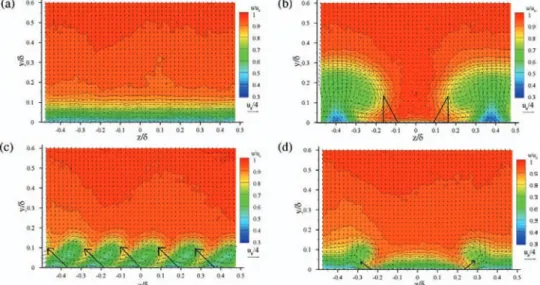
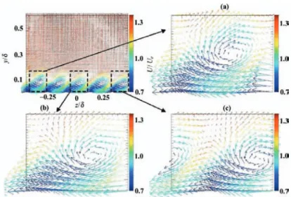
Figures 7 to 9 give the mean velocity maps obtained at the three streamwise stations (plane 1, plane 2 and plane 3) for the three types of device: passive actuators PA (or PAb) and active counter-rotating (CT) and co-rotating (CO) devices (see Table 3). The in-plane velocity is described by the in-plane vector components, while the colour coding gives the (main)out of plane component.

Plane 1

At the first streamwise location (Figure 7), which was selected to characterise the vorticies just after development, the flow without actuation (WAC case) is 2D and uniform in the spanwise direction. The strong gradient region near the wall, which is still quite thin at this station, is clearly visible from the rapid colour variation at the bottom part of the map. For the actuated cases, at this station which is very near to the jets actuators, the vortices are clearly detectable for all the devices tested.

For the passive devices in a counter-rotating arrangement (PAD case), the flow resulting from the device/BL interaction leads, as expected, to two streamwise counter-rotating vortices. The centres of the vortices are located around [y/δ=0.125;±z/δ=0.25] or [y/ h=1.9 ;±z/λ=0.32] which is in very good agreement with the location of the centres given by Logdberg [7]. In the middle of the field, a strong downwash region, induced by the two counter-rotating vortices is observed, associated with a strong streamwise velocity near the wall. At the edges of the PIV field of view, between the counter-rotating pairs, an upwash motion is observed coupled with a low streamwise velocity near the wall. Angele and Muhammad-Klingmann [5] have observed a similar inflection point configuration in the mean profiles, which is at the origin of a complex turbulent production process. As

Figure 7. Plane 1: WAC, PAD, CO and CTD. The black triangular in the PAD case represents the passive devices projected on the y-z plain. The Black arrows represents the jet direction from the active devices.

expected, the vortices produced by the PA actuators, which are located further upstream (Xd =17.10 m instead ofXd=17.55 m, see Table 3), are bigger in size than those due to

the active devices, for which the perturbed region is two-times smaller (beneathy/δ=0.2). For counter-rotating jets, a qualitative agreement is found with passive devices. The same signs of counter-rotating vortices are found with the centre closer to the wall [y/δ= 0.065;±z/δ=0.25] or [y/ h=0.5 ;±z/δ=0.25]. However, some differences are found. The mushroom-like shape is flatter than with passive devices which leads to a spreading of the structure in the transverse direction. Also, in between devices of the same pair, the streamwise velocity is weaker. This can be explained at first by the fact that in the CT case, the vortices are just developing in plane 1 while for the PA case they are fully established. Also only one pair of counter-rotating devices is used for the CT case whereas 11 pairs are used for the PA case. The second explanation is more plausible because these differences are retrieved in plane 2 where the actuators are this time at the same streamwise location.

For the co-rotating jets configuration, the flow shows a clear periodicityz/δ0.2 of co-rotating vortices which corresponds to the periodicity of the device arrangement λ/δ0.2. A low streamwise velocity is found on each side of the jet shear area (near the wall and near the centre of the streamwise vortices).

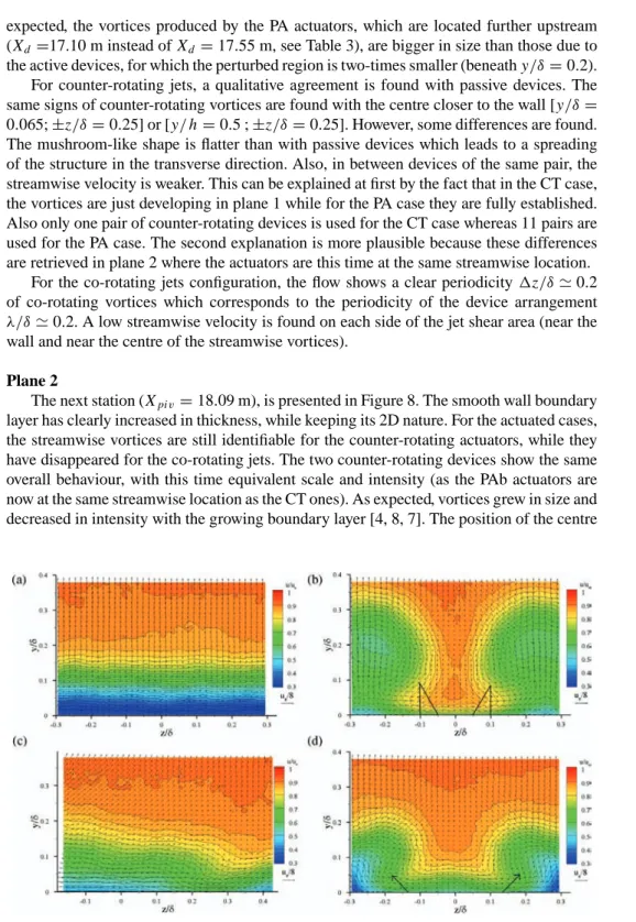
Plane 2

The next station (Xpiv=18.09 m), is presented in Figure 8. The smooth wall boundary

layer has clearly increased in thickness, while keeping its 2D nature. For the actuated cases, the streamwise vortices are still identifiable for the counter-rotating actuators, while they have disappeared for the co-rotating jets. The two counter-rotating devices show the same overall behaviour, with this time equivalent scale and intensity (as the PAb actuators are now at the same streamwise location as the CT ones). As expected, vortices grew in size and decreased in intensity with the growing boundary layer [4, 8, 7]. The position of the centre

Figure 8. Plane 2: WAC, PADb, CO and CTD. The black triangular in the PAD case represents the passive devices projected on the y-z plan. The Black arrows represent the jet direction from the active devices.

of vortices is approximately (y/δ=0.065;±z/δ=0.15] or [y/ h=0.79;±z/λ=0.30) for both counter rotating devices, which indicates that no significant lateral movement of the streamwise vortices is observed (±z/λ=0.3 for the first two PIV plane locations). On the contrary, the vortices have moved away from the wall in the same ratio as the growth of the TBL without actuation (y/δ =0.065 for the first two PIV plane locations). This indicates that the wall normal scaling for the mean vortex path is ratherδthanhcontrary to Logdberg et al. [7]. As at the previous station, the mushroom-like shape is flatter for active devices with a weaker streamwise velocity in the very near wall region. Also, in between devices of the same pair, the streamwise velocity is weaker for the jet VGs.

For co-rotating devices, a very different behaviour is found, even if the field of view is obviously too small for this case, the wake of the VGs has turned into a region of momentum downwash towards the wall, region which has moved to the right of the figure, due to self induction of the co-rotating vortical motion near the wall. Nevertheless, the BL momentum is improved in the whole region of observation.

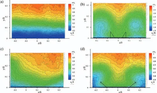
Plane 3

At the last streamwise stationXpiv=18.57 m (Figure 9), which is nearly the minimum

skin friction station, the smooth wall BL has again increased in thickness. The slight transverse asymmetry should be attributed to the PIV accuracy which was a bit less in this configuration, due to some difficulties to adjust the set-up. The field of view is obviously too small for the co-rotating jets. Although some significant momentum downwash is visible, it would be interesting to assess the flow on both sides of the field of view. For the counter-rotating passive devices, the results show an homogenisation, with a streamwise velocity in the range of 0.5 to 0.7 Ue, all down to the wall. The vortices trace, although fairly weak, is still detectable. The counter-rotating jets show still fairly coherent vortices. The data gives

Figure 9. Plane 3: WAC, PADb, CO and CTD. The black triangular in the PADb case represents the passive devices projected on the y-z plan. The Black arrows represents the jet direction from the active devices.

an evidence of alternations of low and high momentum regions near the wall, but with an increase everywhere, as compared to the smooth wall.

Summary

For an equivalent efficiency, around 200% of shear stress gain compared to the non-actuated case (see Godard and Stanislas [2]), the PIV results in the three planes of ob-servation evidence little differences between PA and CT and high differences between CT and CO devices. The evolution for the streamwise vortices produced by counter-rotating vortices are overall similar to the literature. The longitudinal evolution from co-rotating configuration is subject to too few studies to be compared, although Lin [4] reports it to be more efficient in 3D cross-flow configurations than in 2D configurations. In this study, the initial individual vortices are observed to merge into a large single vortical region which has the ability to globally increase the momentum near the wall.

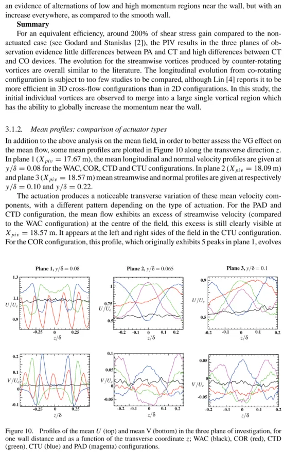
3.1.2. Mean profiles: comparison of actuator types

In addition to the above analysis on the mean field, in order to better assess the VG effect on the mean flow, some mean profiles are plotted in Figure 10 along the transverse directionz. In plane 1 (Xpiv=17.67 m), the mean longitudinal and normal velocity profiles are given at

y/δ=0.08 for the WAC, COR, CTD and CTU configurations. In plane 2 (Xpiv=18.09 m)

and plane 3 (Xpiv=18.57 m) mean streamwise and normal profiles are given at respectively

y/δ=0.10 andy/δ=0.22.

The actuation produces a noticeable transverse variation of these mean velocity com-ponents, with a different pattern depending on the type of actuation. For the PAD and CTD configuration, the mean flow exhibits an excess of streamwise velocity (compared to the WAC configuration) at the centre of the field, this excess is still clearly visible at Xpiv=18.57 m. It appears at the left and right sides of the field in the CTU configuration.

For the COR configuration, this profile, which originally exhibits 5 peaks in plane 1, evolves

0.25 -0.25 0.25 0 -0.1 0.1 0.1 0 -0.1 0 1 0 0 0 z/δ z/δ z/δ z/δ z/δ -0.25 z/δ Plane 2, y/δ=0.065 Plane 1, y/δ=0.08 Plane 3, y/δ=0.1 V/Ue V/Ue -0.1 -0.2 0.1 0.2 -0.2 0.2 0.2 -0.2 -0.1 0.1 0.2 -0.2 0.1 0.05 -0.05 0.2 0.1 -0.1 0.9 0.5 0.5 0.9 0.05 -0.05 V/Ue U/Ue U/Ue U/Ue 0.75 1.1 1.3 0 0 0

Figure 10. Profiles of the meanU(top) and mean V (bottom) in the three plane of investigation, for one wall distance and as a function of the transverse coordinatez; WAC (black), COR (red), CTD (green), CTU (blue) and PAD (magenta) configurations.

downstream such as a global increase of the streamwise velocity is noticeable in planes 2 and 3 with a maximum aroundz/δ=0.25. In all the actuated cases, a global acceleration of the flow is observed. It can also be noticed that a maximum of streamwise velocity corresponds to a negative minimum of the normal component and a minimum of streamwise velocity corresponds to a positive maximum ofV (except for the COR configuration in plane 3, where no extrema is clearly noticeable on the normal velocity profile). Actually, negative normal velocity corresponds to a transport of high-speed fluid from the free-stream. On the contrary, positive normal velocity corresponds to a transport of low-speed fluid outside the boundary layer. A clear difference in behaviour between co- and counter-rotating devices can be noticed. For the COR, in plane 1 and at the chosen altitude, a momentum deficit appears on average compared to the WAC case. This is due to the fact that the vortices are compactly staggered near the wall and leave little room between them for downwash. In planes 2 and 3, the individual vortices of plane 1 have merged together. The momentum benefit is clearly visible and the wake of the actuating device has moved transversely by self induction. For the different counter-rotating configurations, the lifetime of the individual vortices is much longer and the momentum transfer is in evident agreement with the sign and location of the different vortices. One solution to avoid the merging in the co-rotating case would be to increase the transverse spacing, but it has been shown by Godard and Stanislas [1, 2] that this reduces the overall efficiency of the device.

3.2. Turbulent kinetic energy

Besides the mean velocity, it is of interest to plot an indicator of the turbulence activity in the flow: the turbulent kinetic energy k. As the measurement were performed with stereo PIV, this quantity, which is half the trace of the Reynolds stress tensor is directly accessible. Figure 11 shows this quantity in the first measurement plane and for the different configurations tested. Without actuation (WAC) the turbulent activity is located, as expected, very near the wall aty <0.1δ. In all the actuated cases,kis enhanced significantly by the actuation and located mainly in the wake of the actuators. This indicates that the vortices

Figure 11. Turbulent kinetic energy – from top left to bottom right: WAC, CTD, CTU, COR, PAD, PAU configurations (plane 1).

Figure 12. Turbulent kinetic energy (plane 2).

are probably slightly fluctuating in position, due to their interaction with the oncoming turbulence. In plane 2 (Figure 12), the situation has evolved significantly. First, without actuation,k has increased significantly, and the peak has moved away from the wall (in agreement with the previous HWA measurements of Bernard et al. [31]). In the actuated cases, the level ofkis comparable to the WAC case and it seems that the turbulent activity has been gathered in some preferable areas of the flow. This is mainly the upwash region for the counter rotating configurations and the left part of the field, where turbulence has

been spread as compared to the WAC case, for the co-rotating configuration. In plane 3 (Figure 13), which is far downstream (in the region of minimum wall shear stress) the turbulence peak is still intense. In the WAC case, it is wider and further away from the wall, in agreement with previous hot wire measurements [31]. The counter-rotating actuators clearly redistributekat the top of the upwash regions. For the co-rotating case, the results are difficult to interpret.

As a conclusion, the actuators seem to generate turbulence in plane 1. This ‘apparent’ turbulence is probably due to the fluctuation in position of the vortices, as it becomes rapidly comparable in intensity to the natural one (planes 2 and 3). The actuation seems to redistribute spatially this turbulence. This is particularly evident for the counter-rotating actuators.

4. Spatial correlations

Spatial correlation is classically used to reveal the underlying organisation of turbulent flows. In the present case, in order to asses the organising ability of the streamwise vortices, we have computed the two points spatial correlation of the velocity fields. The two point spatial correlation co-efficients are defined as the temporal mean value of the following relation:

Rij(x, −→dx, t)=

ui(x, t). uj(x+ −→dx, t)

ui(x, t). ui(x, t) uj(x+ −dx, t).→ uj(x+ −→dx, t)

. (1)

The vectorxis a two-component vector in the plane (y, z), and it represents the coordinates of a fixed point,−dx→represents the coordinates of the moving point, andt is the time. In the present case, an ergodicity hypothesis is used: the average is not computed on time but as an ensemble average on the number of PIV maps which are supposed completely uncorrelated (this is true as the time separation between two maps is much larger than the time scale of the Taylor macro scales of the flow).

In all the results presented below, the direction normal to the wall is considered as the non-homogeneous direction. The transverse direction will sometimes be considered homogeneous. In this case, the correlation coefficients are averaged along thezdirection, and the fixed point is then defined by its single wall normal coordinatey.

4.1. Without actuation

First, the different spatial correlation coefficients in planes 2 and 3 in the configuration without actuation (referred to as WAC) were computed. In this particular case, the transverse directionzis considered as homogeneous. Figures 14 and 15 show these coefficients. The altitude of the fixed point isy/δ=0.065 for plane 2 and y/δ=0.010 for the plane 3. These altitudes correspond more or less to the centre of the vortices, when the actuators are in operation. As can be seen, the normal coefficientsR22andR33 are fairly localised, with an increase of the scales when going downstream. The wall normal velocity gradient is detectable in plane 2 onR22 as the correlation is computed here on the instantaneous velocities and not on the fluctuations. The cross correlation coefficientsR23andR32show a shape which has already been observed by Bernard et al. [31] and which is typical of vortices normal to the PIV plane. Again, the size of these vortices increases downstream.

Figure 14. Spatial correlation coefficients for the configuration without actuation (WAC); plane 2; fixed point aty/δ=0.065.

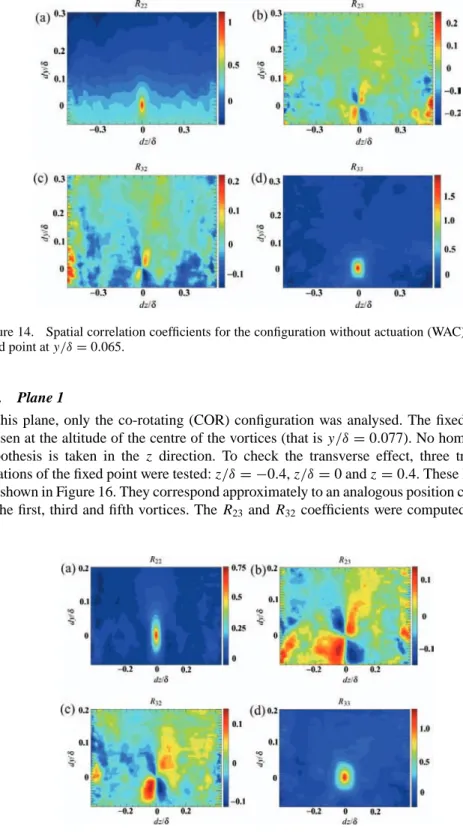
4.2. Plane 1

In this plane, only the co-rotating (COR) configuration was analysed. The fixed point is chosen at the altitude of the centre of the vortices (that isy/δ=0.077). No homogeneity hypothesis is taken in the z direction. To check the transverse effect, three transverse locations of the fixed point were tested:z/δ= −0.4,z/δ=0 andz=0.4. These locations are shown in Figure 16. They correspond approximately to an analogous position compared to the first, third and fifth vortices. TheR23 andR32 coefficients were computed, as they

Figure 15. Spatial correlation coefficients in for the configuration without actuation (WAC); plane 3; fixed point aty/δ=0.010.

Figure 16. Mean velocity field; plane 1; COR configuration; location of the three fixed points a, b and c.

indicate the links between the normal and transverse components of the velocity. The results are shown in the Figure 17. The two coefficients show a fairly different shape. Looking first atR23close to the fixed point, it shows a structure which looks like the right half of the same figure in the WAC case. This can be explained by the fact that the vortex is now located on average on the right side of the fixed point, while in the WAC case, streamwise vortices are randomly distributed. The size of the half butterfly shape is now scaled by the actuating vortices. This half butterfly is repeated periodically at each vortex location, indicating a strong transverse correlation between the vortices of the array. TheR32coefficient shows also a half butterfly shape near the fixed point, but this time it is the lower two lobes which are kept and which repeat themselves transversely. Curiously, the periodicity is less clear

Figure 17. R23 (top) andR32 (bottom) for the three fixed point (a), (b) and (c); plane 1; COR configuration.

at point b, but this should be attributed to a lack of convergence as only 200 samples are available to compute the correlation coefficients when no homogeneity hypothesis is used. In fact a slightly better convergence could be achieved by averaging the three maps of Figure 17.

4.3. Plane 2

In this plane, the fixed point altitude was chosen to correspond to the centre of the vortices generated by the counter-rotating jets configuration, that is y/δ=0.065. First, the R23 coefficient was computed in the CTD, CTU and PADb configurations. The transverse direction is again considered as non-homogeneous, and the fixed point is located atz/δ=0. Figure 18 shows the mean velocity field with the location of the fixed point, and the corresponding iso-contours of theR23coefficient in these three configurations. In the CTD and PADb configurations, at the fixed point, the mean dynamic of the flow indicates that high-speed fluid is directed towards the wall (i.e. high negative normal component of the velocity at this point), and in the CTU configuration the mean dynamic of the flow indicates that low-speed fluid is ejected from the wall towards the free-stream (i.e. high positive normal component of the velocity at this point). The butterfly shape of theR23 coefficient, observed in the WAC configuration (Figures 14 and 15) is clearly observable here again but with two important differences. First, in the present situation, counter-rotating streamwise vortices are existing on average on both sides of the fixed point, while in the WAC configuration single streamwise vortices of both signs are randomly distributed in the field. Secondly, the correlation pattern scales obviously here on the size of the actuating vortices which, by comparing Figures 18 and 14, appear about two-times larger than the natural streamwise structures of the TBL at this location. It must be recalled at this stage that these actuating configurations have been found optimum by the parametric study of Godard and Stanislas [1, 2]. One further point which should be noted is the fact that in the passive (PADb) configuration, the order of magnitude of the wall extrema is approximately two-times higher than in the CTD configuration. This is associated with a less noisy correlation

Figure 18. Mean velocity field (top) and iso-contours ofR23(bottom) in the CTD, CTU and PADb configurations; fixed point located aty/δ=0.065 andz/δ=0; plane 2.

Figure 19. Mean velocity field with the location of the two fixed points PF1 and PF2 and iso-contours ofR23andR32; COR configuration; plane 2.

as compared to the two other cases, indicating that the BL turbulence is less affecting the actuating flow in this passive device case at this location.

In a second step, theR23 coefficient was computed in the COR configuration for two fixed points: one aty/δ=0.065 andz/δ=0 as previously (PF1), and the second one at y/δ=0.065 cm andz/δ=0.25 (PF2). Figure 19 shows the mean velocity field with the two fixed points and the iso-contours of theR23andR32 coefficients for these two cases. The shape ofR23 looks at a first glance fairly different from the counter-rotating case. A close look leads to interpret it as a single half-butterfly pattern similar to the periodic one observed in plane 1 (Figure 17) but symmetric of it. This interpretation is coherent with the existence of a large and flat clockwise vortical motion on the left part of the field (in Figure 17 the vortex was on the right side of the fixed point). This large coherent area was already interpreted by Godard and Stanislas [2] as the merging of the individual vortices identified in plane 1. The correlation is much stronger at point PF2 which is at the right border of the actuated area than at point PF1 which is in the actuated area and at the altitude where the transverse velocity component changes sign. Anyway, as in plane 1, the actuated flow shows a strong transverse correlation. As far as theR32coefficient is concerned, in both the PF1 and PF2 cases, a fairly wide and significant positive peak is observed at the right of the fixed point. This can be explained by a downwash motion induced by the large vortical region located on the left of the field. The wide transverse correlation is more difficult to interpret.

Finally, the R23 and R32 coefficients were computed in the WAC, CTD, PADb and COR configurations, withzbeing considered as an homogeneous direction. The results are shown in the Figures 20 and 21. Apart for the co-rotating case, a strong analogy in shape is observable for both coefficient between the actuated and non-actuated cases. The size and strength vary significantly between the WAC and the actuated cases and also between the two types of actuation. The two correlation coefficients are fairly similar in size, shape and strength in the WAC case, whileR23shows a much stronger correlation thanR32for the two counter-rotating actuators. The actuating structures appear here three to four-times bigger than the natural streamwise vortices of the BL. The passive devices (PADb) induce a much

Figure 20. R23iso-contours; fixed point altitudey/δ=0.065,zhomogeneous; plane 2.

stronger correlation than the jets system (CTD). In the co-rotating configuration (COR), the two correlation coefficients are strong too but show a fairly different shape, which is coherent with the results of Figure 19. These results clearly indicate that the counter-rotating actuation induces a mechanism which is similar to the natural one, but stronger and with larger structures while the co-rotating actuation changes significantly the boundary layer flow structure.

Figure 22. R23iso-contours; fixed point altitudey/δ=0.010,zhomogeneous; plane 3.

4.4. Plane 3

As previously, the fixed point altitude corresponds to the centre of the vortices generated by the counter-rotating jets configuration. This is nowy/δ=0.065. In this plane, due to the limited number of samples, correlations computed without homogeneity hypothesis are very noisy. The transverse direction was thus considered homogeneous to computeR23and R32. These coefficients are shown in the Figures 22 and 23, for the WAC, CTD, PADb and

COR configurations. They can be compared to the same data in plane 2 shown in Figures 20 and 21. Obviously, even with the homogeneity hypothesis, a larger number of samples would be of worth. As far as the shape of the correlations are concerned, the same conclusions as in plane 2 can be drawn for the counter-rotating actuators. The main difference is in the comparison of the size and strength between the actuated and non-actuated flow. They are now fairly comparable for the WAC and the CTD. The PADb being slightly stronger near the wall. Two explanations can be given to these results: either the actuating vortices have disappeared and the natural flow structures have reorganised themselves or the actuating vortices which, by comparing Figures 22 and 23 with Figures 20 and 21, appear to stay more or less constant in size, become in plane 3 of the same size as the local natural structures without actuation. Looking at the instantaneous velocity maps, the reality is somewhere in between: the actuating vortices are still present but they are mixed in the turbulent structures coming from upstream and more difficult to individualise.

5. Vortex detection and characterisation method 5.1. Detection function

Finding a reliable mathematical criterion to define a vortex is a subject which has been thoroughly addressed and which will not be discussed in detail here. Different detection functions are proposed, which are reviewed for example by Jeong and Hussain [34]. They all originate from the velocity gradient tensor∇ uwhich shows three main invariants:P =ui,i,

Q=1

2ui,juj,iandR=Det(ui,j). The corresponding detection functions are:

r

2(ui,j−uj,i)|

2_{; its value is related to the intensity of vortices.}

r

2_{, which indicates a vortex when taking} positive values.

r

r

In the following,Qwill be used as detection function.

All the detection functions previously defined need the use of a derivation filter. Some derivation schemes provide too noisy data, whereas other schemes have a strong smoothing effect. After testing various filters, we found that the 2nd order least square filter, which is defined as: ∂u ∂x(xi)= 1 17[u(xi+x)−u(xi−x)]+ 4 17[u(xi+4x)−u(xi−4x)], which is the best compromise, and will be used in the following.

5.2. Indicative function

Having defined a detection function, a second step is to construct from it an indicative func-tion. Usually, this is done by thresholding the detection funcfunc-tion. This indicative function is then binary with a value of 1 at the points where the object is detected.

The difficulty here is to choose the right threshold for the detection function. We have first scaled the detection function as an 8 bits image, i.e. with values from 0 to 255. This

Figure 24. Vortex detection in the CTD configuration for fields number 20, 40, 100 and 150; plane 2; (a) detection function scaled between 0 and its maximum; (b) detection function scaled between 0 andQ+_mean+Q+_mean; (c) indicative function; (d) indicative function after filtering with a disc of radius 1.

was necessary to use available mathematical morphology tools. We did it in such a way that all the negative values ofQare 0 (black), and the maximum positive value ofQis 255 (white). Thus, for all the positive values ofQthe grey level goes from black to white. This is illustrated in Figure 24(a) for the instantaneous field number 20, 40, 100 and 150 in the CTD configuration in plane 2. As can be seen, the images obtained are quite dark. This is due to the fact that, most often, some tiny bright peaks appear on the border of the field. We thus decided to scale the detection function differently:

r

r

The result of this scaling is shown in Figure 24(b). As can be seen, the vortical elements are clearly evidence by this scaling.

The next step is to select the value of the threshold. Looking at a sample of fields larger than the one shown in Figure 24, it appears that a threshold Th∼8% ofQ+_mean+Q+_mean (that is a grey level of 20 in the present case) is a good compromise between the amount of noise and the relevant vortical structures detected. Figure 24(c) shows the indicative function obtained from the detection functions of Figure 24(b) with this value of the threshold.

5.3. Structure extraction

The last step is the extraction of the information we want (the vortices) based on the indicative function. The binary image representation of this indicative function usually

Figure 25. Example of the dilatation and erosion operations.

needs to be filtered, which may be performed using mathematical morphological functions. More information about mathematical morphology may be found in Serra [35].

As evidenced by Figure 24(c), after thresholding, noise exists in the binary images (the indicative functions) such as small structures, small holes inside structure, etc.

In order to filter this noise, morphological filters were applied. The procedure used was the following: an opening (erosion + dilatation) operator followed by a closing (dilatation + erosion) operator. The opening operation smooths the contours of the structures, cuts the narrow isthmuses and suppresses the small islands and the sharp capes. On the other hand, the closing operation blocks up the narrow channels, the small lakes and the long thin gulfs. These two operations are the combination of two fundamentals operators: erosion and dilatation. Let us consider a digital image in which there is a structureX(set of pixels equals to 1), and also consider a structuring elementB. The principle of the erosion and dilation operations are briefly illustrated with an example ofX andB in Figure 25. The dilatation ofXbyBis the union of the black and shaded red pixels, and the eroded ofX byBis the remaining black pixels.

In the present case, different structuring element were tried. The one which seemed the most convenient was a disc of radius 1, i.e. a structuring element of the following form:

0 1 0 1 1 1 0 1 0 .

Figure 24(d) shows the filtered image, obtained from the indicative functions of Figure 24(c), using the above described procedure. In order to distinguish between the positive and negative vortices, the binary images obtained were finally multiplied by the vorticity sign.

Figure 26. WAC configuration, plane 1; (a) loci of the vortex centres; (b) and (c) histograms of the number of vortex detected as a function of, respectively,zandy.

5.4. Structure characterisation

The structures which remain after all the operations previously described are labelled in order to perform statistical operations on them. It is then possible to compute the average number of structures (positive and negative), the average perimeter, surface, radius, altitude, etc. The histograms of the number of structures, structures altitude and transverse positions can also be plotted. The results are presented in the next section.

5.5. Results

5.5.1. Plane 1

In order to show the influence of jets actuation on the vortices organisation inside the boundary layer, a vortex detection was first performed for the WAC configuration. Figure 26(a) shows the loci of the vortices centres obtained by analysing the 200 velocity fields available. The red stars correspond to positive (clockwise) vortices, and the blue stars to negative (counter-clockwise) vortices. Figures 26(b) and 26(c) show the histograms of the number of vortices as a function of, respectively, the transverse and normal coordinates. The vortices are homogeneously distributed in the transverse direction, and preferably near the wall where the concentration increases strongly. Approximately four vortices of each sign were detected on the instantaneous fields, showing that the two kinds are equally probable. The average characteristics of these vortices are summarised in Table 4. These are the radius R and the intensity . The intensity is here a vorticity. The maximum (or minimum) value of the streamwise vorticity component is retained for each structure. This value is averaged over all the detected structures. The small differences between the two types of structures should be attributed to a lack of convergence. At this station, the friction velocity isuτ=0.365, which givesR+ =Ruτ/µ∼73 and += u2τ/µ∼2.10−

4_. The left part of Figure 27 shows the mean velocity maps, while the right part shows the loci of the centres of the vortices detected respectively in the COR and CTD configuration. We first notice that the pattern of the vortices locations is analogous to the pattern we could anticipate from the mean velocity field (left part of Figure 27), which means that the vortices generated by the jets actuation devices (which are located just upstream this plane 1) are relatively steady. For the COR configuration, around 77% of the vortices detected are positive, and the negative vortices are located between the positive ones near the wall as shown in Figure 27. Figure 28(a) shows the histogram of the number of vortices detected as a function of the transverse coordinate. This histogram exhibits five predominant transverse locations for the positive vortex, and it also confirms that negative vortices are

Figure 27. Mean velocity field and loci of the centres of the positive (red) and negative (blue) vortices; (top) COR, (bottom) CTD; plane 1.

dominant between these five locations. Figure 28(b) represents the histogram of the number of vortices detected as a function of the normal coordinate. The positive vortex are dominant aroundy/δ=0.05, while the negative ones show a two peaks histogram: very near the wall (y/δ∼0) and just above the positive vortices (y/δ∼0.13). The average characteristics of these vortices are summarised in the Table 4. The positive vortices have a radius almost two-times larger than the negatives ones, and their intensity is 67% higher. Both vortices are stronger than the natural ones (Table 4). The positive ones are 56% larger and the negative

Figure 28. Histograms of the number of vortices detected (red: positive, blue: negative); (a) with respect toz; (b) with respect toyin the COR configuration; (c) with respect toz; (d) with respect to

Table 4. Average characteristics of the vortices detected in plane 1.

Config Features R (mm) (rad/s)

WAC Positive vortices 2.97 1.72

Negative vortices 3.09 −1.59

COR Positive vortices 4.66 3.83

Negative vortices 2.39 −2.56

CTD Positive vortices 4.14 2.44

Negative vortices 4.16 −2.73

ones 25% smaller. The comparison of the top two images of Figure 27, together with the value of the mean radius of the positive vortices in this case (R∼4.7 mm) indicates that the average velocity map of Figure 27 is in fact the result of the unsteady motion of vortices which are much smaller than what this mean map indicates. The negative vortices put in evidence by the detection procedure in the right map of Figures 27 are not at all visible in the averaged velocity map. They are slightly smaller than the vortices detected in the WAC case (Table 4). They can be either secondary vortices generated in the interaction of the actuators jets with the mean flow or negative streamwise structures from the boundary layer segregated and stretched by the actuating flow. The positive ones would then be ingested by the main actuating vortices, which would explain partly their unsteadiness so near from the actuators.

For the CTD configuration (Figure 27 bottom), in addition to the two locations we could anticipate from the mean velocity field (two counter-rotating vortices), we also notice a high density of negative vortices at the left of the positive vortex, and a high density of positive vortices at the right of the negative vortex. The spatial spreading of these secondary vortices is significantly higher than that of the main ones. The histogram of Figure 28(c) confirms the existence of these two domains of vortex population close to the left and right edges of the image and aroundz/δ= −0.24 andz/δ=0.24. The altitude of both the negative vortices is aroundy/δ=0.05 and a bit further for the positive vorticesy/δ=0.06 as shown in the Figure 28(d). As much positive as negative vortices were detected (three of each kind on average). Table 4 summarises their mean characteristics. We can notice the similarity between the positive and negative vortices in terms of size and intensity, which constitutes the main difference compared to the COR configuration. Here, both vortices are stronger than in the WAC case.

5.5.2. Plane 2

Figure 29(a) shows the loci of the centres of the detected vortices for the WAC configuration, while Figure 30 gives the same data for the COR, CTD, CTU and PADb configurations. Figures 29(b), 29(c), 31 and 32 give the corresponding histograms.

In the WAC case, the distribution is still equiprobable and homogeneous inz, but the wall region, where the population is high, has extended significantly away from the wall. This is clearly seen both in Figures 29(b) and 29(c). Table 5 gives the mean characteristics. The radius has increased by about 20% and the intensity has diminished by the same percentage as compared to plane 1. A higher concentration of positive vortices is observed in the COR configuration compared to the WAC case. These positive vortices are especially dominant on the left part of the field (z/δ <0.16). The histograms of Figure 31(a)–32(a) confirm the dominance of these positive vortices in the region where the large scale motion has been

Figure 29. (a) Loci of the centres of vortices detected in the WAC configuration; (b) histogram with respect toz; (c) histogram with respect toy; plane 2.

Figure 30. Loci of the centres of vortices detected (red: positive, blue: negative); (a) COR, (b) CTD, (c) CTU, (d) PADb; plane 2.