Uncertainty Quantification of Wall-Modeled Large Eddy Simulation (WMLES) Model in OpenFOAM

Washington University in St. Louis

Washington University Open Scholarship

Engineering and Applied Science Theses &

Dissertations McKelvey School of Engineering

Spring 5-15-2017

Uncertainty Quantification of Wall-Modeled Large

Eddy Simulation (WMLES) Model in

OpenFOAM

Zuoxian Hou

Washington University in St. Louis

Follow this and additional works at:https://openscholarship.wustl.edu/eng_etds

Part of theEngineering Commons

This Thesis is brought to you for free and open access by the McKelvey School of Engineering at Washington University Open Scholarship. It has been accepted for inclusion in Engineering and Applied Science Theses & Dissertations by an authorized administrator of Washington University Open Scholarship. For more information, please [email protected].

Recommended Citation

Hou, Zuoxian, "Uncertainty Quantification of Wall-Modeled Large Eddy Simulation (WMLES) Model in OpenFOAM" (2017).

Engineering and Applied Science Theses & Dissertations. 253.

WASHINGTON UNIVERSITY IN ST. LOUIS School of Engineering and Applied Science

Department of Mechanical Engineering and Material Science

Thesis Examination Committee: Ramesh Agarwal, Chair

Dave Peters Swami Karunamoorthy

Uncertainty Quantification of Wall-Modeled Large Eddy Simulation (WMLES) Model in OpenFOAM

by Zuoxian Hou

A dissertation presented to the School of Engineering and Applied Science of Washington University in St. Louis in partial fulfillment of the

requirements for the degree of Master of Science

May 2017 St. Louis, Missouri

ii

Table of Contents

Table of Contents ... ii List of Figures ... iv List of Tables ... vi Acknowledgments... vii ABSTRACT OF THESIS ... ix Chapter 1: Introduction ... 1 1.1 Motivation ... 1

1.2 Brief Review of Literature ... 1

1.2.1 Large Eddy Simulation (LES) ... 1

1.2.2 Uncertainty Quantification (UQ) ... 2

1.3 UQ Software ... 3

1.4 Flow Simulation Software ... 3

Chapter 2: Review of Uncertainty Quantification (UQ) and Large Eddy Simulation (LES) ... 4

2.1 Introduction to Uncertainty Quantification (UQ) ... 4

2.2 Large Eddy Simulation (LES) ... 7

2.2.1 Smagorinsky Model ... 9

2.2.2 Wall-Modeled Large Eddy Simulation (WMLES) ... 10

Chapter 3: Validation of LES Result ... 12

3.1 Comparison of Velocity Profiles at Reτ = 395 ... 12

3.2 Comparison of Velocity Profiles at Reτ = 550 ... 13

3.3 Comparison of Velocity Profiles at Reτ = 2000 ... 14

3.4 Comparison of Velocity Profiles at Reτ = 5200 ... 15

3.5 Conclusions ... 16

Chapter 4: Mesh and Boundary Conditions ... 17

4.1 Mesh and Boundary Conditions at Reτ = 395 ... 17

4.2 Mesh and Boundary Conditions at Reτ = 550 ... 18

4.3 Mesh and Boundary Conditions at Reτ = 2000 ... 18

iii

Chapter 5: UQ of Skin Friction Coefficient with Smagorinsky and WMLES models ... 21

5.1 Sobol Indices for Skin Friction Coefficient ... 21

5.1.1 Sobol Indices for Reτ = 550 ... 21

5.1.2 Sobol Indices for Reτ = 2000 ... 22

5.1.3 Sobol Indices for Reτ = 5200 ... 22

5.2 Change in Skin Friction Coefficient with Change in Coefficients of Smagorinsky and WMLES model ... 23

5.2.1 Change in Skin Friction Coefficient in Smagorinsky Model ... 23

5.2.2 Change in Skin Friction Coefficient in WMLES Model ... 24

5.3 Conclusions ... 25

Chapter 6: UQ of Mean Velocity Profiles from Smagorinsky and WMLES Model ... 27

6.1 UQ of Velocity Profile when Reτ = 550 ... 27

6.1.1 UQ of Velocity Profile from Smagorinsky Model ... 27

6.1.2 UQ of Velocity Profiles for WMLES Model ... 29

6.2 UQ of Velocity Profile when Reτ = 2000 ... 31

6.2.1 UQ of Velocity Profile from Smagorinsky Model ... 31

6.2.2 UQ of Velocity Profile for WMLES Model ... 33

6.3 UQ of Velocity Profile when Reτ = 5200 ... 35

6.3.1 UQ of Velocity Profile from Smagorinsky Model ... 35

6.3.2 UQ of Velocity Profile for WMLES Model ... 37

Chapter 7: Conclusions ... 40

Chapter 8: Future Work ... 41

References ... 42

iv

List of Figures

Figure 3.1 Comparison of velocity profiles for fully developed turbulent flow in a channel using

the LES with original Smagorinsky model, the modified Smagorinsky model and DNS at Reτ =

395………..………12

Figure 3.2 Comparison of velocity profiles for fully developed turbulent flow in a channel using the LES with the Smagorinsky model, the WMLES model and DNS at Reτ = 5200…...…13

Figure 3.3 Comparison of velocity profiles for fully developed turbulent flow in a channel using the LES with the Smagorinsky model, the WMLES model and DNS at Reτ = 5200………14

Figure 3.4 Comparison of velocity profiles for fully developed turbulent flow in a channel using the LES with the Smagorinsky model, the WMLES model and DNS at Reτ = 5200……...15

Figure 4.1 Mesh and boundary conditions at Reτ = 395 ………..……..………..17

Figure 4.2 Mesh and boundary conditions at Reτ = 550 ………...……..18

Figure 4.3 Mesh and boundary conditions at Reτ = 2000 ………...………19

Figure 4.4 Mesh and boundary conditions at Reτ = 5200 ………...………20

Figure 6.1 Sobol indices along the y direction for Smagorinsky model at Reτ = 550….………..28 Figure 6.2 Comparison of velocity profiles obtained by increasing 𝐶_𝑘 by 20% and 10% for Smagorinsky model with DNS data at Reτ = 550.……….………...….29 Figure 6.3 Sobol indices along the y direction for WMLES model at Reτ = 550………..30

Figure 6.4 Comparison of velocity profile obtained by decreasing 𝜿 by 20% and 10% for WMLES

model with DNS data at Reτ = 550………...31

Figure 6.5 Sobol indices along the y direction for Smagorinsky model at Reτ = 2000………….32

Figure 6.6 Comparison of velocity profiles obtained by increasing 𝐶_𝑘 by 20% and 10% for

Smagorinsky model with DNS data at Reτ = 2000………...…….….33

Figure 6.7 Sobol indices along the y direction for WMLES model at Reτ = 2000.………..34

Figure 6.8 Comparison of velocity profiles obtained by increasing 𝜿 by 20% and 10% for WMLES

model with DNS data at Reτ = 2000………...35

v

Figure 6.10 Comparison of velocity profiles obtained by increasing 𝑪_𝒌 by 20% and 10% for

Smagorinsky model with DNS data at Reτ = 5200……….……...37

Figure 6.11 Sobol indices along the y direction for WMLES model at Reτ = 5200………..38

Figure 6.12 Comparison of velocity profiles obtained by decreasing 𝑪_𝜺by 20% and 10% for

vi

List of Tables

Table 2.1 Density and Weight Functions of Commonly Used Uni variate Optimal Basis

Functions………..5 Table 2.2 Epistemic Intervals of Closure Coefficients for Smagorinsky model ……….11 Table 2.3 Epistemic Intervals of Closure Coefficients for WMLES model ……….12

Table 5.1 Sobol indices for the skin friction coefficient from OpenFOAM when Reτ =550 …….21

Table 5.2 Sobol indices for the skin friction coefficient from OpenFOAM when Reτ =2000 …..22

Table 5.3 Sobol indices for the skin friction coefficient from OpenFOAM when Reτ =5200 …...23

Table 5.4 Sobol indices at various Reτ for Smagorinsky model by decreasing the coefficients by

10% ………...23

Table 5.5 Sobol indices at various Reτ for Smagorinsky model by increasing the coefficients by

10% ………...23 Table 5.6 Sobol indices at various Reτ for WMLES model by decreasing the coefficients by

10% ………...………24 Table 5.7 Sobol indices at various Reτ for WMLES model by increasing the coefficients by

10% ………...………24 Table 5.8 Sobol indices of a combination of two model coefficients for the skin friction coefficient from OpenFOAM for Smagorinsky model ……….………...25 Table 5.9 Sobol indices of a combination of two model coefficients for the skin friction coefficient from OpenFOAM for WMLES model ………..……….25

vii

Acknowledgments

I would like to thank to my parents, Yuhui Hou and Huan Wang, who taught me to be curious to everything and spirit of persistence in achieving the goal. I am grateful for their help in all aspects.

Many thanks to my research advisor, Professor Ramesh K Agarwal for providing me enormous help and guidance to improve my research skills. I would not have succeeded without his help. Thanks to Prof. Peters and Prof. Karunamoorthy for agreeing to serve on the thesis committee. I would like to thank Xu Han for providing enormous technical support in using the OpenFOAM and giving me confidence when I was disappointed. I would also like to thank Tim Wray and Issac Witte for teaching me how to use DAKOTA.

Finally, I want to thank to all my colleagues in the CFD lab. I had a meaningful and very pleasant time with all of them.

Zuoxian Hou

Washington University in St. Louis May 2017

viii

ix

ABSTRACT OF THESIS

Uncertainty Quantification of Wall-Modeled Large Eddy Simulation (WMLES) Model in OpenFOAM

by Zuoxian Hou

Master of Science in Mechanical Engineering Washington University in St. Louis, 2017 Research Advisor: Professor Ramesh K. Agarwal

In this thesis, a non-intrusive uncertainty quantification (UQ) method is used to improve the accuracy of a wall-modeled large eddy simulation (WMLES) model. Detailed UQ studies focusing on the closure coefficients of two LES models are performed. A non-intrusive polynomial chaos model is used to evaluate output sensitivities and uncertainties in the entire flow domain. The proposed UQ method allows for the investigation of specific flow features and phenomena within the domain. The results of the UQ analyses are then used to identify which turbulence model closure coefficients most influence the flow features of interest. Sobol indices of closure coefficients (𝐶_𝑘, 𝐶_𝜀 in Smagorinsky model and 𝐶_𝑘, 𝐶_𝜀, 𝜅, 𝐴+ in WMLES model) are obtained. Based on the magnitudes of Sobol indices, refinements are then made to the closure coefficients of interest to improve the accuracy of the turbulence models. OpenFOAM is used as the flow solver and the UQ analyses are conducted with DAKOTA. The UQ method is applied to the channel flow at different Reynolds numbers. The refined LES turbulence models with modified closure coefficients show improvement in the prediction of the skin-friction coefficient in the channel flow.

1

Chapter 1: Introduction

1.1 Motivation

Interest in uncertainty quantification (UQ) in computational fluid dynamics (CFD) has grown in recent years. UQ has been successfully applied to design, optimization, and modeling problems, and is becoming a standard tool for verification and validation of numerical solutions. The development of non-intrusive UQ methods has reduced the computational expense of UQ and has allowed uncertainty propagation through complex models without alteration to the underlying model.

In the present work, the sensitivities of the closure coefficients of the LES Smagorinsky model, and the wall-modeled large eddy simulation (WMLES) model are investigated. Flow calculations are performed with OpenFOAM. Turbulent channel flow at various Reynolds number is considered.

Non-intrusive polynomial chaos is used to propagate the uncertainty in the closure coefficients. DAKOTA is used to calculate the Sobol Indices which quantify the sensitivity of each coefficient to some physical quantity of interest. The main quantity of interest in channel flow is the coefficient of skin friction. Details of the two LES models, the flow solver, and the test case are given in the following sections. Results and discussions of the UQ analyses are presented. Closure coefficients of interest are identified.

1.2 Brief Review of Literature

1.2.1 Large Eddy Simulation (LES)

Most naturally occurring flows in real world are turbulent. Their simulation using the computational fluid dynamics (CFD) requires accurately modeling of turbulence. Unfortunately,

2

the computation of turbulence flows from first principles by Direct Numerical Simulation (DNS) of Navier-Stokes equations is currently not feasible at high Reynolds numbers because of the requirements of computational power, which is unlikely to be available in the foreseeable future. Therefore, turbulent flows are generally modeled employing the Reynolds-Averaged Navier- Stokes (RANS) equations or Large-Eddy-Simulation (LES). Both approaches require a turbulence model. In this thesis, the focus is on LES.

In LES, the large-scale motions in turbulent flow are solved by modified form of Navier-Stokes equations but the small scale eddies (sub-grid scale (SGS) eddies) require modeling. The most

well-known model for modeling the SGS eddies is the Smagorinsky model [1]. LES substantially

reduces the computational intensity compared to DNS and is more accurate than the RANS approach wherein the entire turbulence flow field is modeled using a turbulence model.

1.2.2 Uncertainty Quantification (UQ)

There are always differences between the computed results and the real world experimental data. Errors in the simulation results occur due to the approximations in modeling as well as due to uncertainty in numerical solution process. It is important to know which parameters in the physical and numerical model contribute most to the uncertainty. The uncertainties can be classified into two categories [2]:

a. Aleatoric uncertainty or “irreducible” uncertainty b. Epistemic uncertainty or “reducible” uncertainty

Aleatoric uncertainty is endogenous to the formulation; it represents the “known unknowns”. Epistemic uncertainty arises from lack of knowledge; this type of uncertainty is the focus of this thesis.

3

In CFD, the flow simulations are very sensitive to physical model and numerical parameters, such as the computational mesh, numerical algorithm turbulence model etc. In the AIAA CFD drag prediction workshops [3-7], it has been shown that the numerical parameters such as the quality of mesh, the order of the numerical scheme and turbulence model significantly influence the results. The focus of this thesis is on uncertainty quantification of different coefficients in the LES models and based on UQ analysis, these coefficients are modified to improve the prediction capability of these models.

1.3 UQ Software

The DAKOTA toolbox is used for UQ, it provides an adaptable and extensible interface between the simulation codes and an iterative framework consisting of several examination techniques. DAKOTA contains calculation methods for advancement with inclination and nongradient-based strategies; uncertainty quantification with testing, dependability, stochastic extension, and epistemic techniques; parameter estimation with nonlinear slightest squares techniques; and affectability/fluctuation examination with plan of analyses and parameter contemplate techniques.

1.4 Flow Simulation Software

OpenFOAM is a free, open source software released and developed primarily by OpenCFD Ltd. since 2004. It has a broad popularity base across the world. OpenFOAM has an extensive range of features to solve complex fluid flow problems involving chemical reactions, turbulence and heat transfer, as well as for solution of acoustics, solid mechanics and electromagnetics problems.

In the OpenFOAM, a solver called pimpleFoam is used in this thesis. It is applied to LES of incompressible turbulent flow in a channel at various Reynolds numbers.

4

Chapter 2: Review of Uncertainty

Quantification (UQ) and Large Eddy

Simulation (LES)

2.1 Introduction to Uncertainty Quantification (UQ)

In this review of UQ, the Quadrature-Based Non-Intrusive Polynomial Chaos (NIPC) theory is utilized. In the context of UQ, NIPC can transform an irregular random variable into separable

stochastic and deterministic parts as shown in Eq. (1), where α* could be any stochastic variable

of interest, for example, pressure or skin friction coefficient, lift or drag coefficient, or any other time-averaged value in a turbulent fluid flow problem.

𝛼∗_{(𝑡, 𝑥⃑, 𝜉⃑) ≈ ∑ 𝛼}

𝑗(𝑡, 𝑥⃑)Ψ𝑗(𝜉⃑) 𝑃

𝑗=0

(1)

In Eq. (1), Ψ_𝑗(𝜉⃑) is the stochastic basis function with respect to the mode of order j.α* is an element of the free deterministic variable vector (𝑡, 𝑥⃑)and the n-dimensional random variable vector 𝜉⃗ = (𝜉1, … , 𝜉𝑛); both aleatory and epistemic uncertain factors are incorporated into this condition. In this formulation, the polynomial chaos expansion (PCE) method is used since Eq. (1) ought to have boundless number of terms; however a discrete summation is assumed. To achieve an expansion of order p, the aggregate number of cases (Nt) is given by the Eq. (2):

𝑁𝑡 = 𝑃 + 1 = 𝑛𝑝

(𝑛 + 𝑝)!

𝑛! 𝑝! (2)

As shown in Eq. (2) Nt is a function of number of random dimensions (n) and the order of PCE

(p). When the input uncertainty is Gaussian, the basis function can be a multi-dimensional Hermite

Polynomial to develop the n-dimensional stochastic space, which was initially proposed by Wiener

5

arrangement of polynomials was utilized by Xiu and Karniadakis [9] as an Askey scheme to develop the Wiener-Askey Generalized Polynomial Chaos. The weight and density functions for few of the most widely used polynomials are shown in Table 2.1. As described in the review by Huyse et al. [10], the Hermite, Legendre and Laguerre polynomials are three most widely used basis functions.

Table 2.1 Density and Weight Functions of Commonly Used Univariate Optimal Basis Functions.

Input Distribution

Density

Function Polynomial Name

Weight Function Support Range (R) Normal 1 √2𝜋𝑒 −𝜉2 2 Hermite, 𝐻_𝑛(𝜉) _𝑒−𝜉₂2 [−∞, ∞] Uniform 1 2 Legendre, 𝐿𝑒𝑛(𝜉) 1 [−1,1] Exponential e−ξ Laguerre, 𝐿𝑎_𝑛(𝜉) e−ξ [0, ∞]

For an input uncertainty variable, there are three types of distribution called the Gaussian (typical), bounded (uniform) and semi-bounded (exponential). The ideal basis functions are the result of the weight functions multiplied by the standard probability density functions (PDF) of a known input uncertainty variable. The standard PDF must achieve the basic condition that the integration of the PDF over the whole range reaches a finite value. A direct consequence of this requirement is the multiplication between the density function and weight function which appear in Table 2.1. When there are more than one uncertainty variables, the multivariate basis functions can be obtained from orthogonal polynomials, as described in Eldred et al. [11]. For example, a multivariate Hermite polynomial can be obtained as

𝐻𝑛(𝜉𝑖1, … , 𝜉𝑖𝑛) = 𝐻𝑛(𝜉⃗) = 𝑒 1 2𝜉⃗⃗𝑇𝜉⃗⃗(−1)𝑛 𝜕 𝑛 𝜕𝜉_𝑖1, … , 𝜉_𝑖𝑛𝑒 −1_2𝜉⃗⃗𝑇_𝜉⃗⃗ (3)

6

Eq. (3) can also be obtained from one-dimensional Hermite Polynomials 𝜓_𝑚 𝑖

𝑗(𝜉_𝑖) by using the

multi-index m in another form as shown in Eq. (4):

𝐻𝑛(𝜉𝑖1, … , 𝜉𝑖𝑛) = Ψ𝑗(𝜉⃗) = ∏ 𝜓_𝑚 𝑖 𝑗( 𝑛 𝑖=1 𝜉𝑖) (4)

The fundamental data of the polynomial chaos strategy is to decide the coefficients in Eq. (1). At that point, the significance of how the information impacts the result can be ascertained by utilizing the p basis functions and these coefficients.

For example, Hosder et al. [12] have demonstrated that the mean value of a stochastic function is given by

𝜇_𝛼∗ = 𝛼⃑∗(𝑡, 𝑥⃑) = 𝐸_𝑃𝐶(𝛼∗(𝑡, 𝑥⃑, 𝜉⃑)) = ∫ 𝛼∗(𝑡, 𝑥⃑, 𝜉⃑)𝑝(𝜉⃑)𝑑𝜉⃑ = 𝛼₀(𝑡, 𝑥⃑)

𝑅

(5) Eq. (5) gives the expected or mean value of the output 𝛼∗(𝑡, 𝑥⃑, 𝜉⃑), it is simply the zeroth coefficient of the polynomial chaos expansion. Hosder et al. [12] show that there is an expression for changing the range of the output:

𝜇_𝛼2∗ = ∫ (𝛼∗(𝑡, 𝑥⃑, 𝜉⃑) − 𝛼₀∗(𝑡, 𝑥⃑)) 2 𝑝(𝜉⃑)𝑑𝜉⃑ 𝑅 = ∑[𝛼_𝑗2〈Ψ_𝑗2_〉] 𝑃 𝑗=1 (6) Equations (5) and (6) employ the fact that 〈Ψ𝑖Ψ𝑗〉 = 〈Ψ𝑗〉𝛿𝑖𝑗 and 〈Ψ𝑗〉 = 0 for j > 0, where 𝛿𝑖𝑗 is the Kronecker delta function. The dot product of Ψ_𝑖(𝜉⃑) and Ψ_𝑗(𝜉⃑) over the range R is defined as:

〈Ψ_𝑖(𝜉⃑)Ψ_𝑗(𝜉⃑)〉 = ∫ Ψ_𝑖(𝜉⃑)Ψ_𝑗(𝜉⃑)𝑝(𝜉⃑)𝑑𝜉⃑ 𝑅

(7) where 𝑝(𝜉⃑) is the probability density function.

In the event that the probability distribution of every stochastic variable is distinctive, the ideal multivariate basis functions can be obtained from the product of univariate quadrature polynomials utilizing the ideal univariate polynomial in each stochastic dimension. In this strategy, it is required

7

that the uncertainties utilized as input are independent typical stochastic factors. More insights about the polynomial chaos expansion can be found in the papers of Walters and Huyse [13], Najm [14], and Hosder and Walters [12]. Typically, two types of polynomial chaos, intrusive and non-intrusive are utilized for the uncertainty quantification in computational reproduction. Although straightforward in theory, an intrusive formulation for complex problems can be somewhat difficult and costly, and requires more resources to accomplish.

To overcome the disadvantages of the intrusive approach, non-intrusive polynomial chaos (NIPC) formulations is chosen for uncertainty quantification in this study.

2.2 Large Eddy Simulation (LES)

Large eddy simulation (LES) is a well-known model for simulating turbulent flows. A theory developed by Kolmogorov in 1941 showed that the large eddies in a turbulent flow are dependent on the geometry while the smaller eddies are universal. This concept was used in the formulation of LES model from the Navier-Stokes euqations.

In LES, the small-scale eddies near the wall of a turbulent boundary layer for example are modeled while the large scale eddies away from the wall are calculated directly by the Navier-Stokes equations. To accomplish this, filtering is performed. Filtering is defined as the convolution of a function u with a filtering kernel G:

𝑢̅𝑖(𝑥⃑) = ∫ 𝐺 (𝑥⃑ − 𝜉⃑)𝑢(𝜉⃑)d𝜉⃑ (8)

It results in

8

where 𝑢̅_𝑖 is the resolvable large scale part and 𝑢_𝑖′is the subgrid-scale part of variable u. However, most practical implementations of LES utilize the computational grid as the filter (the box filter) and do not employ explicit filtering.

The filtered equations can be obtained from the incompressible Navier-Stokes equations given below: 𝜕𝑢𝑖 𝜕𝑡 + 𝑢𝑗 𝜕𝑢𝑖 𝜕𝑥_𝑗 = − 1 𝜌 𝜕𝑝 𝜕𝑥_𝑖+ 𝜕 𝜕𝑥_𝑖(𝜐 𝜕𝑢𝑖 𝜕𝑥_𝑗) (10)

Substituting 𝑢_𝑖 = 𝑢̅_𝑖 + 𝑢_𝑖′ and 𝑝 = 𝑝̅ + 𝑝′ in Eq. (10) and then filtering the resulting equation using Eq. (8) results in the equation for the resolved field:

𝜕𝑢̅𝑖 𝜕𝑡 + 𝑢̅𝑗 𝜕𝑢̅𝑖 𝜕𝑥𝑗 = − 1 𝜌 𝜕𝑝̅ 𝜕𝑥𝑖 + 𝜕 𝜕𝑥𝑖(𝜐 𝜕𝑢̅𝑖 𝜕𝑥𝑗) + 1 𝜌 𝜕𝜏_𝑖𝑗 𝜕𝑥𝑗 (11)

The new term 𝜕𝜏_𝜕𝑥𝑖𝑗

𝑗 in Eq. (11) arises from the non-linear advection terms since

𝑢𝑗 𝜕𝑢_𝑖 𝜕𝑥𝑗 ̅̅̅̅̅̅̅̅ ≠ 𝑢̅𝑗 𝜕𝑢̅_𝑖 𝜕𝑥𝑗 (12) Therefore, 𝜏𝑖𝑗 = 𝑢̅𝑖𝑢̅𝑗− 𝑢̅̅̅̅̅𝑖𝑢𝑗 (13)

Similar equations can be derived for the subgrid-scale field.

Boussinesq hypothesis is used in subgrid-scale (SGS) modeling of turbulence. The SGS turbulent stress can be modeled as:

𝜏𝑖𝑗 − 1

3𝜏𝑘𝑘𝛿𝑖𝑗 = −2𝜇𝑡𝑆̅𝑖𝑗 (14)

9 𝑆̅_𝑖𝑗 =1 2( 𝜕𝑢̅𝑖 𝜕𝑥_𝑗 + 𝜕𝑢̅_𝑗 𝜕𝑥_𝑖) (15)

In Eq. (14), 𝜇_𝑡 is the subgrid-scale turbulent eddy viscosity. Employing Eqs. (11) - (15), the Navier-Stokes equations become:

𝜕𝑢̅_𝑖 𝜕𝑡 + 𝑢̅𝑗 𝜕𝑢̅_𝑖 𝜕𝑥𝑗 = − 1 𝜌 𝜕𝑝̅ 𝜕𝑥𝑖 + 𝜕 𝜕𝑥𝑖([𝜐 + 𝜐𝑡] 𝜕𝑢̅_𝑖 𝜕𝑥𝑗) (16)

where the incompressibility constraint has been used to simplify the equation and the pressure is modified to include the trace term 𝜏_𝑘𝑘𝛿_𝑖𝑗/3 .

2.2.1 Smagorinsky Model

In order to close the equations and determine the filtered velocity field 𝑢̅(𝑥, 𝑡) and the filtered pressure 𝑝(𝑥, 𝑡), one needs to model the anisotropic residual-stress tensor 𝜏_𝑖𝑗𝑟(𝑥, 𝑡). The Smagorinsky model is the simplest model which has been proven to perform reasonably well.

In this model, the residual subgrid-scale eddy viscosity 𝜈𝑡 is modeled to represent the motion of

subgrid scale eddies. 𝜈_𝑡 is modeled as:

𝜈_𝑡 = 𝑙_𝑠2_(2𝑆 𝑙𝑘𝑆𝑙𝑘)

1

2 = (𝐶_𝑠∆)2(2𝑆_𝑙𝑘𝑆_𝑙𝑘)12 (17)

where the Smagorinsky length scale is defined by 𝑙_𝑠 = 𝐶_𝑠∆ , where 𝐶_𝑠 is the Smagorinsky coefficient and ∆ is the filter width. The filtered Navier-Stokes equations can be written as:

𝜕_𝑡𝑢_𝑗+ 𝑢_𝑖𝜕_𝑡𝑢_𝑗 = 2𝜕_𝑖((𝜈 + 𝑙_𝑠2_(2𝑆 𝑙𝑘𝑆𝑙𝑘)

1

2) 𝑆_𝑖𝑗) − 𝜕_𝑗𝑝 + 𝑓_𝑗, 𝑗 = 1,2,3 ₍₁₈₎

In OpenFOAM the Smagorinsky coefficient 𝐶𝑠 is calculated by two coefficients which are

named 𝐶_𝑘 and 𝐶_𝜀. The relationship between 𝐶_𝑠 and 𝐶_𝑠, 𝐶_𝜀 can be written as:

(𝐶_𝑠)2 _{= 𝐶} 𝑘√

𝐶_𝑘

10

The model constants and their recommended bounds are given in Table 2.2. These bounds were determined based on the behavior of the model when applied to canonical free shear flows and a turbulent boundary layer.

Table 2.2 Epistemic Intervals of Closure Coefficients for Smagorinsky model.

Closure Coefficient Lower Bound Upper Bound Standard Value

𝑪_𝜺 0.984 1.152 1.048

𝑪𝒌 0.085 0.103 0.094

2.2.2 Wall-Modeled Large Eddy Simulation (WMLES)

The equilibrium wall-model used in this study is given by 𝜕 𝜕𝑦[(𝜇 + 𝜇𝑡) 𝜕𝑢 𝜕𝑦] = 0 𝜕 𝜕𝑦[(𝜇 + 𝜇𝑡)𝑢 𝜕𝑢 𝜕𝑦+ 𝑐𝑝( 𝜇 𝑃𝑟+ 𝜇𝑡 𝑃𝑟_𝑡) 𝜕𝑇 𝜕𝑦] = 0 (20)

The WMLES model is more complex than the Smagorinsky model since it includes the modeling of sublayer. In the sublayer, 𝜈_𝑡 can be expressed by the van Driest equation:

𝜈_𝑡 = 𝜅𝑦√𝜏_𝜌𝑤[1 − exp (𝑦+ 𝐴+)]

2

(21) Thus, the modified Smagorinsky model becomes:

𝜈_𝑡= min{(𝜅𝑦)2_{, (𝐶} 𝑠∆)2} [1 − exp ( 𝑦+ 𝐴+)] 2 (22) The model constants for WMLES model and their recommended bounds are shown in Table 2.3. These bounds were determined based on the behavior of the model when applied to canonical free shear flows and a turbulent boundary layer.

11

Table 2.3 Epistemic Intervals of Closure Coefficients for WMLES model.

Closure Coefficient Lower Bound Upper Bound Standard Value

𝑪𝜺 0.984 1.152 1.048

𝑪𝒌 0.085 0.103 0.094

𝜿 0.369 0.451 0.41

12

Chapter 3: Validation of LES Result

In this chapter, LES results are compared with the DNS data to assess their accuracy. The implementations of the Smagorinsky model and WMLES model are verified by the comparing LES simulations against the DNS data for turbulent flow in a channel.

3.1 Comparison of Velocity Profiles at Re

τ

= 395

Figure 3.1 Comparison of velocity profiles for fully developed turbulent flow in a channel using the LES with original Smagorinsky model [1], the modified Smagorinsky model [15] and DNS [16] at Reτ = 395

In Fig. 3.1, the fully developed velocity profiles at Reτ = 395 are presented using the original

Smagorinsky model [1] and the modified Smagorinsky model [15] and are compared with the DNS data [16]. The maximum velocity at the center of the channel from experimental data is 1.15m/s, from original Smagorinsky model is 1.227m/s and from modified Smagorinsky model is 1.196m/s.

0.1 1 10 100 0 5 10 15 20 25 y+ u+

13

As can be seen, the two LES simulations are in close agreement with each other, however there is considerable difference in LES results against DNS data in the logarithmic region near the wall.

3.2 Comparison of Velocity Profiles at Re

τ

= 550

In Fig. 3.2, the fully developed velocity profiles at Reτ = 550 are presented using the Smagorinsky

model and the WMLES model and are compared with the DNS data [16]. The maximum velocity at the center of the channel from experimental data is 1.14m/s, from Smagorinsky model is 1.203m/s and from WMLES model is 1.196m/s. As can be seen, result from WMLES model is more accurate than that from the Smagorinsky model, and there is considerable difference in LES results against DNS data in the logarithmic region near the wall.

Figure 3.2 Comparison of velocity profiles for fully developed turbulent flow in a channel using the LES with the Smagorinsky model, the WMLES model and DNS [16] at Reτ = 550.

0.1 1 10 100 1000 0 5 10 15 20 25

14

3.3 Comparison of Velocity Profiles at Re

τ

= 2000

In Fig. 3.3, the fully developed velocity profiles at Reτ = 2000 are presented using the Smagorinsky

model and the WMLES model and are compared with the DNS data [16]. The maximum velocity at the center of the channel from experimental data is 1.158m/s, from Smagorinsky model is 1.135m/s and from WMLES model is 1.149m/s. As can be seen, result from WMLES model is more accurate than that from the Smagorinsky model, and there is considerable difference in LES results against DNS data in the logarithmic region near the wall.

Figure 3.3 Comparison of velocity profiles for fully developed turbulent flow in a channel using the LES with the Smagorinsky model, the WMLES model and DNS [16] at Reτ = 2000

0.1 1 10 100 1000 0 5 10 15 20 25 30 y+ u+

15

3.4 Comparison of Velocity Profiles at Re

τ

= 5200

In Fig. 3.4, the fully developed velocity profiles at Reτ = 5200 are presented using the Smagorinsky

model and the WMLES model and are compared with the DNS data [16]. The maximum velocity at the center of the channel from experimental data is 1.151m/s, from Smagorinsky model is 1.102m/s and from WMLES model is 1.139m/s. As can be seen, result from WMLES model is more accurate than that from the Smagorinsky model, and there is considerable difference in LES results against DNS data in the logarithmic region near the wall.

Figure 3.4 Comparison of velocity profiles for fully developed turbulent flow in a channel using the LES with the Smagorinsky model, the WMLES model and DNS [16] at Reτ = 5200

0.1 1 10 100 1000 10000 0 5 10 15 20 25 30 y+ u+

16

3.5 Conclusions

It can be calculated from the results presented in the chapter that there is considerable difference between the DNS data and LES result at various Reynolds numbers for turbulent flow in a channel. However, at all Reynolds number considered, the WMLES result are always slightly more accurate than that from the Smagorinsky model. The reason is that WMLES model is more accurate than the Smagorinsky model in the sublayer near the wall.

17

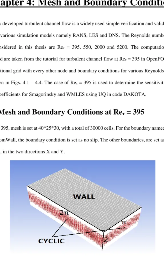
Chapter 4: Mesh and Boundary Conditions

The fully developed turbulent channel flow is a widely used simple verification and validation test case for various simulation models namely RANS, LES and DNS. The Reynolds numbers of the flow considered in this thesis are Reτ = 395, 550, 2000 and 5200. The computational grids

employed are taken from the tutorial for turbulent channel flow at Reτ = 395 in OpenFOAM. The

computational grid with every other node and boundary conditions for various Reynolds numbers

are shown in Figs. 4.1 – 4.4. The case of Reτ = 395 is used to determine the sensitivities of the

model coefficients for Smagorinsky and WMLES using UQ in code DAKOTA.

4.1 Mesh and Boundary Conditions at Re

τ

= 395

At Reτ = 395, mesh is set at 40*25*30, with a total of 30000 cells. For the boundary named topWall

and bottomWall, the boundary condition is set as no slip. The other boundaries, are set as periodic or cyclic, in the two directions X and Y.

18

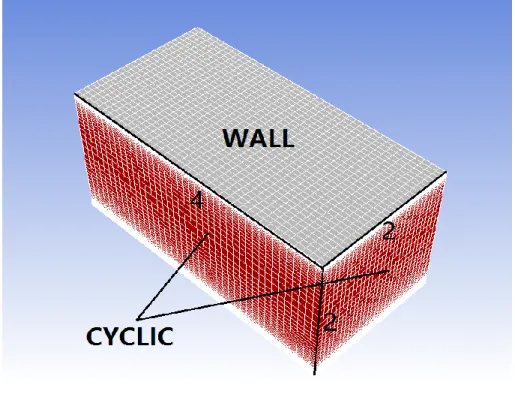
4.2 Mesh and Boundary Conditions at Re

τ

= 550

Figure 4.2 Mesh and boundary conditions at Reτ = 550

At Reτ = 550, mesh is set at 40*50*30, with a total of 60000 cells. For the boundary named topWall

and bottomWall, the boundary condition is set as no slip. The other boundaries, are set as periodic or cyclic, in the two directions X and Y.

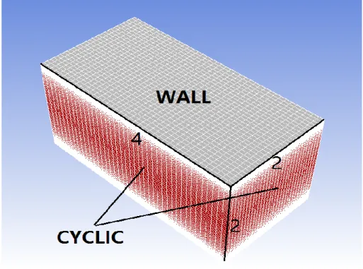
4.3 Mesh and Boundary Conditions at Re

τ

= 2000

At Reτ = 2000, mesh is set at 40*100*30, with a total of 120000 cells. For the boundary named

topWall and bottomWall, the boundary condition is set as no slip. The other boundaries, are set as periodic or cyclic, in the two directions X and Y.

19

Figure 4.3 Mesh and boundary conditions at Reτ = 2000

4.4 Mesh and Boundary Conditions at Re

τ

= 5200

At Reτ = 5200, mesh is set at 80*100*60, with a total of 480000 cells. For the boundary named

topWall and bottomWall, the boundary condition is set as no slip. The other boundaries, are set as periodic or cyclic, in the two directions X and Y.

20

21

Chapter 5: UQ of Skin Friction Coefficient

with Smagorinsky and WMLES models

5.1 Sobol Indices for Skin Friction Coefficient

Tables describe the sensitivity of the LES turbulence models (Smagorinsky and WMLES) to changes in the model’s closure coefficients for the channel flow at different Reynolds numbers. OpenFOAM is used as the flow solver and Sobol indices, are computed using SANDIA National Labs DAKOTA software; Sobol indices are used to rank the influence of each model coefficient. Tables 5.1 – 5.3 show the sensitivity analysis results obtained from OpenFOAM for the skin friction coefficients at Reτ = 550, Reτ = 2000 and Reτ = 5200.

5.1.1 Sobol Indices for Re

τ

= 550

Table 5.1 Sobol Indices for the skin friction coefficient from OpenFOAM when Reτ = 550.

Smagorinsky WMLES

Coefficient Sobol Index Coefficient Sobol Index

𝑪_𝒌 0.693 𝑪_𝒌 0.380

𝑪𝜺 0.307 𝑪𝜺 0.302

𝜿 0.216

𝑨+ _0.102

As shown in Table 5.1, for Reτ = 550, in Smagorinsky model there are only two coefficients.

Between 𝐶_𝑘 and 𝐶_𝜀, the most significant coefficient is obviously 𝐶_𝑘, which has a Sobol index of 0.693; 𝐶_𝜀 has a index of 0.307. 𝐶_𝑘 also plays an important role in case of WMLES model. However,

22

to be very important in WMLES model at Reτ = 550, the sum of their Sobol Indices is only 0.318,

less than that of 𝐶_𝑘.

5.1.2 Sobol Indices for Re

τ

= 2000

Table 5.2 Sobol indices for the skin friction coefficient from OpenFOAM when Reτ = 2000

Smagorinsky WMLES

Coefficient Sobol Index Coefficient Sobol Index

𝑪_𝒌 0.543 𝑪_𝒌 0.104

𝑪_𝜺 0.457 𝑪_𝜺 0.077

𝜿 0.501

𝑨+ _0.318

As shown in Table 5.2, at Reτ = 2000, in case of Smagorinsky model, the most significant

coefficient is 𝐶_𝑘, although it begins to decrease compared to Reτ = 550 case, its significance is still

higher than that of 𝐶_𝜀. In case of WMLES model, the coefficient which contributes most to the

skin friction coefficient is 𝜅 with Sobol index of 0.501. 𝐴+also has an index of 0.318. The Sobol indices are completely different with case compared to those for Reτ = 550. 𝐶𝜀 and 𝐶𝑘 become less

important in WMLES model when Reτ = 2000.

5.1.3 Sobol Indices for Re

τ

= 5200

At Reτ = 5200, in Smagorinsky model, the most significant coefficient is 𝐶_𝜀, with a Sobol index of

0.652, completely opposite to the situation for Reτ = 550 case. In case of WMLES model, the

coefficient which contributes most to the skin friction coefficient is 𝐴+. 𝜅 also has an important influence on the result with a Sobol index of 0.339. 𝐶_𝜀 and 𝐶_𝑘 become least important most in

23

Table 5.3 Sobol indices for the skin friction coefficient from OpenFOAM when Reτ = 5200.

Smagorinsky WMLES

Coefficient Sobol Index Coefficient Sobol Index

𝑪𝒌 0.348 𝑪𝒌 0.068

𝑪_𝜺 0.652 𝑪_𝜺 0.107

𝜿 0.339

𝑨+ _0.486

5.2 Change in Skin Friction Coefficient with Change in

Coefficients of Smagorinsky and WMLES model

5.2.1 Change in Skin Friction Coefficient in Smagorinsky Model

Table 5.4 – 5.7 show two change in skin-friction by changing the coefficients (decreasing and increasing by 10% from the standard value) in Smagorinsky and WMLES models.

Table 5.4 Sobol indices at various Reτ for Smagorinsky model by decreasing the coefficients by 10%.

Coefficient

Smagorinsky

Reτ = 550 Reτ = 2000 Reτ = 5200

𝐶𝑓 %change 𝐶𝑓 %change 𝐶𝑓 %change

𝑪_𝒌− 4.456E-03 -1.81% 3.318E-03 -1.31% 2.804E-03 -1.02%

𝑪_𝜺− 4.587E-03 1.08% 3.399E-03 1.07% 2.898E-03 2.29%

Table 5.5 Sobol indices of for various Reτ for Smagorinsky model with increasing coefficients by 10%.

Coefficient

Smagorinsky

Reτ = 550 Reτ = 2000 Reτ = 5200

𝐶_𝑓 %change 𝐶_𝑓 %change 𝐶_𝑓 %change

𝑪𝒌+ 4.644E-03 2.33% 3.435E-03 2.17% 2.869E-03 1.27%

24

It can be seen from Table 5.4 – 5.7 that in case of Smagorinsky model, as coefficients increased by 10%, skin friction coefficient increases with 𝐶_𝑘, but decreases with 𝐶_𝜀. Similar situation occurs when the coefficients decrease by 10%.

5.2.2 Change in Skin Friction Coefficient in WMLES Model

Table 5.6 Sobol indices at various Reτ for WMLES model by decreasing the coefficients by 10%.

Coefficient

WMLES

Reτ = 550 Reτ = 2000 Reτ = 5200

𝐶_𝑓 %change 𝐶_𝑓 %change 𝐶_𝑓 %change

𝑪𝒌− 4.410E-03 -2.82% 3.331E-03 -0.92% 2.810E-03 -0.81%

𝑪_𝜺− 4.642E-03 2.29% 3.383E-03 0.62% 2.869E-03 1.27%

𝜿− 4.459E-03 -1.74% 3.303E-03 -1.75% 2.782E-03 -1.80%

𝑨+

− 4.507E-03 -0.68% 3.312E-03 -1.49% 2.726E-03 -3.78%

Table 5.7 Sobol indices at various Reτ for WMLES model by increasing coefficients by 10%

Coefficient

WMLES

Reτ = 550 Reτ = 2000 Reτ = 5200

𝐶𝑓 %change 𝐶𝑓 %change 𝐶𝑓 %change

𝑪_𝒌+ 4.646E-03 2.38% 3.387E-03 0.71% 2.861E-03 0.99%

𝑪_𝜺+ 4.451E-03 -1.92% 3.346E-03 -0.51% 2.791E-03 -1.48%

𝜿+ 4.610E-03 1.59% 3.450E-03 2.59% 2.899E-03 2.33%

𝑨+

+ 4.587E-03 1.08% 3.427E-03 1.90% 2.923E-03 3.17%

In case of WMLES model, it can be seen from Table 5.6 and 5.7 that when the coefficients increase by 10%, skin friction coefficient increases with 𝐶_𝒌, 𝜅 and 𝐴+ but decreases with 𝐶_𝜀. Similar situation occurs when the coefficients decrease by 10%.

25

5.3 Conclusions

Several interesting conclusions can be made from the result in section 5.2.

First, in case of Smagorinsky model, the sensitivity of 𝐶_𝑘 decreases and that of 𝐶_𝜀 becomes more

important, with increasing Reynolds number. Also, as the Reynolds number becomes larger, 𝐶_𝑘

and 𝐶_𝜀 reverse the role in terms of importance.

In case of WMLES model, sensitivity of different model coefficients on the skin-friction

coefficient change with Reynolds number. With increase in Reynolds number, importance of 𝐶_𝑘

and 𝐶𝜀 on the skin friction coefficient becomes less and less, and that of 𝜅 and 𝐴+ becomes more. Table 5.8 and 5.9 show the Sobol indices in two model coefficients in their overlapping region and variation in their value with Reynolds number.

Table 5.8 Sobol indices of a combination of two model coefficients for the skin friction coefficient from

OpenFOAM for Smagorinsky model

Smagorinsky

Coefficients Combination Sobol indices in the overlapping region

Reτ = 550 Reτ = 2000 Reτ = 5200

𝑪𝜺 & 𝑪𝒌 1.97E-01 2.03E-02 6.75E-03

Table 5.9 Sobol indices of a combination of two model coefficients for the skin friction coefficient from

OpenFOAM for WMLES model

WMLES

Coefficients Combination Sobol indices in the overlapping region

Reτ = 550 Reτ = 2000 Reτ = 5200

𝑪𝜺 & 𝑪𝒌 1.80E-01 2.71E-03 2.29E-03

𝑪_𝜺 & 𝜿 2.86E-01 4.94E-02 9.10E-03

𝜿 & 𝑪𝒌 2.20E-02 1.07E-02 1.25E-04

26 𝑨+ _{& 𝑪}

𝒌 1.30E-01 1.30E-02 4.54E-02

27

Chapter 6: UQ of Mean Velocity Profiles

from Smagorinsky and WMLES Model

In this chapter, uncertainty quantification (UQ) of velocity profiles in the channel obtained using the Smagorinsky model and WMLES model is conducted. It will be shown how the model coefficients can influence the velocity profile at various Reynolds numbers. By changing the model coefficients, the sensitivity of the coefficients on the global velocity profile is also shown.

6.1 UQ of Velocity Profile when Re

τ

= 550

6.1.1 UQ of Velocity Profile from Smagorinsky Model

As shown in Fig.6.1, at Reτ = 550, for Smagorinsky model, the Sobol index of 𝐶_𝑘 begins around

0.748 and that of 𝐶_𝜀 around 0.252. Sobol index of 𝐶_𝑘 reaches maximum value of 0.997 when y+ is 100. After that, the Sobol index of 𝐶_𝑘 decreases, and remains near 0.7 when y+ _{is between 175 and}

350. When distance from the wall becomes large, 𝐶𝑘 again dominates the change in and finally

becomes 0.988 in the middle of the channel.

𝐶_𝑘 can be regarded as the most significant coefficient in this case. If a more accurate prediction of

velocity is required using the LES Smagorinsky model, the most effective way is to change 𝐶_𝑘.

After several computational tests, it can be found that as 𝐶𝑘is increased, velocity profile gets closer to the DNS data. As shown in Fig. 6.2, red lines and green lines are the velocity profiles when the that value of 𝐶_𝑘increased by 20% and 10%, respectively with respect to their original value.

28

Figure 6.1 Sobol indices along the y direction for Smagorinsky model at Reτ = 550

0 0.2 0.4 0.6 0.8 1 1 10 100 Sobol Indices y+ Ck Ce

29

Figure 6.2 Comparison of velocity profiles obtained by increasing 𝑪_𝒌 by 20% and 10% for Smagorinsky model with DNS data atReτ = 550

6.1.2 UQ of Velocity Profiles for WMLES Model

As shown in Fig. 6.3, The situation is more complex compared to that the situation for Smagorinsky model since there are four model coefficients. 𝜅 ranks first when y+ begins to increase. Before y+ reaches 100, 𝜅 is always the most influential coefficient in affecting the mean velocity. As y+ becomes greater than 30, which is the log-law region, the coefficient 𝐶𝜀 begins to

increase and becomes the most significant coefficient to affect the mean velocity after y+ = 100.

However, when y+ _{is between 150 and 350, it can be seen from this figure that 𝐶}

𝑘 most influences the mean velocity. Finally, near the middle of the channel, 𝐴+ contributes most to the mean velocity profile.

𝜅 is the most important coefficient in the buffer layer. After several computational tests, it was found that decreasing 𝜅 is the best way to make the velocity profile closer to the DNS data. In Fig.

0.1 1 10 100 0 5 10 15 20 25 y+ u+ Ck+20% Ck+10% Smagorinsky model DNS

30

6.4, it can be seen that by decreasing 𝜅 by 20% and 10%, velocity profile becomes closer to the

DNS data.

Thus, it can be inferred that y+ has an enormous influence on the value of Sobol indices that affect the velocity profile, and therefore, various coefficients should be modified to get the best LES velocity profile compared to the DNS data.

Figure 6.3 Sobol indices along the y direction for WMLES model at Reτ = 550

0 0.1 0.2 0.3 0.4 0.5 1 10 100 Sobol Indices y+ Ck Ce kappa A+

31

Figure 6.4 Comparison of velocity profile obtained by decreasing 𝜅 by 20% and 10% for WMLES model with DNS data at Reτ = 550

6.2 UQ of Velocity Profile when Re

τ

= 2000

6.2.1 UQ of Velocity Profile from Smagorinsky Model

At Reτ = 2000, it can be seen from Fig. 6.5 that the situation is similar to the when Reτ = 550 case.

Along the y direction in the buffer layer (5 < y+ _{< 30), 𝑪}

𝒌 is the most significant coefficient, although 𝑪𝜺 become slightly more important than 𝑪𝒌 for 200 < y+ < 300, however in most y+ range Sobol index of 𝑪𝒌 is larger. It can also be seen that after y+ > 30, in log-law region, Sobol index of 𝑪_𝒌decreases. When y+ > 1000, Sobol indices of both coefficients become chaotic and irregular. It is due to the fact that when y+ > 1000, the flow is in law of wake region where large scale turbulent eddies dominate. 0.1 1 10 100 0 5 10 15 20 25 y+ u+

32

Similar to the situation when Reτ = 550, 𝐶_𝑘is the most important coefficient. As shown in Fig. 6.6,

𝐶_𝑘 is increased by 20% (red line) and 10% (green line) and 𝐶_𝑘 with 20% increase provides a closer agreement between the simulation and DNS data.

Figure 6.5 Sobol indices along the y direction for Smagorinsky model at Reτ = 2000

0 0.2 0.4 0.6 0.8 1 1 10 100 1000 Sobol Indices y+ Ck Ce

33

Figure 6.6 Comparison of velocity profiles obtained by increasing 𝐶_𝑘 by 20% and 10% for Smagorinsky model with DNS data at Reτ = 2000

6.2.2 UQ of Velocity Profile for WMLES Model

For WMLES model at Reτ = 2000, Sobol indices are shown in Fig. 6.7. This figure shows that 𝐶_𝑘

is the most influential coefficient in the viscous sublayer, but immediately decreases after that. 𝜅 and 𝐴+ don’t contribute much in this situation and keep a low value. 𝐶_𝜀 becomes increasingly more important in the log-law region and exceed the Sobol index of 𝐶_𝑘 when y+ _{is around 700. For}

y+ _{> 1000, no significant information as the model coefficients can be obtained.}

𝐶_𝑘 is chosen as the most significant model coefficient and when it increases, velocity profile becomes closer to DNS data shown in Fig. 6.8. Red and green curves for velocity profile represent increase in 𝐶𝑘 of 20% and 10%, respectively.

0.1 1 10 100 1000 0 5 10 15 20 25 30 y+ u+ Ck+20% Ck+10% Smagorinsky model DNS

34

Figure 6.7 Sobol indices along the y direction for WMLES model at Reτ = 2000

0 0.1 0.2 0.3 0.4 0.5 0.6 0.7 0.8 0.9 1 10 100 1000 Sobol indices y+ Ck Ce kappa A+

35

Figure 6.8 Comparison of velocity profiles obtained by increasing 𝜅 by 20% and 10% for WMLES model with DNS data at Reτ = 2000

6.3 UQ of Velocity Profile when Re

τ

= 5200

6.3.1 UQ of Velocity Profile from Smagorinsky Model

For Reτ = 5200, using the Smagorinsky model, the trend in Sobol indices is almost the same as in

Fig. 6.5 for Reτ = 2000. Sobol indices of 𝑪_𝒌 begin to decrease in the log-law layer and remain

around 0.75 until y+ reaches 1000. However, 𝑪_𝒌has the most influence on the mean velocity profile up to y+ > 1000.

Fig. 6.10 shows the comparison of the velocity profiles with the DNS data when 𝑪_𝒌is increased

by 20% (red line) and 10% (green line); The red line with 20% increase in 𝑪_𝒌 is closer to the DNS

data. 0.1 1 10 100 1000 0 5 10 15 20 25 30 y+ u+ Ck+20% Ck+10% WMLES mdoel DNS

36

Figure 6.9 Sobol indices along the y direction for Smagorinsky model at Reτ = 5200

0 0.2 0.4 0.6 0.8 1 1 10 100 1000 Sobol Indices y+ Ck Ce

37

Figure 6.10 Comparison of velocity profiles obtained by increasing 𝑪_𝒌 by 20% and 10% for Smagorinsky model with DNS data at Reτ = 5200

6.3.2 UQ of Velocity Profile for WMLES Model

Fig. 6.11 shows that Sobol indices of WMLES model when Reτ = 5200. In the viscous sublayer (0

< y+ _{< 5), 𝜿 ranks first with value of 0.93. When y}+ _{increases, and goes into the buffer layer, Sobol}

index of 𝜿 decreases and 𝑪𝜺increases. Finally, 𝑪𝜺dominates the influence on the mean velocity profile after the log-law region, until the outer layer. In the velocity defect layer, the Sobol indices become chaotic.

In this case, 𝑪𝜺contributes most to the velocity profile. Fig. 6.12 shows the comparison of velocity

profile with DNS data when𝑪_𝜺decreases by 20% (red line) and 10% (green line); The red line

with 20% increase in 𝑪_𝜺 shows closer agreement with the DNS data.

0.1 1 10 100 1000 0 5 10 15 20 25 30 y+ u+ Ck+20% Ck+10% Smagorinsky model DNS

38

Figure 6.11 Sobol indices along the y direction for WMLES model at Reτ = 5200

0 0.2 0.4 0.6 0.8 1 1 10 100 1000 Sobol Indices y+ Ck Ce kappa A+

39

Figure 6.12 Comparison of velocity profiles obtained by decreasing 𝑪𝜺by 20% and 10% for WMLES model with

DNS data at Reτ = 5200 0.1 1 10 100 1000 0 5 10 15 20 25 30 y+ u+

40

Chapter 7: Conclusions

In this thesis, an uncertainty quantification (UQ) methodology has been successfully implemented in OpenFOAM. UQ studies focusing on the closure coefficients of two LES models for tuebulent flow in a channel are performed. Two LES turbulence models considered are the Smagorinsky model and the Wall-Modeled Large Eddy Simulation (WMLES) model. Sobol Indices are used to rank the contributions of each model coefficient to total model uncertainty.

First, the LES computations of turbulent flow in the channel were validated by comparing the velocity profile obtained using the original Smagorinsky model with that obtained by the modified

Smagorinsky model. Computations were then performed of Reynolds number Reτ = 395, 550, 2000

and 5200 using the Smagorinsky model and WMLES model. It was found that WMLES results were closer to the DNS data compared to Smagorinsky model results.

Uncertainty quantification due to various model coefficients was illustrated by computing the Sobol indices for skin friction coefficient and the velocity profile. In case of skin friction

coefficient for the Smagorinsky model, Sobol index of model coefficient 𝐶_𝑘increases and that of

𝐶_𝜀 decreases with increase in Reynolds number. For WMLES model, as the Reynolds number

increases, the dominant influence of𝐶𝑘 and 𝐶𝜀 is replaced by 𝜅 and 𝐴+. For the velocity profile, in case of the Smagorinsky model, 𝐶𝑘 was found to be the most significant coefficient at all Reynolds numbers. However for the WMLES model, 𝜅 , 𝐶_𝑘and 𝐶_𝜀 were the most significant coefficient for Reτ = 550, 2000, 5200 respectively. It was shown that a closer agreement in velocity

41

Chapter 8: Future Work

Influence of combined variation of various model coefficients on the mean velocity profile in channel should be evaluated to further improve the LES results compared to DNS data. It will require the global UQ analysis in multi-dimensional space.

UQ analysis should also be conducted for LES computation of turbulent boundary layer on a flat plate using both the Smagorinsky and WMLES models. However, to perform the UQ analysis for this case at high Reynolds numbers requires enormous computational resources.

42

References

[1] J. Smagorinsky. General circulation experiments with the primitive equations I. the basic experiment. Mon. Weather Rev., 91 (3) (1963), pp. 99–164

[2] Breden D. Tracey. Machine learning for model uncertainties in turbulence models and monte

carlo integral approximation. PhD dissertation, Stanford University, June 2015.

[3] David W Levy, Thomas Zickuhr, John Vassberg, Shreekant Agrawal, Richard A Wahls, Shahyer Pirzadeh, and Mchael J Hemsch. Data summary from the first AIAA computational fluid dynamics drag prediction workshop. Journal of Aircraft, 40(5):875-882, 2003.

[4] Kelly R laflin, Steven M Klausmeyer, Tom Zickuhr, John C Vassberg, Richard A Wahls, Joseph H Morrison, Olaf P Brodersen, Mark E Rakowitz, Edward N Tinoco, and Jean-Luc Godard. Data summary from second AIAA computational fluid dynamics drag prediction workshop. Journal of Aircraft, 4295):1165-1178, 2005.

[5] John C Vassberg, Edward N Tinoco, Mori Mani, David Levy, Tom Zickuhr, Dimitri J Mavriplis, Richard A Wahls, Joseph H Morrison, Olaf P Brodersen, Bernhard Eisfield, et al. Comparison of NTF experimental data with CFD predictions from the third AIAA CFD drag prediction workshop. AIAA paper, 2008-5918, 2008.

[6] John C Vassberg, Edward N Tinoco, Mori Mani, Ben Rider, Tom Zickuhr, David W Levy, Olaf P Brodersen, Bernhard Eisfield, Simone Crippa, Richard A Wahls, et al. Sumaary of the fourth AIAA CFD drag prediction workshop, AIAA paper, 2010-4547, 2010

[7] David W Levy, Kelly R laflin, Edward N Tinoco, John C Vassberg, Mori Mani, Ben Rider, Chris Rumsey, Richard A Wahls, Joseph H Morrison, Olaf P Brodersen, et al. Summary of data from the fifth AIA CFD drag prediction worshop, 2013-46, 2013.

[8] N. Wiener. The homogeneous chaos. American Journal of Mathematics，60(4):897-936, 1938.

[9] D. Xiu and G. E. Karniadakis. Modeling uncertainty in row simulations via generalized polynomial chaos. Journal of Computational Physics, 187(1):137-167, May 2003.

[10] J. B. Pleming D. S. Riha C. Waldhart L. Huyse, A. R. Bonivtch and B. H. Thacker.

Verification of stochastic solutions using polynomial chaos expansions, AIAA 2006-1994. In 47th

AIAA/ASME/ASCE/AHS/ASC Structures, Structural Dynamics, and Material Conference, Newport, RI, May 2006.

[11] M. S. Eldred, C. G. Webster, and P. G. Constantine. Evaluation of non-intrusive approaches

for Wiener-Askey generalized polynomial chaos, AIAA 2008-1892. In 10th AIAA

43

[12] S. Hosder and R. W. Walters. Non-intrusive polynomial chaos methods for uncertainty quantification in fluids dynamics, AIAA 2010-129. In 48th AIAA Aerospace Sciences Meeting Including the New Horizons Forum and Aerospace Exposition, Orlando, FL, January 2010. [13] R. W. Walters and L. Huyse. Uncertainty analysis for fluid mechanics with applications. Technical report, ICASE 2002-1, NASA/CR-2002-211449, NASA Langley Research Center, Hampton, VA, 2002.

[14] H. N. Najm. Uncertainty quantification and polynomial chaos techniques in computational fluid dynamics. Annual Review of Fluid Mechanics, 41:35-52, January 2009.

[15] https://www.cfd-online.com/Forums/openfoam-solving/57889-les-turbulent-channel-flows.html

44

Vita

Zuoxian Hou

Degrees M.S. Mechanical Engineering, Washington University in St. Louis, May

2017

B.S. Mechanical Engineering, Xi’an JiaoTong University, June 2015