Forecasting Aggregates by Disaggregates

Forecasting Aggregates by Disaggregates

David F. Hendry and Kirstin Hubrich∗ Department of Economics, Oxford University and Research Department, European Central Bank.

January, 2005

Abstract

We explore whether forecasting an aggregate variable using information on its disaggregate components can improve the prediction mean squared error over forecasting the disaggregates and aggregating those forecasts, or using only aggregate information in forecasting the aggregate. An implica-tion of a theory of predicimplica-tion is that the first should outperform the alternative methods to forecasting the aggregate in population. However, forecast mod-els are based on sample information. The data generation process and the forecast model selected might differ. We show how changes in collinearity between regressors affect the bias-variance trade-off in model selection and how the criterion used to select variables in the forecasting model affects forecast accuracy. We investigate why forecasting the aggregate using in-formation on its disaggregate components improves forecast accuracy of the aggregate forecast of Euro area inflation in some situations, but not in others. The empirical evidence on Euro-zone inflation forecasts suggests that more information can help, more so by including macroeconomic variables than disaggregate components.

JEL: C32, C51, C53, E31

KEYWORDS: Disaggregate information, predictability, forecast model selection, VAR, factor models

∗

Preliminary and incomplete: please do not cite without the authors’ permission. We thank seminar participants at Humboldt University and the Free University, Berlin, participants of the ESF-EMM conference, Sardinia, and the CEPR/EABCN workshop on forecasting combination, Brussels, in particular Graham Elliott and Lutz Kilian, for useful comments. Financial support from the ESRC under grant RES 051 270035 is gratefully acknowledged. The views expressed in this paper are not necessarily those of the European Central Bank.

1

Introduction

Forecasts of marcoeconomic aggregates are used by the private sector, governmen-tal and international institutions as well as central banks. Recently there has been renewed interest in the effect of contemporaneous aggregation in forecasting. For example, one issue has been the potential improvement in forecast accuracy de-livered by forecasting the component indices and aggregating such forecasts, as against simply forecasting the aggregate itself.1 The theoretical literature shows that aggregating component forecasts improves over directly forecasting the ag-gregate if the data generating process is known. If the data generating process is not known and the model has to be estimated, it depends on the unknown data gen-erating process whether the disaggregated approach improves the accuracy of the aggregate forecast. It might be preferable to forecast the aggregate directly. Since in practice the data generating process is not known, it remains an empirical ques-tion whether aggregating forecasts of disaggregates improves forecast accuracy of the aggregate of interest. For example, the results in Hubrich (2004) indicate that aggregating forecasts by component does not necessarily help to forecast year-on-year Eurozone inflation twelve months ahead.

In this paper, we suggest an alternative use of disaggregate information to fore-cast the aggregate variable of interest, that is to include the disaggregate informa-tion or disaggregate variables in the model for the aggregate as opposed to fore-casting the disaggregate variables separately and aggregating those forecasts.

We show that disaggregating elements of the information setIT−1 into their

components cannot lower predictability of a given aggregatey_T. We focus on disaggregation across variables (such as sub-indices of a price measure). Disag-gregation may also be considered across space (e.g., regions of an economy), time (higher frequencies), or all of these. The predictability concept considered in this paper concerns a property in population of the variable of interest in relation to an information set. A related predictability concept is discussed by Diebold & Kilian (2001). Whereas that paper considers measuring predictability of different variables based on one information set, we investigate predictability of the same variable based on different information sets. In contrast to predictability as a prop-erty in population, we use ’forecastability’ to refer to the improvement in forecast accuracy related to the sample information given the unconditional moments of a

1

See e.g. Espasa, Senra & Albacete (2002), Hubrich (2004) and Benalal, Diaz del Hoyo, Lan-dau, Roma & Skudelny (2004); see also Fair & Shiller (1990) for a related analysis for US GNP). Contributions to the theoretical literature on aggregation versus disaggregation in forecasting can be found in e.g. Grunfeld & Griliches (1960), Kohn (1982), L ¨utkepohl (1984, 1987), Pesaran, Pierse & Kumar (1989), Van Garderen, Lee & Pesaran (2000); see also L ¨utkepohl (2004) for a recent review on forecasting aggregated processes by VARMA models.

variable. Potential misspecification of the forecast model due to model selection and estimation uncertainty as well as data measurement errors and structural breaks will affect the accuracy of the resulting forecast and help to explain why theoret-ical results on predictability are not confirmed in empirtheoret-ical applications (see also Hendry (2004) and Clements & Hendry (2004a)).

In contrast to most previous papers on disaggregation in forecasting that are set up in a VAR framework, our proposal for including disaggregate variables in the aggregate model, gives rise to a classical model selection problem. We anal-yse model selection and estimation in the conditional model. We condition on We particularly focus on model selection for forecasting, the role of model misspeci-fication in the forecast period and changes in collinearity between regressors. The degree of misspecification, i.e. the deviation of the forecast model from the true data generating process in the forecast period, is not known in practice. Although the predictability theory provides a useful guide for forecasting, we need to empir-ically investigate the usefulness of different methods of model selection to include disaggregate information for euro area inflation. Thereby we extend the results in Hubrich (2004) and relate our empirical findings to the analytical results presented in the previous sections.

The paper is organised as follows. First, section 2 briefly reviews the notion of (un-)predictability and its properties most relevant to our subsequent analysis. Then we show that adding lagged information on disaggregates to a model of an aggregate must improve predictability. However, an improvement in predictabil-ity is a necessary, but not sufficient condition for an improvement in the forecast accuracy. In section 3, we investigate the effect of model selection and estimation uncertainty on the forecast accuracy in a conditional model with particular refer-ence to forecasting the aggregate when disaggregate information is included in the aggregate model. Section 4 notes an extension to dynamic forecasts for horizons larger than one. In section 5, we investigate in a simulated out-of-sample exper-iment whether adding lagged values of the sub-indices of the Harmonized Index of Consumer Prices (HICP) to a model of the aggregate improves the accuracy of forecasts of that aggregate relative to forecasting the aggregate HICP only using lagged aggregate information, or aggregating forecasts of those sub-indices. Sec-tion 6 concludes.

2

Improving predictability by disaggregation

In this section the notion of predictability and its properties most relevant to our subsequent analysis are reviewed first, before we address the issue of predictability

and disaggregation.2

2.1 Predictability and its properties

A non-degenerate vector random variable νt is unpredictable with respect to an

information setIt−1(which always includes the sigma-field generated by the past

ofνt) over a periodT = {1, . . . , T} if its conditional distributionDνt(νt|It−1)

equals its unconditionalDνt(νt):

Dνt(νt| It−1) =Dνt(νt) ∀t∈ T. (1)

Unpredictability, therefore, is a property ofνt in relation toIt−1 intrinsic toνt.

Predictability requires combinations withIt−1, as for example in:

yt=φt(It−1, νt) (2)

soytdepends on both the information set and the innovation component. Then:

Dyt(yt| It−1)=6 Dyt(yt) ∀t∈ T. (3)

The special case of (2) relevant here (after appropriate data transformations, such as logs) is predictability in mean:

yt=ft(It−1) +νt. (4)

Other cases of (2) which are potentially relevant are considered in Hendry (2004). In (4),ytis predictable in mean even ifνtis not as:

Et[yt| It−1] =ft(It−1)6=Et[yt],

in general. Since:

Vt[yt| It−1]<Vt[yt] when ft(It−1)6=0 (5)

predictability ensures a variance reduction.

Predictability is obviously relative to the information used. Given an informa-tion set,Jt−1 ⊂ It−1 when the process to be predicted isyt = ft(It−1) +νtas

in (4), less accurate predictions will result, but they will remain unbiased. Since Et[νt|It−1] =0:

Et[νt| Jt−1] =0, 2

The theory of economic forecasting in Clements & Hendry (1998, 1999) for non-stationary pro-cesses subject to structural breaks, where the forecasting model differs from the data generating mechanism, is rooted in the properties of (un-)predictability. Hendry (2004) considers the founda-tions of this predictability concept in more detail.

so that:

Et[yt| Jt−1] =Et[ft(It−1)| Jt−1] =gt(Jt−1),

say. Let et = yt−gt(Jt−1), then, providing Jt−1 is a proper information set

containing the history of the process:

Et[et| Jt−1] =0,

soetis a mean innovation with respect toJt−1.

However, as:

et= (ft(It−1)−gt(Jt−1)) +νt=wt−1+νt

(say) whereE[wt−1νt0] =0then:

Et[et| It−1] =ft(It−1)−Et[gt(Jt−1)| It−1] =ft(It−1)−gt(Jt−1)6=0.

As a consequence of this failure ofetto be an innovation with respect toIt−1:

E£ete0t ¤ = E£(νt+wt−1) (νt+wt−1)0 ¤ = E£νtνt0 ¤ +E£νtw0t−1 ¤ +E£wt−1νt0 ¤ +E£wt−1w0t−1 ¤ = E£νtνt0 ¤ +E£wt−1wt0−1 ¤ ≥ E£ν_tν_t0¤

where strict equality follows unlesswt−1 =0∀t.

Nevertheless, that predictions fromJt−1 remain unbiased on the reduced

in-formation set suggests that, by itself, incomplete inin-formation is not fatal to the forecasting enterprise.

In particular, disaggregating components of IT−1 into their elements cannot

lower predictability of a given aggregateyT, where such disaggregation may be

across space (e.g., regions of an economy), time (higher frequency), variables (such as sub-indices of a price measure), or all of these. These attributes sug-gest forecasting using general models to be a preferable strategy, and provide a formal basis for including as much information as possible, being potentially con-sistent with many-variable ‘factor forecasting’ (see e.g. Stock & Watson (2002), and Forni, Hallin, Lippi & Reichlin (2000)), and with the benefits claimed in the ‘pooling of forecasts’ literature (e.g., Clemen, 1989; Clements & Hendry, 2004b, for a recent theory). Although such results run counter to the common finding in forecasting competitions that ‘simple models do best’ (see e.g. Makridakis & Hi-bon, 2000; Allen & Fildes, 2001; Fildes & Ord, 2002), Clements & Hendry (2001) suggest that simplicity is confounded with robustness.

2.2 Predictability and disaggregation

The previous section concerns adding content to the information setJt−1to deliver

I_T−1. One form of adding information is via disaggregation of the target variable yT into its componentsyi,T althoughDyT+1(yT+1|·)remains the target of interest.

We consider only two components and a scalar process to illustrate the analysis, which clearly generalizes to many components and a vector process.

Consider a scalarytto be forecast, composed of:

y_T+1 =w_1,T+1y_1,T+1+w_2,T+1y_2,T+1 (6)

with the weightsw1,T+1andw2,T+1 = (1−w1,T+1)for each of the two

compo-nents. It may be thought that, when theyi,tthemselves depend in different ways on

the general information setIt−1, which by construction includes theσ–field

gen-erated by the past of theyi,t−j, predictability could be improved by forecasting the

disaggregates and aggregating those forecasts to obtain those foryT+1. However,

let:

ET+1[yi,T+1| IT] =δi,T0 +1IT (7)

which is the conditional expectation of each component yi,T+1 and hence is the

minimum mean-square error (MSE) predictor. Then, taking conditional expecta-tions in (6), aggregating the two terms in (7) deliversET+1[yT+1|IT]:

ET [yT+1| IT] = 2 X i=1 wi,T+1ET+1[yi,T+1| IT] = 2 X i=1

wi,T+1δi,T0 +1IT =λ0T+1IT (say).

By way of comparison, consider predictingyT+1 directly fromIT:

ET+1[yT+1 | IT] =φ0T+1IT, (8)

soφT+1 =λT+1with a prediction error:

y_T+1−E_T+1[y_T+1 | I_T] =v_T+1 (9)

which is unpredictable fromIT and hence nothing is lost predictingyT+1directly

instead of aggregating component predictions once the general information setIT

is used. In practice, if both the weightswi,T+1 and the coefficients of the

compo-nent modelsδ_i,T0 ₊₁change more than the coefficients of the aggregate modelλT+1,

forecasting the aggregate directly could well be more accurate than aggregating the component forecasts. Thus, the key issue in (say) aggregate inflation prediction is not predicting the component price changes, but including those components in the information setIT. This result implies that weights are not needed for aggregating

component forecasts, and also saves the additional effort of specifying disaggregate models for the components.

Including the components in the information setIT is quite distinct from

re-stricting information to lags of aggregate inflation, an information set we denote byJT. Then:

E_T+1[y_T+1| J_T] =ψ_T0 ₊₁J_T,

so that usingyT+1from (8) and (9) gives:

yT+1−ET+1[yT+1 | JT] =φT0 +1IT −ψ0T+1JT +vT+1, (10)

which must have largerMSEthan (9), since according to section 2.1, although the predictions based on IT and JT are both unbiased, the prediction based on the

smaller information setJT, here only including the lags of aggregate inflation and

no disaggregate information, is less accurate, and has a larger variance than the forecast based onIT. IfyT+1 was unpredictable from both information sets, i.e. ψ_T+1=φ_T+1 =0, then (9) and (10) would have equalMSE.

2.3 Example

Let the DGP be a vector autoregression of order one in the componentsyi,t: µ y1,t y2,t ¶ = µ π11 π12 π21 π22 ¶ µ y1,t−1 y2,t−1 ¶ + µ v1,t v2,t ¶ (11) whereE[vt] = 0, E[vtvt0] = Σv andE[vtv0s] = 0 for all s 6= t. Furthermore, yt=w1,ty1,t+ (1−w1,t)y2,t, as in a price index, where weights shift with value

shares, leading to:

yt = w1,t[(π11−π21)y1,t−1+ (π12−π22)y2,t−1] +π21y1,t−1+π22y2,t−1

+w1,tv1,t+ (1−w1,t)v2,t.

(12)

2.3.1 Disaggregate forecasting model: True disaggregate process known

The disaggregate forecasting model for known parameters is:

µ b y_1,T+1|T b y_2,T+1|T ¶ = µ π11 π12 π21 π22 ¶ µ y1,T y2,T ¶ , with: b y_T+1|T =w1,T+1yb1,T+1|T +w2,T+1yb2,T+1|T.

Thus, the forecast error from forecasting the disaggregate components and aggre-gating those forecasts is:

y_T+1−yb_T+1|T = w_1,T+1¡y_1,T+1−by_1,T+1|T¢+w_2,T+1¡y_2,T+1−yb_2,T+1|T¢

= w1,T+1v1,T+1+w2,T+1v2,T+1

(13) which is unpredictable, independent of whether the weights are known or not known.

2.3.2 Aggregate forecasting model with known parameters: True disaggre-gate process known

In contrast to the first example where the disaggregate forecasting model is fitted to the process, consider restricting the information set underlying the forecasting model to lags ofyt alone, with no disaggregates used. Furthermore, the true

ag-gregate process is assumed known so that the true parameters of the agag-gregate forecasting model are known to the forecaster. In the following, to simplify the presentation, it is assumed thatw1,t=w2,t= 1,3so thatyt=y1,t+y2,t. Then the

aggregateytbased on the true disaggregate process (11) can be represented by an

ARMA(2,1) process (for a proof see e.g. L¨utkepohl, 1987, Ch.4,1984a). The VAR in (11) can be written asΠ(L)yt=vt:

µ 1−π₁₁L −π₁₂L −π21L 1−π22L ¶ µ y_1,t y2,t ¶ = µ v_1,t v2,t ¶ . (14) Multiplying (14) by the adjointΠ(L)∗of the VAR operatorΠ(L)gives:

µ 1−a1−a2L2 0 0 1−a1−a2L2 ¶ µ y1,t y2,t ¶ = µ 1−π22L π12L π21L 1−π11L ¶ µ v1,t v2,t ¶ . (15) Furthermore, multiplying (15) by the vector of weightsF = (1,1)of the disaggre-gate components entails:

(1−a1L−a2L2)yt= (1−b1L)v1,t+ (1−b2L)v2,t (16)

witha1 =π11+π22,a2 =π12π21−π11π22,b1 =π21+π22andb2 =π12+π11. It

can be shown that the right-hand side of expression (16) is a process with an MA(1) representation, so that the aggregate process has an ARMA(2,1) representation:

(1−a1L−a2L2)yt= (1−γL)ut.4 3

Results are easily extended to the case of different and time-varying component weigths. 4

More generally, it has been shown in the literature that, if the disaggregate process follows a VARMA(p, q), the aggregate process follows an ARMA(p∗_{, q}∗

) process withp∗_{≤(n−m) + 1×p} andq∗≤(n−m)×p+qwithnbeing the number of variables in the system andmbeing the rank of the matrix of aggregation weights (see e.g. L ¨utkepohl, 1987, Ch.4).

The model in (16) is used as a forecasting model based on the information set restricted to the aggregate:

ˆ

y_T+1 =a₁y_T +a₂y_T−1+v_1,T+1−b₁v_1,T +v_2,T+1−b₂v_2,T (17) To derive the forecast error made, recall that the aggregate isyt=y1,t+y2,t. Then

(16) entails:

yt = a1y1,t−1+a2y1,t−2+a1y2,t−1+a2y2,t−2

+v1,t−b1v1,t−1+v2,t−b2v2,t−1 (18)

Since in this section, we have assumed thatw1,t=w2,t= 1for ease of exposition,

the disaggregate process in (11) simplifies to

yt= (π11+π21)y1,t−1+ (π12+π22)y2,t−1+v1,t+v2,t. (19)

Then the forecast error of the disaggregate process is given by the difference be-tween (19) and (18): b u_T+1|T = y_T+1−by_T+1|T = (π11+π21)y1,T −a1y1,T −a2y1,T−1 + (π12+π22)y2,T −a1y2,T −a2y2,T−1 +v1,T+1+v2,T+1−v1,T+1+b1v1,T −v2,T+1+b2v2,T = (π11−π22)y1,T −a2y1,T−1+ (π12−π11)y2,T −a2y2,T−1 +b1v1,T +b2v2,T

which will not be unpredictable in general. The entailed restrictions are of the following form5:

π21−π22 = 0 π12−π11 = 0

a₂ = −π₁₁π₂₂−π₁₂π₂₁= 0

These restrictions will usually not be fulfilled simultaneously, soutwill be

pre-dictable fromy1,t−iand/ory2,t−i(i= 1,2).

2.3.3 Aggregate forecasting model with unknown parameters: True disag-gregate process not known

Alternatively, consider again restricting the information set to lags ofyt with no

disaggregates used. In contrast to the previous example, the true disaggregate pro-cess is not known. Consequently, the aggregate propro-cess has to be approximated. A

5

(See e.g., L¨utkepohl, 1984, for the implied restrictions for equality of the aggregate and the disaggregate forecast model for a more general DGP).

further difference to the previous example is that we assume that the aggregate is a weighted average of the two disaggregates where the weights are allowed to vary across components and change over time.

We approximate (11) by an autoregression of the form:

y_t=ρy_t−1+u_t (20) where:

b

y_T+1|T =ρyb T.

Sinceyt=w1,ty1,t+ (1−w1,t)y2,t, (20) entails that:

y_t=ρw_1,t−1y_1,t−1+ρ(1−w_1,t−1)y_2,t−1+u_t. (21) Thus, the forecast errorubT+1|T from forecasting the true disaggregate process (11)

with an estimated AR(1) model is given by (12) minus (21):

b u_T+1|T = yT+1−byT+1|T = (w1,T+1[π11−π21] +π21−ρwb 1,T)y1,T + (w1,T+1[π12−π22] +π22−ρb(1−w1,T))y2,T +w_1,T+1v_1,T+1+ (1−w_1,T+1)v_2,T+1, (22)

which will not be unpredictable in general. Even for constant weights, the entailed restrictions are well known to be of the form:

w1(π11−π21−ρb) +π21 = 0 w₁(π₁₂−π₂₂+ρb) + (π₂₂−ρb) = 0

There is no reason to anticipate thatρbcan simultaneously satisfy both requirements (even less so with time-varying weights), souT+1will be predictable fromy1,T and y2,T, as in the previous example where the true aggregate process was known.

These results indicate that it should improve forecast accuracy to include disag-gregate information in the agdisag-gregate forecasting model. The additional difficulties in an actual forecast exercise of the choice of the information set, estimation of unknown parameters, unmodeled breaks, forecasting the weights, and data mea-surement errors that the forecaster faces, however, may be sufficiently large to offset the potential benefits. The role of estimation and model selection in a condi-tional model is considered analytically in the next section and is extended to a very simple dynamic forecasts in section 4.1. Section 5 presents an empirical analysis for forecasting euro-area inflation.

3

Model selection and estimation in a conditional model

When forecasting aggregates by disaggregates, the selection issue concerns retain-ing or omittretain-ing the disaggregates. First, a general framework is considered in this section to establish the role of model selection and estimation in a conditional model. Then we relate the discussion to the choice of a forecasting model for forecasting aggregates by disaggregates.

We first state our notation. Consider the conditional regression model:

y_t=β0x_t+ν_t where νt∼IN £

0, σ2_ν¤ (23)

withxt∼INk[µ,Σ](independent normal, meanµ, varianceΣ) independently of

{ν_t}.Then usingE[·]to denote an expectation: E£xtx0t

¤

=µµ0+Σ=Ω, (24) say withE[yt] = β0µ. The notation allows that one of the components ofxtis a

unit vector. For largeT, it is well known (see e.g., Hendry (1995) thatE[βb] = β

and: _√ T ³ b β−β ´ fa Nk £ 0, σ_ν2Ω−1¤, (25) so (V[·]denotes a variance): V h b β i 'σ_v2T−1Ω−1.

Forkregressors with estimated coefficients and a known outside-sample value ofx, denotedxT+1, a forecast can be based on:

b

yT+1 =βb0xT+1, (26)

when:

yT+1 =β0xT+1+νT+1, (27)

with a forecast error:

b νT+1 =yT+1−ybT+1 = ³ β−βb ´₀ xT+1+νT+1 (28)

so that its conditional mean-square forecast error (MSFE)is (lettingE[νT+1] = 0

andE£ν_T2₊₁¤=σ_ν2): M[bνT+1 |xT+1] =σv2+x0T+1V h b β i xT+1'σ2ν ¡ 1 +T−1x0_T+1Ω−1xT+1 ¢ . (29)

The unconditionalMSFEis obtained by taking the expectation of (29) over draw-ings ofxT+1from its distribution, mainly using (24), in which case, (29) simplifies

to the well-known formula:

M[νbT+1] =σν2 ¡

1 +T−1k¢. (30) Even in a constant parameter setting, to judge selection by (29) requires several aspects that do not seem to have been addressed, and are discussed below. First, what criteria should be used to judge the parsimony of the selected model? Re-searchers often use ‘statistical significance’, determined by the conventional rule that an observed t-statistic exceeds its 5% significance level, which is approxi-mately 2. To avoid having to consider signs, we translate that criterion intot2_b

βi ≥4

for the i-th variable. Since collinearity is likely to influence the observed t-value, we first analyze that issue, then consider the converse problem of omitting relevant variables, and finally combine these analyses to try to determine rules for model selection.

The assumptions underlying the conditionalMSFE(29) are quite strong since they imply parameter constancy. For an extensive analysis of such problems of different parameter values in the forecast regime the reader is referred to Clements & Hendry (1999).

3.1 Collinearity

Factorize the variance-covariance matrix Ωof the regressors xt in (25) as Ω =

H0_ΛHwhereH0_H=I

kandHxt=zt, so that:

E£z_tz0_t¤=Λ (31)

and:

yt=γ0zt+νt where γ =Hβ. (32)

Clearly, despite the transform,bγ ≡Hβband:

b

y_T+1=bγ0z_T+1 =βb0H0Hx_T+1 =βb0x_T+1,

so neither estimation nor forecasting are affected. Then:

x0_T+1Ω−1x_T+1 = x0_T+1¡H0ΛH¢−1x_T+1=x0_T+1H0Λ−1Hx_T+1 = z0_T+1Λ−1zT+1 = k X i=1 z2 i,T+1 λi . (33)

On average, (31) entails thatE[z_i,T2 ₊₁] =λi, and therefore, unconditionally: E£x0_T+1Ω−1xT+1 ¤ =E " _k X i=1 z2_i,T+1 λ_i # =k. (34)

Thus, substituting (34) in the unconditional value of (29) again simplifies to (30). That result shows that any ‘collinearity’ inxtis irrelevant to forecasting, so long as

the marginal process remains constant. Alternatively, the linear regression model

is invariant under linear, and therefore orthogonal transforms, as shown in (32), so collinearity is not an attribute of a model but only of a particular parameterization of that model.

3.1.1 Changes in collinearity in the forecast period

Whenβ stays constant, but the regressor variance-covariance matrixΩof the in-sample period changes toΩ∗ out-of-sample, so the mean square of the marginal processxT+1alters, withΛchanging toΛ∗then:

E " _k X i=1 z2 i,T+1 λi # = k X i=1 λ∗ i λi, (35)

so that the unconditionalMSFEis: M[bν_T+1]'σ_ν2 Ã 1 +T−1 k X i=1 λ∗ i λi ! . (36)

Changes in the magnitude of the eigenvalue of the least well determined βj,

corresponding to the smallestλj, will induce the biggest relative changes inM[νbT+1].

For example, let the smallestλj = 0.0001where the change is toλ∗j = 0.01which

remains small. Nevertheless,λ∗_j/λj = 100rather than unity, so a dramatic increase

in the MSFE arises from retaining that variable. 3.2 Mis-specification

Consider a model based on prior simplification which happens to exclude a re-gressor setx2,t, where we partitionx0t = (x01,t : x02,t)of dimensions k1 andk2

respectively, whenk1+k2 =k, leading to the forecast:

whereβ0 = (β0₁:β0₂)and: β₁ = Ã T X t=1 x1,tx01,t !−1Ã _T X t=1 x1,tyt ! . (38)

Without loss for an analysis of forecasting, we consider the case whereΩ=Λ, so that:6

β1,e =E[β1]'Λ−111ρ1y =β1+Λ−111Λ12β2=β1, (39)

whereρ1y =E[x1,tyt]. The forecast error resulting atT + 1isωT+1|T =yT+1− y_T+1|T so: ω_T+1|T =x₁0_,T+1¡β1−β1 ¢ +x0_2,T+1β2+ωT+1, (40) with expectation: E£ω_T+1|T |x_T+1¤=x0_1,T+1(β₁−β_1,e) +x0_2,T+1β₂ =x0_2,T+1β₂. (41) The forecast is systematically biased by x0_2,T+1β2. When x₂0_,T+1β2 ' x02,tβ2

∀t= 1, . . . , T, this bias is ‘absorbed by’, and reflected in, the in-sample estimates, so the forecastMSFE is close to that anticipated from the in-sample estimates.. However, ifx0_2,T+1differs markedly from in-sample values, then serious forecast errors could result. Therefore, in a non-constant parameter process a change even in the excluded variables matters for forecasting.

3.3 Mis-specification and collinearity

In this section, we derive the trade-off between the estimation costs from retaining a variable–leading to an increased forecast variance–and the increased bias due to mis-specification costs when a variable is incorrectly omitted. We consider a process with changing collinearity: note that under general linear transformations, that would become a non-constant parameter process.

The conditional variance of the forecast errorω_T+1|T due to the omission of a relevant variable is:

Eh¡ω_T+1|T −E£ω_T+1|T |xT+1 ¤¢₂ |xT+1 i =σ2_ω, (42) 6

A similar result holds under non-orthogonal regressors on replacing Λ22 below by Ω22 −

so using the factorizations from section 3.1, the conditionalMSFEis (tr denotes the trace): E h ω2_T+1|T |x_T+1 i = σ2_ω+tr©E£x_1,T+1x0_1,T+1¤V£β₁¤ª+β₂0E£x_2,T+1x0_2,T+1¤β₂ = σ2_ω à 1 +T−1 k1 X i=1 λ∗_i λi ! +β₂0Λ∗₂₂β2. (43)

Thus, the net costs of inappropriate exclusion are given by the last term relative to the ‘saving’ from not having the estimation cost of:

T−1 k X i=k1+1 λ∗_i λi.

This trade-off is central to selecting a particular specification from a class when the objective is forecasting, albeit that the future values of theλ∗_i are bound to be unknown, and is explored in more detail in section 4.

3.4 Adding disaggregates to forecast aggregates

Let yt denote the vector of n disaggregate prices with elements yi,t where we

illustrate using:

yt=Γyt−1+et (44)

as the DGP for the disaggregates. Letyt=ω0tytbe the aggregate price index with

weightsωt. Then pre-multiplying (44) byω0t: yt = ωt0Γyt−1+ωt0et=κω0t−1yt−1+

¡

ω_t0Γ−κω0_t−1¢yt−1+ωt0et

= κyt−1+ (φt−κωt−1)0yt−1+νt (45)

whereφt=Γωt. Thus, even if the DGP is (44) at the level of the components, an

aggregate model will be systematically improved by adding disaggregates only to the extent thatφt−κωt−1 =π is both constant, and elements contribute

substan-tively to the explanation.

To relate (45) to (23), letzt=ρ0xtbe an aggregate variable (such as a ‘factor’

component), so the analysis applies more widely than just price index aggregation, then (23) can be expressed as:7

y_t=κz_t+ (β−κρ)0x_t+u_t. (46)

7_{Even though (46) is perfectly collinear if the price index weights are unchanging, either any} component can be deleted or a PcGets model selection approach can be adopted (see Hendry & Krolzig, 2004) .

This requires thatβ is constant, and the choice of aggregate is a constant linear function ofxt. From (45), those conditions seem unlikely to be fulfilled when the

regressorsxtin (46) areyt−1 andztisyt−1 withρ = ωt−1. If so, the additional

role of disaggregate information over just the aggregate in (46) is represented by the extent to whichβ 6= κρ for each variable. This is similar to (45), with the added requirement of constancy ofπ.

Four distinct types of change can be distinguished in (45):

a) changes in the price index weightsωt−1 can be due to changes in expenditure

shares with constant correlations between the disaggregates;

b) changes in the second-moment matrix of the disaggregatesyt−1 (i.e., in the

re-gressor correlation structure) can change collinearity, inducing the effects noted in the previous section;

c) changes in the parametersφtof the disaggregates, so the role of the disaggregate

regressors is non-constant; and

d) changes in the autoregressive parameterκ.

All four potential shifts influence the decision of whether or not to include (or model) the disaggregates, and might hamper possible improvements in the forecast of the aggregateytfrom adding disaggregate variablesxi,tto a model with lags of

the aggregate already included. The first three of these shifts favour an aggregate model, and could do so even ifκis not constant. The selection issue in this con-text, therefore, concerns omitting or retaining the disaggregates, where the trade-off is between the impact of changing collinearity increasing forecast uncertainty as described in section 3.1.1, and the mis-specification costs of omitting relevant regressors considered in section 3.2. We evaluate that trade-off in a non-constant-parameter process in section 4, which establishes that for retention of disaggregate variables to be useful, the non-centralities of their squaredt-statistics in (45) must be greater than unity.

Given these results, we now consider the selection of a forecasting model.

4

Model selection for forecasting

The central issue of this paper is how to select a forecasting model given the con-siderations discussed above. When forecasting aggregates by disaggregates, the selection issue concerns retaining or omitting the disaggregates. First, a general framework is considered in this section to establish the role of model selection and estimation in a conditional model. Then we relate the discussion to the choice of a forecasting model for forecasting aggregates by disaggregates.

If all relevant variables were known and only those were included, and the observation to be forecast was a random draw from the same population as the

estimation sample, then (29) would correctly represent the resultingMSFE. If the ‘most-accurate forecast’ is defined by minimizingM[νbT+1|xT+1], then criteria for

trying to select that model can be determined. The central trade-off is between retaining or omitting variables that will improve the accuracy of the forecast mean, where retention will add to the forecast-error variance. Notice the deliberate use of the word ‘will’: even under the conditions stated here, (26) depends on the actual forecast origin (i.e.,xT+1). WhenxT+1 can differ markedly from any in-sample

observed value, model choice can differ from that conventionally supposed, and that issue is addressed below.

To relate theMSFE conditional onxT+1 in (43) to the unconditionalMSFE

in (36), we express the former in terms of the non-centralityτ_βj2 of the expected values of thet2-tests on theβ2,iin the DGP noting that:

β₂0Λ22β2 = k X i=k1+1

β_i2λi. (47)

Let the non-centralityτ_βj2 of the t2-tests on βj be expressed in terms of the true

parameters of the DGP: τ_βj2 = β 2 j P_T t=1x2j,t σ2 ω ' T β 2 jλj σ2 ω . (48)

From (43) and (48), the conditionalMSFEE[ω2

T+1|T|xT+1]from using only

the first set of regressorsx1,T+1 and omitting the secondx2,T+1 can be related to

the conditionalMSFEE[ωb2

T+1|T|xT+1]from using all the variables as:

E h ω2_T+1|T |xT+1 i ' σ_ω2  _{1 +T}−1 k1 X i=1 λ∗ i λi +T −1 k X j=k1+1 T β2 jλ∗j σ2 ω   = σ_ω2  _{1 +T}−1  Xk1 i=1 λ∗ i λi + k X j=k1+1 τ_βj2 λ ∗ j λj     = E h b ω_T2_+1|T |xT+1 i +σ 2 ω T k X j=k1+1 ³ τ_βj2 −1 ´_λ∗ j λj. (49)

For a simplified model to out-perform relative to the unrestricted requires that the averageτ_βj2 be less than unity for the omitted variables. In such a case, a selected model can out-perform the estimated DGP, as well as less parsimonious estimated

models. Omitting irrelevant variables (τ_βj2 = 0) is clearly sufficient to justify se-lecting the simplified model, but is not necessary. If there is no change in collinear-ity between the regressors in the forecast period in comparison with the in-sample period, i.e.,λ∗_j =λj, the cost-benefit traoff from (43) relative to (36) only

de-pends onPk_j=k1+1τ_βj2 relative tok2, but (49) reveals considerably more structure

to the choice. Indeed, when collinearity between the regressors is changing in the forecast period, e.g.,λ∗_j 6=λj, then the general formula in (49) is needed. Changes

in collinearity affect forecasts from both included and incorrectly-excluded vari-ables, so simply omitting highly collinear regressors is not a viable solution for selecting forecasting models.

For the illustrative case ofk2 = 1(which implies omitting one relevant

regres-sor) then the cost (or benefit) of omission is simply:

T−1σ_ω2¡τ_βk2 −1¢λ

∗

k

λk. (50)

If that variable is irrelevant, soτ_βk2 = 0, andλ∗_k> λkby a ratio of 100 (say), there

is a dramatic benefit to correct omission. Conversely, ifτ_βk2 = 2(as the symmetric case), an equally large loss occurs. However, the probability of retaining such a variable ont-testing also rises withτ_βk2 .

Notice that (49) is based on theτ_βk2 in the DGP, not the observedt2_βk=0 that happened to arise in-sample when estimating the model. Because thet2_βk=0have a sampling distribution even in the DGP, selecting those variables that happen to have observedt2_βk=0 values larger than unity will lower calculated MSFE (as shown above), but will not lower the trueMSFE unless they correspond toτ_βj2 > 1. Of course,τ2

βk is not observed, onlyt2βk=0. Under the null thatβk = 0, the squared t-test,t2_βk=0is: t2_βk=0 = T b β2 k P_T t=1x2k,t b σ2 ω ∼χ2₁(0), (51) so: E£t2_βk=0|τ_βk2 = 0¤=E£χ2₁(0)¤= 1.

Consequently (see () Johnson & Kotz, 1970):

E£t2_βk=0 |τ_βk2 6= 0¤'1 +τ_βk2 . (52)

Thus, although retention under the null would be 50% for a criterion wheret2_βk=0 >

1(only one tail of the distribution is relevant sinceβk6= 0can have either a positive

or a negative sign), the result in (52) suggests requiringt2_βk=0 >2as correct cut-off for retaining the associated variable.

In the present context, the disaggregate prices are inter-correlated, and seem to have changing collinearity, with weights that are also changing in the price index. In the empirical study, the weights in first year of the out-of-sample period change little, but change between 0% for processed food inflation up to almost 6.5% for energy inflation in 1999 over the previous (last in-sample period for 12 months ahead forecasts) year. Indeed, collinearity between components is changing from the in-sample to the out-of-sample period (and also over the forecast period).

Should some of the disaggregates have non-zero effects in (46), the costs of omitting them are the mis-specification effects in (49). We assume their net effects, after including the aggregate information, is not too large, sayτ_βk2 ≤9. Retaining a variable with a value ofτ_βk2 = 1 carries the same cost as omitting it, namely

T−1_σ2

ωλ∗k/λk: smallerτβk2 favour omission, larger favour retention. If the DGP

were by chance specified as the initial model, but tested in a conventional manner, then variables withτ_βk2 ₌₀ = 2would be retained on average (i.e., half the time) only if α = 0.16. Interestingly, that significance value is close to the implicit significance level of AIC whenT = 100for a range ofN (see Akaike (1973) and Campos, Hendry & Krolzig (2003)).

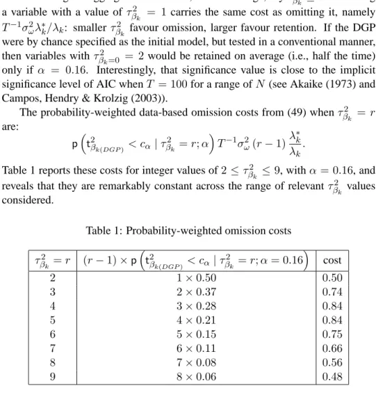
The probability-weighted data-based omission costs from (49) whenτ_βk2 = r are: p ³ t2_βk(DGP) < cα|τβk2 =r;α ´ T−1σ_ω2(r−1)λ∗k λk .

Table 1 reports these costs for integer values of2 ≤τ_βk2 ≤9, withα = 0.16, and reveals that they are remarkably constant across the range of relevantτ_βk2 values considered.

Table 1: Probability-weighted omission costs

τ2 βk =r (r−1)×p ³ t2 βk(DGP) < cα|τ 2 βk =r;α= 0.16 ´ cost 2 1×0.50 0.50 3 2×0.37 0.74 4 3×0.28 0.84 5 4×0.21 0.84 6 5×0.15 0.75 7 6×0.11 0.66 8 7×0.08 0.56 9 8×0.06 0.48

en-tering all the disaggregates at several lags, adventitious significance is likely: with

N irrelevant candidates and a significance level ofα, thenαN will be retained by chance. If such a loose significance level asα = 0.16 were used for a general model withN = 20,then3irrelevant variables would be retained on average, with costs ofP3_k=1σ_ω2T−1λ∗_k/λk. This corresponds roughly to the total effect for four

terms from table 1. A larger value ofα than 0.16 would lower the costs in table 1 and raise the retention rate for irrelevant variables, suggesting perhaps seeking equality for a givenN to minimize their total costs.

4.1 Dynamic forecasts

The analysis of open models, where some variables are not endogenized, is difficult primarily because the properties of the ‘explanatory’ variables are unspecified. In practice, for multi-step ahead forecasts, either those variables have to be forecasted ‘off-line’, which is reliant on untested strong exogeneity assumptions, endogenized for the forecasts risking ill-specified relationships, or multi-step estimation has to be adopted. The last of these is the subject of other research and will not be ad-dressed here: see inter alia Bhansali (2002) and Chevillon & Hendry (2004).

Moreover, the importance of parameter-estimation uncertainty is heavily de-pendent on the postulated nature of the DGP and the specific transformations of the variables to be forecast. Specifically, if the DGP is near non-stationary, but treated as stationary, and the horizon is relatively long compared to the estimation sample period available, then parameter-estimation uncertainty plays a fundamental role: see e.g., Stock (1996). The opposite extreme is when the DGP is stationary and a long estimation sample is available, in which case estimation becomes relatively ir-relevant as the horizon increases: see the results in Chong & Hendry (1986), noting the potential non-monotonicity of interval forecasts after the first few steps ahead. In between, there is often a surprisingly small component of forecast uncertainty deriving from parameter-estimation uncertainty: see Clements & Hendry (1998), although cases where it matters also occur, as in Marquez & Ericsson (1993).

4.1.1 Estimation Uncertainty

To illustrate the changes which arise in the impact of parameter-estimation uncer-tainty in dynamic forecasts from dynamic models, we use the first-order autore-gression discussed in Clements & Hendry (1998):

yt=ρyt−1+²t where ²t∼IN £

when|ρ| < 1,E[yt] = 0, andE £ y2_t¤ = σ_y2 = σ_²2/¡1−ρ2¢. Projectingh-steps ahead: yT+h =ρhyT + h−1 X j=0 ρj²T+h−j, (53)

so the conditional forecast error frombyT+h|T =ρbhyT is:

b ²_T+h|T =y_T+h−yb_T+h|T = ³ ρh−ρbh ´ yT + h−1 X j=0 ρj²_T+h−j. (54)

On aMSFEmeasure wherey_T† =yT/σy:

M_AR(1)£b²_T+h|T |y_T¤'σ_y2 h³ 1−ρ2h ´ +T−1h2ρ2(h−1)¡1−ρ2¢y†_T2 i . (55) The first term is due to the error variance accumulation as the horizon grows, and the second to parameter-estimation uncertainty. As is well known, overall (55) is not monotonic in the horizon, as the second term tends to increase first before converging to zero. Unconditionally, averaging acrossy†_T2yields:

M_AR(1)£b²_T+h|T¤' σ 2 ² ¡ 1−ρ2h¢ (1−ρ2₎ + σ2 ² T h 2_ρ2(h−1)_{. (56)} 4.1.2 Simplification

One practical alternative to estimating an unknown parameter is to restrict it to zero, such that the corresponding regressor is omitted. Consider the competing forecast based on omitting the lagged dependent variable, so the forecast becomes the unconditional mean of zero,yeT+h= 0∀hwith:

M_AR(0)£e²_T+h|T |yT ¤ =σ2_y h³ 1−ρ2h ´ +ρ2hy_T†2 i . (57) The first terms in (55) and (57) are the same, so the relativeMSFE difference, denotedR(e²,b², h), is: R(e²,b², h) = MAR(0) £ e ²_T+h|T|yT ¤ −M_AR(1)£b²_T+h|T|yT ¤ σ2 y = T−1ρ2(h−1)¡1−ρ2¢ £τ_ρ2₌₀−h2¤y†_T2, (58) where: τ_ρ2₌₀ = T ρ2 1−ρ2

is the non-centrality of the t-test of H0: ρ = 0 in the DGP equation. Thus, τ2

ρ=0 > h2 is necessary in (58) for an improvement over simply using the

un-conditional mean. For a 1-step forecast, the criterion is simplyτ_ρ2₌₀ > 1. Notice that100R(e²,b², h)is the loss/gain as a percentage ofσ2

y.

As an illustration, ifT = 20andρ= 0.4, thenτ_ρ2₌₀ '3.8so fory†_T2 = 1: R(e²,b²,1) = 0.12; R(e²,b²,2) =−0.001; R(e²,b²,3) =−0.006;

whereas whenρ= 0.8,τ_ρ2₌₀'35.6with:

R(e²,b²,1) = 0.62; R(e²,b²,2) = 0.36; R(e²,b²,3) = 0.20; R(e²,b²,12) =−0.01,

and the sign reverses ath= 6. For largerρ, the sign reverses even later. Once the sign changes, however, the percentage loss stays small, so it is irrelevant if either the conditional or unconditional forecast is chosen for longer horizons.

We conclude that for the simple AR(1) model:

1. there is a clear and measurable trade-off between the costs of estimation and those of omission;

2. the trade-off relates directly to the significance of the variable in the DGP equation via the non-centrality of thet-test;

3. the costs areO(T−1), but could nevertheless be large;

4. the trade-off criterion becomes more stringent as the forecast horizon in-creases; but

5. once the costs are balanced at some horizon, they stay small for longer hori-zons.

Points 1.–5. seem to suggest selecting different models at different horizons. However, the last point is crucial for model selection: even relatively insignificant estimates should contribute to forecasting (i.e., variables withτ_ρ2₌₀ >1). Replicat-ing this findReplicat-ing in more general settReplicat-ings suggests that one need not worry greatly about point 4. In other words, provided τ_ρ2₌₀ > 1, then even if τ_ρ2₌₀ < 4 say, there will be a gain at 1-step, and little additional loss for horizons beyond 4, so the advantages of switching specification afterh= 1are unlikely to be large. Nev-ertheless, checking on the properties of multi-step estimation in this context for more general models would be worthwhile. However, the VAR setting considered by Clements & Hendry (1998) did not deliver any clear recommendations.

5

Empirical results: Euro area inflation

In this section, we analyze empirically the following questions: First, does includ-ing the disaggregate variables in the aggregate model improve the direct forecast of the aggregate? Second, is including disaggregate information in the aggregate model better in terms of forecast accuracy than forecasting disaggregate variables and aggregating those forecasts? Third, does it improve the indirect forecast of the aggregate to include aggregate information in the component models? Fourth, does including additional macro-economic predictors improve the aggregate fore-cast? We relate the findings to the predictability results from section 2 and the analytical results regarding the effects of model selection and estimation from sec-tion 3. Whether we find that the result from a general theory of predicsec-tion that including disaggregate variables does improve predictability of the aggregate will hold empirically, will depend on the effect of model selection and estimation, i.e., on the trade-off between improving the forecast accuracy of the mean by retaining a variable in the model on the one hand and adding to the forecast error variance on the other hand. In the context of forecasting an aggregate by disaggregates this will depend on how collinearity and component weights change over the forecast pe-riod. However, all the theoretical implications above assume the absence of other complicating factors, such as location shifts and measurement errors, which may play an important role in practice.

5.1 Data

The data employed in this study include aggregated overall HICP for the Euro area as well as its breakdown into five subcomponents: unprocessed food, processed food, industrial goods, energy and services prices.

This particular breakdown into subcomponents has been chosen in accordance with the data published and analyzed in the ECB Monthly Bulletin. A range of explanatory variables for inflation is also considered: Industrial production, nom-inal money M3, producer prices, import prices (extra euro area), unemployment, unit labour costs, commodity prices (excluding energy) in euro, oil prices in euro, the nominal effective exchange rate of the euro8, as well as a short-term and a long-term nominal interest rate.

The data employed are of monthly frequency,9starting in 1992(1) until 2001(12). This relatively short sample is determined by the availability of data for the Euro area and has to be split for the out-of-sample forecast experiment. Seasonally

ad-8

ECB effective exchange rate core group of currencies against euro. 9

justed data have been chosen10 because of the changing seasonal pattern in some of the HICP subcomponents for some countries due to a measurement change.11

1992 1993 1994 1995 1996 1997 1998 1999 2000 2001 2002 0.000 0.002 0.004 0.006 HICP aggregate 1992 1993 1994 1995 1996 1997 1998 1999 2000 2001 2002 0.00 0.01

0.02 _{HICP unprocessed food}

1992 1993 1994 1995 1996 1997 1998 1999 2000 2001 2002 0.000 0.001 0.002 0.003 0.004

0.005 _{HICP processed food}

1992 1993 1994 1995 1996 1997 1998 1999 2000 2001 2002 0.0000

0.0025

0.0050 HICP industrial goods

1992 1993 1994 1995 1996 1997 1998 1999 2000 2001 2002 0.000 0.002 0.004 0.006 HICP services 1992 1993 1994 1995 1996 1997 1998 1999 2000 2001 2002 −0.02 0.00 0.02 0.04 HICP energy

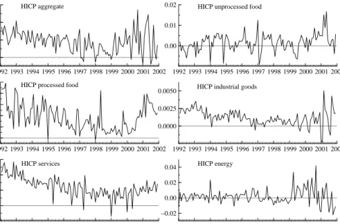
Figure 1:First differences of HICP (sub-)indices (in logarithm)

The month-on-month inflation rates (in decimals) and the year-on-year infla-tion rates (in %) of the indices are displayed in Figures 1 and 2, respectively.

We have carried out Augmented Dickey Fuller (ADF) tests for all HICP (sub-) indices (in logarithms), since Diebold & Kilian (2000) show for univariate models that testing for a unit root can be useful for selecting forecasting models. The tests are based on the sample from 1992(1) to 2000(12). This is the longest of the recursively estimated samples in the simulated out-of-sample forecast experiment (see Section 5.3). The tests do not reject non-stationarity for the levels of all (sub-) indices over the whole period.12Non-stationarity is rejected for the first differences of all series except the aggregate HICP and HICP services. For the first differences of the latter two series, however, non-stationarity is rejected for all shorter recursive

10

Except for interest rates, producer prices and HICP energy that do not exhibit a seasonal pattern. 11

The data used in this study are taken from the ECB and Eurostat. 12

The ADF test specification includes a constant and a linear trend for the levels and first dif-ferences. The number of lags included is chosen according to the largest significant lag on a 5% significance level.

1992 1993 1994 1995 1996 1997 1998 1999 2000 2001 2002 1 2 3 HICP aggregate 1992 1993 1994 1995 1996 1997 1998 1999 2000 2001 2002 0.0 2.5 5.0 7.5

10.0 HICP unprocessed food

1992 1993 1994 1995 1996 1997 1998 1999 2000 2001 2002 1

2 3

4 HICP processed food

1992 1993 1994 1995 1996 1997 1998 1999 2000 2001 2002 1

2

3 HICP industrial goods

1992 1993 1994 1995 1996 1997 1998 1999 2000 2001 2002 2 3 4 5 HICP services 1992 1993 1994 1995 1996 1997 1998 1999 2000 2001 2002 −5 0 5 10 15 HICP energy

estimation samples up to 2000(8) and 2000(7), respectively. Therefore and because of the low power of the ADF test HICP (sub-)indices are assumed to be integrated of order one in the analysis and modeled accordingly.

5.2 Forecast methods and model selection

Different forecasting methods using different model selection procedures are em-ployed for both direct and indirect forecast methods, i.e., forecasting HICP inflation directly versus aggregating subcomponent forecasts. We employ simple autore-gressive (AR) models where the lag length is selected by the Schwarz (SIC) and the Akaike (AIC) criterion respectively (see e.g. Inoue & Kilian, 2005). We include a subcomponent vector autoregressive model (VARsubc) to indirectly forecast the aggregate by aggregating subcomponent forecasts. We use a VAR including the ag-gregate and the components, VARagg,sub, to investigate the hypothesis from section 2 that including component information in the aggregate forecast model improves the forecast of the aggregate. We include a VAR where the lags of the aggre-gate and the components are automatically chosen using PcGets, VARagg,sub_Gets (see Hendry & Krolzig, 2003). In a second group of methods, we include additional macroeconomic predictors in the VARs of the aggregate and the components, re-spectively. This group includes two VARs with a set of domestic and international variables, the VARint, where the specification is the same across the aggregate and the components, and the VARint_Gets, where the specification is allowed to vary across components. Finally, a VAR including potentially all variables, i.e., aggregate, components and other macroeconomic predictors, VARIntAggSub_Gets , is considered.13 The lag length of the VAR is selected on the basis of theSIC, theAIC and an F-test.14

5.3 Simulated out-of-sample forecast comparison

5.3.1 The experiment

A simulated out-of-sample forecast experiment is carried out to evaluate the rela-tive forecast accuracy of alternarela-tive methods to forecast aggregate HICP using in-formation on its disaggregate components as opposed to aggregating the forecasts

13

For the forecast accuracy results presented in the tables of this section model selection proce-dures are carried out on the basis of the first recursive estimation sample until 1998(1). However, recursive model selection was carried out for the most relevant models. The results did not suggest a change to our conclusions.

14

It should be noted that due to the large number of parameters in the high-dimensional VARs the maximum lag order was chosen on the basis of a rough rule such that the total number of parameters in the system would not exceed half the sample size.

of HICP subcomponent models or forecasting the aggregate only using aggregate information. One to twelve step ahead forecasts are performed based on different linear time series models estimated on recursive samples. The main criterion for the comparison of the forecasts employed in this study, as in a large part of the literature on forecasting, is the root mean square forecast error (RMSFE).

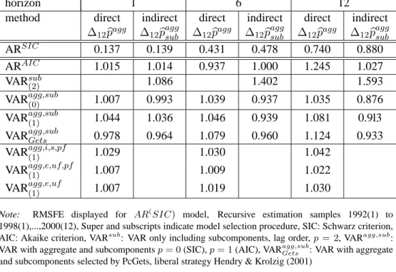
Table 2 and 5 present the comparison of the relative forecast accuracy measured in terms of RMSFE of year-on-year (headline) inflation of the direct forecast of aggregate inflation (∆12bpagg) and the indirect forecast of aggregate inflation, i.e.

the aggregated forecasts of the sub-indices (∆12pbagg_sub). The results for 1-,6- and

12-months ahead forecasts are presented.

5.3.2 Aggregate and disaggregate information

First we compare methods only based on aggregate information as opposed to fore-cast methods for the aggregate including disaggregate variables in addition (see Table 2, column for direct forecast for each forecast horizon). Within the frame-work of the general theory of prediction we have shown that including disaggregate variables in the aggregate model does improve predictability of a variable (see sec-tion 2). We find that the direct forecast using a VAR including the aggregate and subcomponents where the variables are selected by PcGets, VARagg,sub_Gets , performs slightly better inRMSFE terms 1 month ahead than directly forecasting the ag-gregate with an AR model only including lagged agag-gregate information with the

lag length determined by the SIC criterion. Thus, our RMSFE results for the

VARagg,sub_Gets forh = 1confirm this predictability result in a forecast experiment. However, the model including the aggregate and all subcomponents, VARagg,sub₍₁₎ does not provide a more accurate forecast of the aggregate than the autoregressive models ARSICand ARAIC.

Furthermore, we investigate the accuracy of forecasting the aggregate directly including disaggregate variables relative to the forecast accuracy of indirectly fore-casting the aggregate by aggregating component forecasts based on an AR model or a subcomponent VAR,V ARsub, (Table 2), i.e., the way previous literature has been taken disaggregate variables into account (see e.g. Hubrich (2004)). The VAR model that outperforms the other direct forecast methods of the aggregate, VARagg,sub_Gets , also exhibits higher forecast accuracy for the indirect forecast than all other methods forh = 1. Thus, including aggregate variables in the disaggregate model improves forecast performance for short horizons. The VARagg,sub_Gets does also outperform the VARagg,sub₍₁₎ , where the variables and lag length are the same across the aggregate and components, forh= 1.

Overall, the direct forecast including the aggregate and subcomponents is best for 1 month ahead forecasts if no additional macroeconomic indicators are

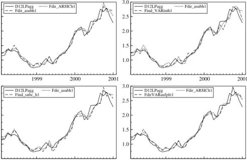
con-1999 2000 2001 1.0 1.5 2.0 2.5 3.0 D12LPagg Fdir_asubh1 Fdir_ARSICh1 1999 2000 2001 1.0 1.5 2.0 2.5 3.0 D12LPagg Find_VARinth1 Fdir_asubh1 1999 2000 2001 1.0 1.5 2.0 2.5 3.0 D12LPagg Find_subc_h1 Fdir_asubh1 1999 2000 2001 1.0 1.5 2.0 2.5 3.0 D12LPagg FdirVARaufpfe1 Fdir_ARSICh1

Figure 3:Year-on-year inflation rate and forecasts in %, 1 months ahead, solid line: actual, Fdir: direct forecast of aggregate, Find: indirect forecast of aggregate

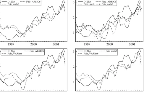
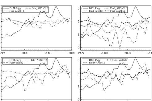
sidered. That confirms within a forecasting set-up the results derived with respect to predictability in section 2, i.e. that forecasting the aggregate directly including disaggregate information in the aggregate model might perform better than aggre-gating component forecasts. Figure 3 shows that the one months ahead forecasts from the different methods are very close to actual year-on-year inflation. The dif-ferences between the different methods for one month ahead forecasts appear to be quite small. Figure 4 presents the forecast 6 months ahead. Six months ahead forecasts of year-on-year inflation do generally relatively well. The graphs show that the differences in RMSFE terms between some of the forecasts are relevant to be considered when choosing the forecasting model.

1999 2000 2001 1 2 3 D12Lp Fdir_asub6 Fdir_ARSIC6 1999 2000 2001 1 2 3 D12Lp

Find_sub6 Find_ARSIC6 Fdir_asub6

1999 2000 2001 1 2 3 D12Lp Fdir_VARint6 Fdir_ARSIC6 1999 2000 2001 1 2 3 D12Lp Fdir_VARint6 Fdir_asub6

Figure 4:Year-on-year inflation rate and forecasts in %, 6 months ahead, solid line: actual, Fdir: direct forecast of aggregate, Find: indirect forecast of aggregate

More important from a monetary policy point of view is the 12 months ahead forecast. Here we find that the direct forecast including disaggregate information (VARagg,sub₍₁₎ ) is clearly better than the indirect forecast based on AR or VAR mod-els of the components. The low forecast accuracy of aggregating subcomponent models is analyzed in Hubrich (2004), and it is found that this is due to unexpected shocks that occur in the forecast period and affect some or all components in the same direction so that forecast errors do not cancel. Furthermore, predictability