Forecasting with Spatial Panel Data

DISCUSSION PAPER SERIES

Forschungsinstitut

zur Zukunft der Arbeit

Institute for the Study

Forecasting with Spatial Panel Data

IZA DP No. 4242

June 2009

Badi H. Baltagi

Georges Bresson

Alain Pirotte

Forecasting with Spatial Panel Data

Badi H. Baltagi

Syracuse University

and IZA

Georges Bresson

ERMES (CNRS), Université Panthéon-Assas Paris II

Alain Pirotte

ERMES (CNRS), Université Panthéon-Assas Paris II

and INRETS-DEST

Discussion Paper No. 4242

June 2009

IZA

P.O. Box 7240

53072 Bonn

Germany

Phone: +49-228-3894-0

Fax: +49-228-3894-180

E-mail: [email protected]

Any

opinions expressed here are those of the author(s) and not those of IZA. Research published in

this series may include views on policy, but the institute itself takes no institutional policy positions.

The Institute for the Study of Labor (IZA) in Bonn is a local and virtual international research center

and a place of communication between science, politics and business. IZA is an independent nonprofit

organization supported by Deutsche Post Foundation. The center is associated with the University of

Bonn and offers a stimulating research environment through its international network, workshops and

conferences, data service, project support, research visits and doctoral program. IZA engages in (i)

original and internationally competitive research in all fields of labor economics, (ii) development of

policy concepts, and (iii) dissemination of research results and concepts to the interested public.

IZA Discussion Papers often represent preliminary work and are circulated to encourage discussion.

IZA Discussion Paper No. 4242

June 2009

ABSTRACT

Forecasting with Spatial Panel Data

*

This paper compares various forecasts using panel data with spatial error correlation. The

true data generating process is assumed to be a simple error component regression model

with spatial remainder disturbances of the autoregressive or moving average type. The best

linear unbiased predictor is compared with other forecasts ignoring spatial correlation, or

ignoring heterogeneity due to the individual effects, using Monte Carlo experiments. In

addition, we check the performance of these forecasts under misspecification of the spatial

error process, various spatial weight matrices, and heterogeneous rather than homogeneous

panel data models.

JEL Classification:

C33

Keywords:

forecasting, BLUP, panel data, spatial dependence, heterogeneity

Corresponding author:

Badi H. Baltagi

Department of Economics and Center for Policy Research

426 Eggers Hall

Syracuse University

Syracuse, NY 13244-1020

USA

E-mail:

[email protected]

*

This paper was presented at a conference in honor of Phoebus Dhrymes in Paphos, Cyprus, June

1-3, 2007. Also, at the 14th International Conference on Panel Data at the Wang Yanan Institute for

Studies in Economics (WISE), Xiamen University, China, July 16-18, 2007, and the 63rd European

1

Introduction

The literature on forecasting is rich with time series applications, but this

is not the case for spatial panel data applications. Exceptions are Baltagi

and Li (2004, 2006) with applications to forecasting sales of cigarettes and

liquor per capita for U.S. states over time.

1

_{Best linear unbiased prediction}

(BLUP) in panel data using an error component model have been

consid-ered by Taub (

1

979), Baltagi and Li (

1

992), and Baillie and Baltagi (

1

999)

to mention a few. Applications include Baltagi and Gri

ffi

n (

1

997), Hsiao

and Tahmiscioglu (

1

997), Schmalensee, Stoker and Judson (

1

998), Baltagi,

Gri

ffi

n and Xiong (2000), Hoogstrate, Palm and Pfann (2000), Baltagi,

Bres-son and Pirotte (2002, 2004), Frees and Miller (2004), Rapach and Wohar

(2004), and Brucker and Siliverstovs (2006), see Baltagi (2008) for a recent

survey. However, these panel forecasting applications do not deal with spatial

dependence across the panel units. Spatial dependence models – popular

in regional science and urban economics – deal with spatial interaction and

spatial heterogeneity (see Anselin (

1

988) and Anselin and Bera (

1

998)). The

structure of the dependence can be related to location and distance, both in a

geographic space as well as a more general economic or social network space.

Some commonly used spatial error processes include the spatial

autoregres-sive (SAR) and the spatial moving average (SMA) error processes. Two

di

ff

erent variants of these models for spatial panels are considered, one

dis-cussed in Anselin (

1

988) and another in Kapoor, Kelejian and Prucha (2007)

and Fingleton (2007). The best linear unbiased predictors for the Anselin

type model was derived by Baltagi and Li (2004). This paper derives the best

linear unbiased predictors for the Kapoor, Kelejian and Prucha (2007) and

Fingleton (2007) variants. More importantly, it compares the performance of

sixteen various forecasts of the spatial panel data using Monte Carlo

exper-iments. These include homogeneous as well as heterogeneous estimators of

the spatial panel model and their corresponding forecasts. The true data

gen-erating process is assumed to be a simple error component regression model

with spatial remainder disturbances of the autoregressive or moving average

1

_{In order to explain how spatial autocorrelation may arise in the demand for cigarettes,}

we note that cigarette prices vary among states primarily due to variation in state taxes

on cigarettes. Border e

ff

ect purchases not included in the cigarette demand equation can

cause spatial autocorrelation among the disturbances. In forecasting sales of cigarettes, the

spatial autocorrelation due to neighboring states and the individual heterogeneity across

states is taken explicitly into account.

type. The best linear unbiased predictor is compared with other forecasts

ignoring spatial correlation, or ignoring heterogeneity due to the individual

e

ff

ects. In addition, we check the performance of these forecasts under

mis-speci

fi

cation of the spatial error process, di

ff

erent spatial weight matrices,

and various sample sizes. Section 2 introduces the error component model

with spatially autocorrelated residuals of the SAR and SMA type. Section

3 describes the forecasts using the estimators considered in Section 2, while

Section 4 gives the Monte Carlo design. Section 5 reports the results of the

Monte Carlo simulations and Section 6 gives our summary and conclusion.

2

The Error Component Model with Spatially

Autocorrelated Residuals

Consider a linear panel data regression model:

y

it

=

X

it

β

+

ε

it

,

i

= 1

, ..., N

;

t

= 1

, ..., T

(

1

)

where the disturbance term follows an error component model with spatially

autocorrelated residuals. The disturbance vector for time

t

is given by:

ε

t

=

µ

+

φ

t

(2)

where

ε

t

= (

ε

1t

, ...,

ε

N t)0

,

µ

= (

µ

1

, ..., µ

N

)

0

denotes the vector of speci

fi

c

ef-fects assumed to be

iid

¡

0

,

σ

2

µ

¢

and

φ

_t

= (

φ

_1t

, ...,

φ

_{N t}

)

0

are the remainder

disturbances which are independent of

µ

. We let the

φ

t

’s follow a spatial

autoregressive (SAR) or a spatial moving average (SMA) error model. The

SAR process is known to transmit the shocks globally while the SMA process

transmits these shocks locally, see Anselin, Le Gallo and Jayet (2008).

The SAR speci

fi

cation for the

(

N

_×

1)

error vector

φ

_t

at time

t

can be

ex-pressed as:

φ

t

=

ρ

W

N

φ

t

+

v

t

= (

I

N

−

ρ

W

N

)

−

1

v

t

=

B

N−1

v

t

(3)

where

W

N

is an

(

N

×

N

)

known spatial weights matrix

2

,

ρ

is the spatial

au-toregressive parameter and

v

t

is an

(

N

×

1)

error vector assumed to be

dis-2

_{In the simplest case, the weights matrix is binary, with}

_w

ij

= 1

when

i

and

j

are

neighbors and

w

ij

= 0

when they are not. By convention, diagonal elements are null:

wii

= 0

and the weights are almost always standardized such that the elements of each

row sum to

1

.

tributed independently across cross-sectional dimension with constant

vari-ance

σ

2v

I

N

.

B

N

= (

I

N

−

ρ

W

N

)

and is assumed to be non-singular. The error

covariance matrix for the cross-section at time

t

becomes:

Ω

t

=

E

[

ε

t

ε

0t

] =

σ

2

µ

I

N

+

σ

2v

(

B

N0

B

N

)

−

1

(4)

For the full

(

N T

_×

1)

vector of disturbances:

ε

= (

ι

T

⊗

I

N

)

µ

+

¡

I

T

⊗

B

N−1

¢

v

(5)

the corresponding

(

N T

_×

N T

)

covariance matrix is given by:

Ω

=

σ

2_µ

(

J

T

⊗

I

N

) +

σ

2v

h

I

T

⊗

(

B

N0

B

N

)

−

1

i

(6)

where

ι

T

is a

(

T

×

1)

vector of ones and

J

T

=

ι

T

ι

0T

is a

(

T

×

T

)

matrix of

ones.

The spatial moving average (SMA) speci

fi

cation for the

(

N

_×

1)

error vector

φ

t

at time

t

can be expressed as:

φ

_t

=

λ

W

N

v

t

+

v

t

= (

I

N

+

λ

W

N

)

v

t

=

D

N

v

t

(7)

where

D

N

= (

I

N

+

λ

W

N

)

.

The error covariance matrix for the cross-section

at time

t

becomes:

Ω

t

=

E

[

ε

t

ε

0t

] =

σ

2

µ

I

N

+

σ

2v

(

D

N

D

0N

)

(8)

For the full

(

N T

_×

1)

vector of disturbances:

ε

= (

ι

T

⊗

I

N

)

µ

+ (

I

T

⊗

D

N

)

v

(9)

the corresponding

(

N T

_×

N T

)

covariance matrix is given by:

Ω

=

σ

2µ

(

J

T

⊗

I

N

) +

σ

v2

[

I

T

⊗

(

D

N

D

0N

)]

(

1

0)

MLE under normality of the disturbances using these error component

mod-els with spatial autocorrelation have been derived by Anselin (

1

988). The

log-likelihood is given by:

L

∝

₋

N T

2

ln

¡

2

πσ

2_v

¢

₋

1

2

ln

|

Σ

|

−

1

2

σ

2 v

ε

0

Σ

−1

ε

(

11

)

where

ε

=

y

₋

X

β

,

Ω

=

σ

2v

Σ

Σ

=

½

(

J

T

⊗

θ

I

N

) +

£

I

T

⊗

(

B

N0

B

N

)

− 1

¤

for SAR

(

J

T

⊗

θ

I

N

) + [

I

T

⊗

(

D

N

D

N0

)]

for SMA

(

1

2)

with

θ

=

σ

2µ

/

σ

2v

.

Regression models containing spatially correlated disturbance terms based

on the SAR or SMA models are typically estimated using MLE, where the

likelihood function corresponds to the normal distribution. However, this can

be computationally demanding for large

N

. Kelejian and Prucha (

1

999)

sug-gested a generalized moments (GM) estimation method for the SAR model

in a cross-section setting, and Fingleton (2007) extended this generalized

moments estimator to the SMA model. Kapoor, Kelejian and Prucha (2007)

generalized this GM procedure from cross-section to panel data and derived

its large sample properties when

T

is

fi

xed and

N

_{→ ∞}

. However, their SAR

random e

ff

ects model (SAR-RE) di

ff

ers from that described in (2) which we

will call (RE-SAR). In fact, in their speci

fi

cation, the disturbance term

ε

t

itself follows a SAR process and the remainder term follows an error

compo-nent structure. This allows the individual e

ff

ects, i.e., the

µ

’s themselves to

be spatially correlated but with the same

ρ

. In particular, the disturbance

vector for time

t

is given by:

ε

t

=

ρ

W

N

ε

t

+

u

t

(

1

3)

where

u

t

follows an error component structure :

u

t

=

µ

+

v

t

(

1

4)

The SAR-RE speci

fi

cation for the

(

N

_×

1)

error vector

ε

t

at time

t

can be

expressed as:

ε

t

= (

I

N

−

ρ

W

N

)

−

1

u

t

=

B

N−1

u

t

(

1

5)

where

B

N

= (

I

N

−

ρ

W

N

)

.

For the full

(

N T

×

1)

vector of disturbances:

ε

=

¡

ι

T

⊗

B

N−1

¢

µ

+

¡

I

T

⊗

B

N−1

¢

v

(

1

6)

and the corresponding

(

N T

_×

N T

)

covariance matrix is given by:

Ω

=

σ

2_µ

³

J

T

⊗

(

B

N0

B

N

)

−

1

´

+

σ

2_v

h

I

T

⊗

(

B

0N

B

N

)

−

1

i

Kapoor, et al. (2007) proposed three generalized moments (GM) estimators

of

ρ

,

σ

2v

and

σ

21

¡

=

σ

2v

+

T

σ

2µ

¢

based on the following six moment conditions:

E



















1 N(T−1)

u

0 N

Q

0,N

u

N 1 N(T−1)

u

0 N

Q

0,N

u

N 1 N(T−1)

u

0 N

Q

0,N

u

N 1 N

u

0 N

Q

1,N

u

N 1 N

u

0 N

Q

1,N

u

N 1 N

u

0 N

Q

1,N

u

N



















=

















σ

2 v

σ

2 v 1 N

tr

¡

W

_N0

W

N

¢

0

σ

21

σ

2 1N1

tr

¡

W

_N0

W

N

¢

0

















(

1

8)

where

u

N

=

ε

N

−

ρε

N

(

1

9)

u

N

=

ε

N

−

ρε

N

(20)

ε

N

= (

I

T

⊗

W

N

)

ε

N

(2

1

)

ε

N

= (

I

T

⊗

W

N

)

ε

N

(22)

Q

0,N

=

µ

I

T

−

J

T

T

¶

⊗

I

N

(23)

Q

1,N

=

J

T

T

⊗

I

N

(24)

Under the random e

ff

ects speci

fi

cation considered, the OLS estimator of

β

is

consistent. Using

b

β

OLS

one gets a consistent estimator of the disturbances

b

ε

=

y

₋

X

β

b

_OLS

.

The GM estimators of

σ

2

1

,

σ

2ν

and

ρ

are the solution of

the sample counterpart of the six equations given above. Kapoor, et al.

(2007) suggest three GM estimators. The

fi

rst involves only the

fi

rst three

moments which do not involve

σ

2

1

and yield estimates of

ρ

and

σ

2ν

. The fourth

moment condition is then used to solve for

σ

2

1

given estimates of

ρ

and

σ

2ν

. The

second GM estimator is based upon weighing the moment equations by the

inverse of a properly normalized variance-covariance matrix of the sample

moments evaluated at the true parameter values. A simple version of this

weighting matrix is derived under normality of the disturbances. The third

GM estimator is motivated by computational considerations and replaces

a component of the weighting matrix for the second GM estimator by an

identity matrix. Kapoor, et al. (2007) perform Monte Carlo experiments

comparing MLE and these three GM estimation methods. They

fi

nd that

similar. The feasible GLS estimator of

β

is then obtained by replacing

ρ

,

σ

2

v

and

σ

21

by their GM estimators.

3

Recently, Fingleton (2007) extended this GM estimator for the SMA panel

data model with random e

ff

ects. We call this SMA-RE to distinguish it

from the RE-SMA procedure described in Anselin, et al. (2008). In fact,

for the Fingleton (2007) SMA-RE, the disturbance term

ε

t

in (2) follows a

SMA process and the remainder term follows an error component structure.

Unlike the Anselin, et al. (2008) RE-SMA, the individual e

ff

ects, i.e., the

µ

’s themselves are allowed to be spatially correlated but with the same

λ

. In

particular, the disturbance vector for time

t

is given by:

ε

t

= (

I

N

+

λ

W

N

)

u

t

=

D

N

u

t

(25)

where

D

N

= (

I

N

+

λ

W

N

)

, and

u

t

follows an error component structure (

1

4).

So, the full SMA-RE

(

N T

_×

1)

vector of disturbances is given by:

ε

= (

ι

T

⊗

D

N

)

µ

+ (

I

T

⊗

D

N

)

v

(26)

and the corresponding

(

N T

_×

N T

)

covariance matrix is given by:

Ω

=

σ

2_µ

(

J

T

⊗

(

D

N

D

0N

)) +

σ

2

v

[

I

T

⊗

(

D

N

D

0N

)]

(27)

The moment conditions for SMA-RE are similar to those derived by Kapoor,

et al. (2007), see Fingleton (2007).

3

Prediction

Goldberger (

1

962) has shown that, for a given

Ω

, the best linear unbiased

predictor (BLUP) for the

i

th individual at a future period

T

+

τ

is given by:

b

y

i,T+τ

=

X

i,T+τ

b

β

GLS

+

ω

0

Ω

−

1

b

ε

GLS

(28)

where

ω

=

E

[

ε

i,T+τ

ε

]

is the covariance between the future disturbance

ε

i,T+τ

and the sample disturbances

ε

.

β

b

_GLS

is the GLS estimator of

β

from equation

(

1

) based on

Ω

and

_b

ε

GLS

denotes the corresponding GLS residual vector.

3

_{Later, in our Monte Carlo experiments, we computed the predictors for all three GM}

estimators suggested by Kapoor, et al. (2007). However, the di

ff

erences in root mean

squared error performance were minor. To save space, we only report the second GM

estimator, called weighted GM estimator by Kapoor, et al. (2007).

For the error component without spatial autocorrelation (

λ

= 0

), this BLUP

reduces to:

b

y

i,T+τ

=

X

i,T+τ

β

b

GLS

+

σ

2 µ

σ

2 1

(

ι

0_T

_⊗

l

_i0

)

_b

ε

GLS

(29)

where

σ

2

1

=

T

σ

2µ

+

σ

v2

and

l

i

is the

i

th column of

I

N

. This predictor was

considered by Wansbeek and Kapteyn (

1

978), Lee and Gri

ffi

ths (

1

979) and

Taub (

1

979).

The typical element of the last term of equation (29) is

¡

T

σ

2

µ

/

σ

21

¢

ε

i.,GLS

where

ε

i.,GLS

=

P

T_t=1

b

ε

ti,GLS

/T

. Therefore, the BLUP of

y

i,T+τ

for the RE model modi

fi

es the usual GLS forecasts by adding a

frac-tion of the mean of the GLS residuals corresponding to the

i

th individual.

In order to make this forecast operational,

b

β

_GLS

is replaced by its feasible

GLS estimate and the variance components are replaced by their feasible

estimates.

Baltagi and Li (2004, 2006) derived the BLUP correction term when

both error components and spatial autocorrelation are present and

φ

t

follows

a SAR process. So, the predictors for the SAR and the SMA are given by:

b

y

i,T+τ

=



































X

i,T+τ

β

b

M LE

+

θ

¡

ι

0 T

⊗

l

0i

C

− 1 1

¢

b

ε

M LE

=

X

i,T+τ

β

b

M LE

+

T

θ

N

P

j=1

c

1,j

ε

j.,M LE

for SAR

X

i,T+τ

β

b

M LE

+

θ

¡

ι

0T

⊗

l

0i

C

2−1

¢

b

ε

M LE

=

X

i,T+τ

β

b

M LE

+

T

θ

N

P

j=1

c

2,j

ε

j.,M LE

for SMA

(30)

where

c

1j

(resp.

c

2,j

) is the

j

th element of the

i

th row of

C

1−1

(resp.

C

2−1

) with

C

1

=

£

T

θ

I

N

+ (

B

N0

B

N

)

−1

¤

(resp.

C

2

= [

T

θ

I

N

+ (

D

N

D

0N

)]

) and

ε

j.,M LE

=

P

T

t=1

b

ε

tj,M LE

/T

. In other words, the BLUP of

y

i,T+τ

adds to

X

i,T+τ

β

b

M LE

a weighted average of the MLE residuals for the

N

individuals averaged

over time. The weights depend upon the spatial matrix

W

N

and the

spa-tial autoregressive (or moving average) coe

ffi

cients

ρ

and

λ

. To make these

predictors operational, we replace

θ

,

ρ

and

λ

by their estimates from the

RE-spatial MLE with SAR or SMA. When there are no random individual

e

ff

ects, so that

σ

2

µ

= 0

,

then

θ

= 0

and the BLUP prediction terms drop out

completely from equation (30). In these cases,

Ω

in equation (

1

2) reduces to

σ

2

v

£

I

T

⊗

(

B

N0

B

N

)

−1

¤

for SAR and

σ

2

v

[

I

T

⊗

(

D

N

D

N0

)]

for SMA, and the

cor-responding MLE for these models yield the pooled spatial MLE with SAR

or SMA remainder disturbances.

For the Kapoor, et al. (2007) model, the BLUP of

y

i,T+τ

for the SAR-RE

also modi

fi

es the usual GLS forecasts by adding a fraction of the mean of

the GLS residuals corresponding to the

i

th individual. More speci

fi

cally, the

predictor is given by:

b

y

i,T+τ

=

X

i,T+τ

b

β

GLS

+

µ

_σ

2 µ

σ

2 1

¶

b

i

(

ι

0T

⊗

B

N

)

b

ε

GLS

(3

1

)

where

b

i

is the

i

th row of the matrix

B

N−1

. This is derived in the Appendix

of this paper which also shows the resulting predictor has the same form as

that of the RE model (29). This proof applies to both the Kapoor, et al.

(2007) SAR-RE speci

fi

cation and the Fingleton (2007) SMA-RE speci

fi

ca-tion. Therefore, the BLUP of

y

i,T+τ

for the SAR-RE and the SMA-RE, like

the usual RE model with no spatial e

ff

ects, modi

fi

es the usual GLS forecasts

by adding a fraction of the mean of the GLS residuals corresponding to the

i

th individual. While the predictor formula is the same, the MLEs for these

speci

fi

cations yield di

ff

erent estimates which in turn yield di

ff

erent residuals

and hence di

ff

erent forecasts.

4

Monte Carlo Design

In this section, we consider the small sample performance of several predictors

for an error component model with spatially autocorrelated residuals. The

data generating process (DGP) consider two speci

fi

cations on the remainder

errors, namely SAR and SMA:

y

it

=

β

0

+

β

1

x

it

+

ε

it

,

ε

it

=

µ

i

+

φ

it

,

i

= 1

, ..., N

;

t

= 1

, ..., T

(32)

where

4

x

it

=

δ

i

+

ξ

it

with

µ

i

∼

iid.N

¡

0

,

σ

2_µ

¢

,

δ

i

∼

iid.U

(

−

7

.

5

,

7

.

5)

,

ξ

_it

_∼

iid.U

(

₋

5

,

5)

,

β

₀

= 5

,

β

₁

= 0

.

5

4

_{In the spirit of Nerlove (}

₁

₉₇

₁

_{), we have tried another DGP for}

_xit

_{. We obtain the}

same ranking as those which appear in the reported tables. The only di

ff

erence is that

the gap between the average heterogeneous estimators and the homogeneous estimators

widens with a Nerlove (

1

97

1

) type design. In other words, the forecast performance of the

heterogeneous estimators becomes worse.

φ

_t

=

½

ρ

W

N

φ

t

+

v

t

for SAR

λ

W

N

v

t

+

v

t

for SMA

with

ρ

,

λ

=

½

0

.

8

0

.

4

(33)

and

v

it

∼

iid.N

¡

0

,

σ

2v

¢

(34)

We consider the simple regressions (32) and (33) with

N

= (50

,

100)

,

T

=

(10

,

20)

and two cases for the residuals variances:

½

σ

2µ

= 4

,

σ

2v

= 16

σ

2µ

= 16

,

σ

2v

= 4

(35)

Following Kelejian and Prucha (

1

999), we use two weight matrices which

es-sentially di

ff

er in their degree of sparseness. The weight matrices are labelled

as “

j

ahead and

j

behind” with the non-zero elements being

1

/

2

j

,

j

= 1

and

5

. Even with this modest design we have 64 experiments.

For each experiment, we obtain the following

1

6 estimators:

1

. Pooled OLS which ignores the individual heterogeneity and the spatial

autocorrelation.

2. The average heterogeneous OLS which estimates the cross-sectional

equation using OLS for each time period and averages these

heteroge-neous estimates to obtain a pooled estimator, see Pesaran and Smith

(

1

995).

3. The

fi

xed-e

ff

ects (FE) estimator which accounts for

fi

xed individual

e

ff

ects but does not take into account the spatial autocorrelation.

4. The random e

ff

ects (RE) estimator which asssumes that the

µ

i

’s are

iid

(0

,

σ

2

µ

)

,

and independent of the remainder disturbances

φ

it

’s. This

estimator accounts for random individual e

ff

ects but does not take into

account the spatial autocorrelation.

5. The RE-spatial MLE assuming a SAR speci

fi

cation (RE-SAR) on the

remainder disturbances. In this case, the

µ

_i

’s are

iid

(0

,

σ

2

µ

)

and are

independent of the

φ

it

’s which follow a SAR process, see Anselin, et al.

6. The RE-spatial MLE assuming a SMA speci

fi

cation (RE-SMA) on the

remainder disturbances. In this case, the

µ

i

’s are

iid

(0

,

σ

2µ

)

and are

independent of the

φ

_it

’s which follow a SMA process, see Anselin, et

al. (2008).

7. The pooled spatial MLE assuming a SAR speci

fi

cation (Pooled SAR)

on the remainder disturbances. This estimator ignores the individual

heterogeneity but takes into account the spatial autocorrelation of the

SAR type.

8. The pooled spatial MLE assuming a SMA speci

fi

cation (Pooled SMA)

on the remainder disturbances. This estimator ignores the individual

heterogeneity but takes into account the spatial autocorrelation of the

SMA type.

9. The average heterogeneous spatial MLE assuming a SAR speci

fi

cation

on the remainder disturbances. This estimates cross-sectional MLE

with SAR disturbances for each time period and averages the estimates

over time.

1

0. The average heterogeneous spatial GM estimator assuming a SAR

speci

fi

cation on the remainder disturbances proposed by Kelejian and

Prucha (

1

999). This estimates cross-sectional GM estimator with SAR

disturbances for each time period and averages the estimates over time.

11

. The average heterogeneous spatial MLE assuming a SMA speci

fi

cation

on the remainder disturbances. This estimates cross-sectional MLE

with SMA disturbances for each time period and averages the estimates

over time.

1

2. The average heterogeneous spatial GM estimator assuming a SMA

speci

fi

cation on the remainder disturbances proposed by Fingleton (2007).

This estimates cross-sectional GM estimator with SMA disturbances for

each time period and averages the estimates over time.

1

3. The FE-spatial MLE assuming a SAR speci

fi

cation (FE-SAR) on the

remainder disturbances.

1

4. The FE-spatial MLE assuming a SMA speci

fi

cation (FE-SMA) on the

1

5. The (SAR-RE) model following Kapoor, et al. (2007). This utilizes

a panel data GM estimator where the disturbance term itself follows

a SAR process and the remainder term follows an error component

structure.

1

6. The (SMA-RE) model following Fingleton (2007). This utilizes a panel

data GM estimator where the disturbance term itself follows a SMA

process and the remainder term follows an error component structure.

Next, we compute the following predictors for the

i

th individual at a

fu-ture period

T

+

τ

for

τ

= 1

,

2

, ...,

5

:

OLS

y

_b

i,T+τ

=

X

i,T+τ

β

b

OLS

Average hetero. OLS

y

_b

i,T+τ

=

X

i,T+τ

β

b

av.OLS

FE

5

(

b

y

i,T+τ

=

X

i,T+τ

b

β

F E

+

b

µ

i

with

µ

_b

_i

=

y

_i

₋

X

i

b

β

F E

,

y

i

=

P

T t=1

y

it

/T

RE

y

_b

i,T+τ

=

X

i,T+τ

β

b

RE

+

σ2 µ σ2 1

(

ι

0 T

⊗

l

0i

)

b

ε

RE

RE-SAR

½

b

y

i,T+τ

=

X

i,T+τ

b

β

M LE,RE−SAR

+

θ

¡

ι

0 T

⊗

l

0i

C

− 1 1

¢

b

ε

M LE,RE−SAR

with

C

1

=

£

T

θ

I

N

+ (

B

N0

B

N

)

−1

¤

and

θ

=

σ

2µ

/

σ

2v

RE-SMA

½

b

y

i,T+τ

=

X

i,T+τ

b

β

M LE,RE−SM A

+

θ

¡

ι

0 T

⊗

l

i0

C

− 1 2

¢

b

ε

M LE,RE−SM A

with

C

2

= [

T

θ

I

N

+ (

D

N

D

0N

)]

and

θ

=

σ

2µ

/

σ

2v

Pooled SAR

y

_b

i,T+τ

=

X

i,T+τ

β

b

M LE,SAR

Pooled SMA

y

_b

i,T+τ

=

X

i,T+τ

β

b

M LE,SM A

Average hetero. SAR

b

y

i,T+τ

=

(

X

i,T+τ

b

β

av.M LE,SAR

X

i,T+τ

b

β

av.GM,SAR

Average hetero. SMA

_b

y

i,T+τ

=

(

X

i,T+τ

b

β

av.M LE,SM A

X

i,T+τ

b

β

av.GM,SM A

FE-SAR

(

b

y

i,T+τ

=

X

i,T+τ

b

β

M LE,F E−SAR

+

b

µ

i

with

µ

_b

i

=

y

i

−

X

i

b

β

M LE,F E−SAR

,

y

i

=

P

T

t=1

y

it

/T

FE-SMA

(

b

y

i,T+τ

=

X

i,T+τ

b

β

M LE,F E−SM A

+

µ

b

i

with

µ

b

i

=

y

i

−

X

i

b

β

M LE,F E−SM A

,

y

i

=

P

T

t=1

y

it

/T

SAR-RE

_b

y

i,T+τ

=

X

i,T+τ

b

β

M LE,SAR−RE

+

³

_σ2 µ σ2 1

´

(

ι

0 T

⊗

l

0i

)

b

ε

M LE,SAR−RE

SMA-RE

_b

y

i,T+τ

=

X

i,T+τ

b

β

M LE,SM A−RE

+

³

_σ2 µ σ2 1

´

(

ι

0 T

⊗

l

0i

)

b

ε

M LE,SM A−RE

For all experiments,

1

000 replications are performed and the RMSE for

one step to

fi

ve step ahead forecasts are reported.

5

Monte Carlo Results

5.1

The Spatial Dependence Speci

fi

cation E

ff

ect

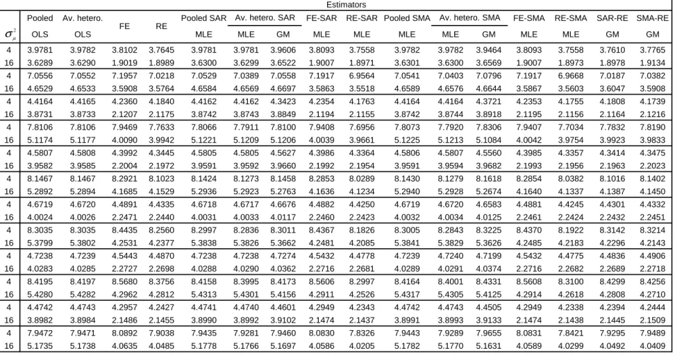
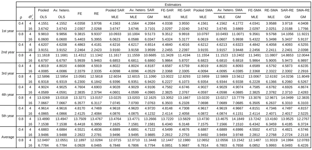
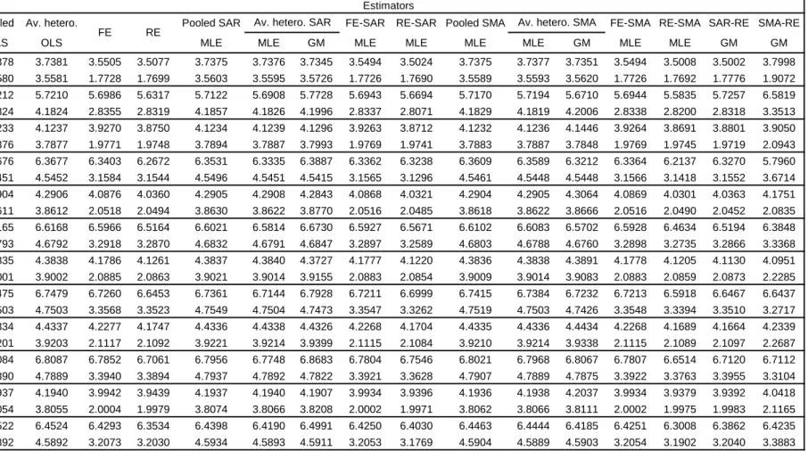
Table

1

gives the RMSE for the one year, two year,..., and

fi

ve year ahead

forecasts along with the average RMSE for all 5 years. These are out of

sam-ple forecasts when the true DGP is a RE panel model with SAR remainder

disturbances. The sample size is

N

= 50

and

T

= 10

,

the weight matrix is

W(

1

,

1

), i.e., one neighbor behind and one neighbor ahead. In general, for

ρ

= 0

.

4

,

0

.

8

and

σ

2µ

= 4

,

16

,

the lowest RMSE is that of RE-SAR. This is

fol-lowed closely by SAR-RE and SMA-RE. It con

fi

rms the

fi

ndings of Kapoor,

et al. (2007) that, on average, RMSE of MLE and their GM estimators are

quite similar. It also seems like misspecifying the SAR by an SMA in an error

component model does not a

ff

ect the forecast performance as long as it is

taken into account. As the spatial autoregressive parameter

ρ

doubles from

0

.

4

to

0

.

8

, the RMSE also doubles. The RMSE improves as

σ

2

µ

gets large,

i.e.,

16

rather than

4

,

for estimators that take heterogeneity into account.

Pooled OLS, average heterogeneous OLS, pooled SAR, pooled SMA, average

heterogeneous SAR (MLE and GM) and average heterogeneous SMA (MLE

and GM) perform worse in terms of RMSE than spatial/panel homogeneous

estimators. This forecast comparison is robust whether we are predicting

one period, two periods or 5 periods ahead and is also re

fl

ected in the

av-erage over the

fi

ve years. The gain in forecast performance is substantial

once we account for RE or FE and is only slightly improved by additionally

accounting for spatial autocorrelation, i.e., FE-SAR or RE-SAR, FE-SMA,

or RE-SMA.

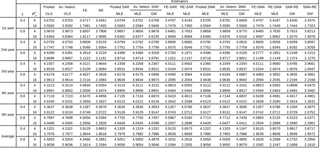
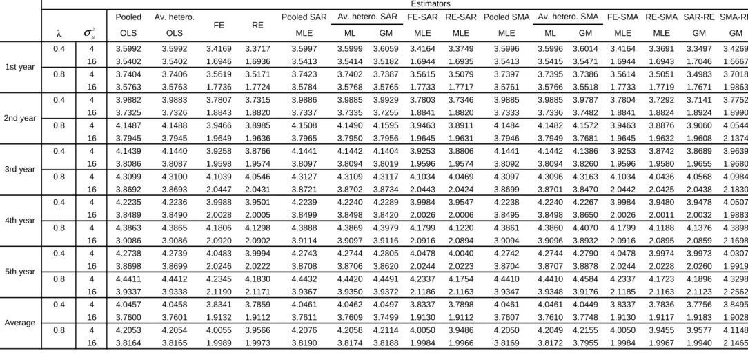
Table 2 gives the RMSE results when the true DGP is a RE panel model

with SMA remainder disturbances. The sample size is still

N

= 50

, T

= 10

,

and the weight matrix is W(

1

,

1

). In general, for

ρ

= 0

.

4

,

0

.

8

and

σ

2

µ

= 4

,

16

,

the lowest RMSE is that of RE-SMA. This is followed closely by RE-SAR.

5

_{See Baillie and Baltagi (}

₁

_998).

Misspecifying the SMA by an SAR in an error component model does not

seem to a

ff

ect the forecast performance as long as it is taken into account.

However, the magnitudes of the RMSE in Table 2 (where the true DGP is

a RE-SMA process) are much lower than those in Table

1

(where the true

DGP is a RE-SAR process). Once again, the forecast RMSE of based on

MLE and their GM counterparts are quite similar, compare SAR-RE and

SMA-RE with RE-SAR and RE-SMA. The RMSE improves as

σ

2

µ

gets large,

i.e.,

16

rather than

4

,

for estimators that take heterogeneity into account. As

the spatial autoregressive parameter

λ

increases from

0

.

4

to

0

.

8

, the RMSE

also increases but not as much as it did for the SAR process in Table

1

.

Pooled OLS, average heterogeneous OLS, pooled SAR, pooled SMA, average

heterogeneous SAR (MLE and GM) and average heterogeneous SMA (MLE

and GM) perform worse in terms of RMSE than spatial/panel homogeneous

estimators. This forecast performance is robust whether we are predicting

one period, two periods or 5 periods ahead and is also re

fl

ected in the average

over the

fi

ve years. Once again, the gain in forecast performance is substantial

once we account for RE or FE and is only slightly improved by additionally

accounting for spatial autocorrelation, i.e., FE-SMA, or RE-SMA, FE-SAR

or RE-SAR.

5.2

Sensitivity Analysis

5.2.1

The Spatial Weight Matrix e

ff

ect

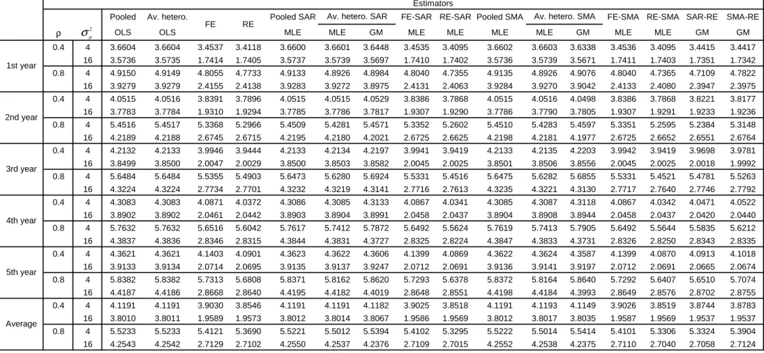
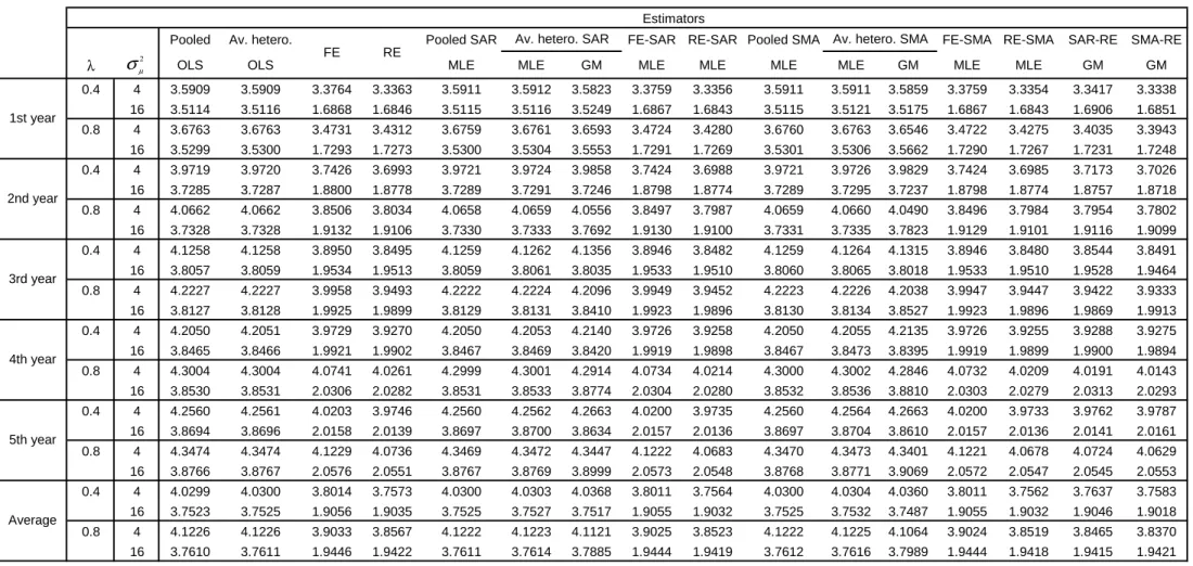
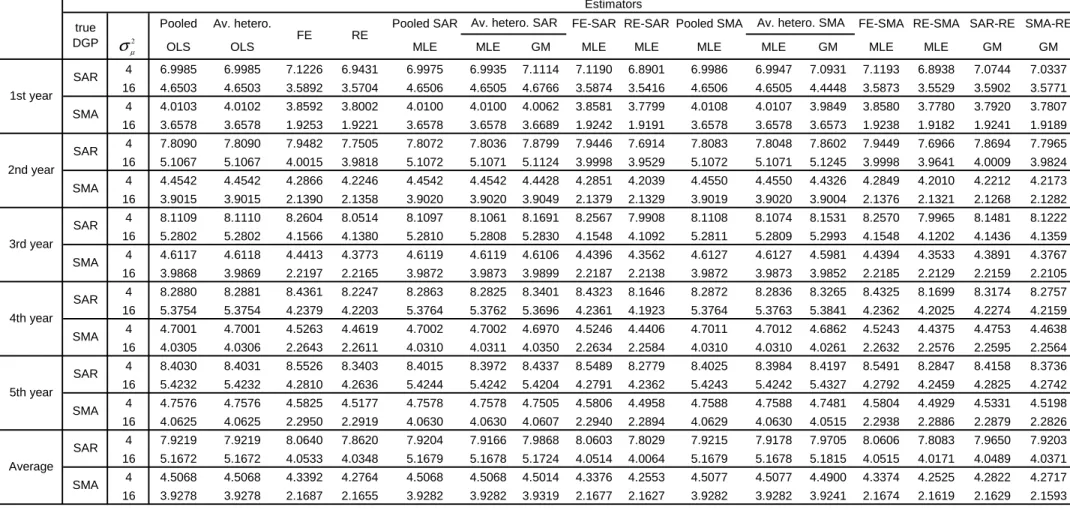
Tables 3 and 4 report the RMSE results as Tables

1

and 2 except that the

weight matrix is changed from a

W

(1

,

1)

to

W

(5

,

5)

,

i.e.,

fi

ve neighbors

behind and

fi

ve neighbors ahead. Except for the magnitudes of the RMSE,

the same rankings in terms of RMSE performance are exhibited as before.

Tables 5 and 6 report the RMSE results as Tables

1

and 2 except that

T

is

now doubled from

10

to

20

holding

N

fi

xed at

50

. Except for the magnitudes

of the RMSE, the same rankings in terms of RMSE performance are exhibited

as before.

Table 7 reports the RMSE results when

ρ

=

λ

= 0

.

8

,

the weight matrix

is

W

(1

,

1)

,

and

N

is doubled from

50

to

100

holding

T

fi

xed at

10

. While

Table 8 reports the RMSE results as Table 7 except that the weight matrix

is

W

(5

,

5)

.

Except for the magnitudes of the RMSE, the same rankings in

terms of RMSE performance are exhibited as before.

6

5.2.2

Sensitivity to Irregular Lattice Structures

The spatial weights matrices considered in the paper are regular lattice

struc-tures. Using real irregular lattices structures, as in Anselin and Moreno

(2003) and in Kelejian and Prucha (

1

999), does not change the conclusions

of the Monte Carlo study. We used real-world matrices by taking spatial

groupings of French administrative communes for dimension

N

= 50

.

7

Those

spatial matrices have been used by Baltagi, Bresson and Pirotte (2007).

Spa-tial weight matrices may represent high-order contiguity relationships. We

use a

k

-order contiguity matrix containing

N

₋

1

potential neighborhoods

in French municipalities. We have patterns of

0

and

1

values in an

(

N

₋

1)

by

(

N

₋

1)

grid for the

k

-nearest neighborhoods and we use the

1

-nearest

neighborhood

(

k

= 1)

and the

5

-nearest neighborhoods

(

k

= 1)

8

_{. Results of}

Tables 9 to

1

2 are very similar to those of Tables

1

to 4. Using irregular

lattice structures do not change the main conclusions in terms of the RMSE

forecast performance of the various estimators considered. These are similar

to the rankings obtained when regular lattice structures are used, only the

magnitudes of the RMSE di

ff

er.

5.2.3

Robustness to Non-Normality

So far, we have been assuming that the error components have been generated

by the normal distribution. In this section, we check the sensitivity of our

results to non-normal disturbances. In particular, we generate the

µ

_i

’s from

a

χ

2

_{distribution and we let the remainder disturbances follow the normal}

distribution. Tables

1

3 and

1

4 give similar results as those of Tables

1

and

2 (when the individual e

ff

ects follow a normal distribution). So, the results

seem to be robust to non-normality of the disturbances of the

χ

2

_type.

RMSE forecast performance and are not shown here to save space. These are available

upon request from the authors.

7

_{Other Tables for}

_N

_{= 100}

_{are available upon request from the authors.}

8

_{Note that a non-zero entry in row}

_i

_{, column}

_j

_{denotes that neighborhoods}

_i

_and

_j

_have

borders that touch and are therefore considered “neighbors”. For

N

= 50

and for

k

= 5

,

and for the

2401

possible elements in the

49

by

49

matrix, there are only

250

non-zero

elements. So, the sparseness value is

10%

(

= 250

/

2500

). These non-zero entries re

fl

ect the

contiguity relations between the

5

-nearest neighborhoods.

6

Summary and Conclusion

Our Monte Carlo study

fi

nds that when the true DGP is RE with a SAR or

SMA remainder disturbances, estimators that ignore heterogeneity/spatial

correlation perform badly in RMSE forecasts. For our experiments,

account-ing for heterogeneity improves the forecast performance by a big margin and

accounting for spatial correlation improves the forecast but by a smaller

mar-gin. Ignoring both leads to the worst forecasting performance. Heterogeneous

estimators based on averaging perform worse than homogeneous estimators

in forecasting performance. This performance improves with a larger

sam-ple size and seems robust to the type of spatial error structure imposed on

the remainder disturbances. These Monte Carlo experiments con

fi

rm earlier

empirical studies that report similar

fi

ndings.

7

Appendix

This appendix

fi

rst derives the BLUP for the KKP model which we are calling

the (SAR-RE) model described in (

1

3) and (

1

4). The variance-covariance

matrix

Ω

is given in (

1

7). The inverse of

Ω

is given by:

Ω

−1

=

1

σ

2 v

·µ

I

T

−

T

σ

2µ

σ

2 1

J

T

¶

⊗

(

B

_N0

B

N

)

¸

where

J

T

=

J

T

/T

and

σ

21

=

T

σ

2µ

+

σ

2v

and

B

N

= (

I

N

−

ρ

W

N

)

. From (

1

3)

and (

1

4), we have :

ε

T+τ

=

B

N−1

u

T+τ

=

B

−N1

(

µ

+

v

T+τ

)

so that,

E

h

ε

T+τ

ε

0

i

=

E

h

B

_N−1

(

µ

+

v

T+τ

)

¡¡

ι

T

⊗

B

N−1

¢

µ

+

¡

I

T

⊗

B

N−1

¢

v

¢

0

i

=

σ

2_µ

B

_N−1

³

ι

0_T

_⊗

B

_N−10

´

ω

0

=

E

h

ε

i,T+τ

ε

0

i

=

σ

2µ

b

i

³

ι

0T

⊗

B

− 10 N

´

where

b

i

is the

i

th row of the matrix

B

N−1

. In this case,

ω

0

Ω

−1

=

σ

2 µ

σ

2 v

b

i

³

ι

0_T

_⊗

B

_N−10

´ ·µ

I

T

−

T

σ

2µ

σ

2 1

J

T

¶

⊗

(

B

_N0

B

N

)

¸

=

σ

2 µ

σ

2 v

b

i

·³

ι

0_T

_⊗

B

N

´

−

T

σ

2 µ

σ

2 1

³

ι

0_T

_⊗

B

N

´¸

=

σ

2 µ

σ

2 1

b

i

³

ι

0_T

_⊗

B

N

´

But

b

i

¡

ι

0_T

_⊗

B

N

¢

= (1

_⊗

b

i)

¡

ι

0_T

_⊗

B

N

¢

=

¡

ι

0_T

_⊗

l

0 i

¢

, where

l

0 i

is the

i

th row of

I

N

. This holds because

B

N−1

B

N

=

I

N

and therefore

b

i

B

N

=

l

0i

. This means

that the predictor of the KKP model from (28) is given by:

b

y

i,T+τ

=

X

i,T+τ

β

b

GLS

+

σ

2µ

σ

2 1

(

ι

0_T

_⊗

l

_i0

)

_b

ε

GLS

(36)

which is the same as that of the RE model with no spatial correlation. While

the predictor formula is the same, the MLEs for these speci

fi

cations yield

di

ff

erent estimates which in turn yield di

ff

erent residuals and hence di

ff

erent

forecasts.

The proof is the similar for the Fingleton (2007) speci

fi

cation which we

are calling the (SMA-RE) model described in (25) and (

1

4). The

variance-covariance matrix

Ω

is given in (27). The inverse of

Ω

is given by:

Ω

−1

=

1

σ

2 v

·µ

I

T

−

T

σ

2µ

σ

2 1

J

T

¶

⊗

(

D

N

D

0N

)

−1

¸

where

D

N

= (

I

N

+

λ

W

N

)

. From (25) and (

1

4), we have :

ε

T+τ

=

D

N

u

T+τ

=

D

N

(

µ

+

v

T+τ

)

so that,

E

[

ε

T+τ

ε

0

] =

E

£

D

N

(

µ

+

v

T+τ

) ((

ι

T

⊗

D

N

)

µ

+ (

I

T

⊗

D

N

)

v

)

0

¤

=

σ

2_µ

D

N

³

ι

0_T

_⊗

D

_N0

´

ω

0

=

E

[

ε

i,T+τ

ε

0

] =

σ

2µ

d

i

³

ι

0_T

_⊗

D

0_N

´

where

d

i

is the

i

th row of the matrix

D

N

. In this case,

ω

0

Ω

−1

=

σ

2 µ

σ

2 v

d

i

³

ι

0_T

_⊗

D

0_N

´ ·µ

I

T

−

T

σ

2 µ

σ

2 1

J

T

¶

⊗

(

D

N

D

N0

)

−1

¸

=

σ

2 µ

σ

2 v

d

i

·³

ι

0_T

_⊗

D

_N−1

´

₋

T

σ

2 µ

σ

2 1

³

ι

0_T

_⊗

D

−_N1

´¸

=

σ

2 µ

σ

2 1

d

i

³

ι

0_T

_⊗

D

−_N1

´

But

d

i

¡

ι

0_T

_⊗

D

−_N1

¢

= (1

_⊗

d

i)

¡

ι

0_T

_⊗

D

_N−1

¢

=

¡

ι

0_T

_⊗

l

0 i

¢

, where

l

0 i

is the

i

th row of

I

N

. This holds because

D

N

D

−N1

=

I

N

and therefore

d

i

D

N−1

=

l

0i

. This means

that the predictor of the Fingleton (2007) model is again the same as that

of the RE model with no spatial correlation. While the predictor formula is

the same, the MLEs for these speci

fi

cations yield di

ff

erent estimates which

in turn yield di

ff

erent residuals and hence di

ff

erent forecasts.

References

Anselin, L.,

1

988, Spatial Econometrics: Methods and Models, Kluwer Academic

Pub-lishers, Dordrecht.

Anselin, L. and A.K. Bera,

1

998, Spatial dependence in linear regression models with an

introduction to spatial econometrics. In A. Ullah and D.E.A. Giles, eds., Handbook

of Applied Economic Statistics, Marcel Dekker, New York.

Anselin, L. and R. Moreno, 2003, Properties of tests for spatial error components,

Re-gional Science and Urban Economics 33, 595-6

1

8.

Anselin, L., J. Le Gallo and H. Jayet, 2008, Spatial panel econometrics. Ch.

1

9 in L.

Mátyás and P. Sevestre, eds., The Econometrics of Panel Data: Fundamentals and

Recent Developments in Theory and Practice, Springer-Verlag, Berlin, 625-660.

Baillie, R.T. and B.H. Baltagi,

1

999, Prediction from the regression model with one-way

error components, Chapter

1

0 in C. Hsiao, K. Lahiri, L.F. Lee and H. Pesaran, eds.,

Analysis of Panels and Limited Dependent Variable Models, Cambridge University

Press, Cambridge, 255—267.

Baltagi, B.H., 2008, Forecasting with panel data, Journal of Forecasting 27,

1

53-

1

73..

Baltagi, B.H. and J.M. Gri

ffi

n,

1

997, Pooled estimators vs. their heterogeneous

counter-parts in the context of dynamic demand for gasoline, Journal of Econometrics 77,

303—327.

Baltagi, B.H. and D. Li, 2004, Prediction in the panel data model with spatial correlation,

Chapter

1

3 in L. Anselin, R.J.G.M. Florax and S.J. Rey, eds., Advances in Spatial

Econometrics: Methodology, Tools and Applications, Springer, Berlin, 283—295.

Baltagi, B.H. and D. Li, 2006, Prediction in the panel data model with spatial correlation:

The case of liquor, Spatial Economic Analysis

1

,

1

75-

1

85.

Baltagi, B.H. and Q. Li,

1

992, Prediction in the one-way error component model with

serial correlation, Journal of Forecasting

11

, 56

1

—567.

Baltagi, B.H., G. Bresson and A. Pirotte, 2002, Comparison of forecast performance for

homogeneous, heterogeneous and shrinkage estimators: Some empirical evidence

from US electricity and natural-gas consumption, Economics Letters 76, 375-382.

Baltagi, B.H., G. Bresson and A. Pirotte, 2004, Tobin q: forecast performance for

hier-archical Bayes, shrinkage, heterogeneous and homogeneous panel data estimators,

Empirical Economics 29,

1

07-

11

3.

Baltagi, B.H., G. Bresson and A. Pirotte, 2007, Panel unit root tests and spatial

depen-dence, Journal of Applied Econometrics 22, 339-360.

Baltagi, B.H., J.M. Gri

ffi

n and W. Xiong, 2000, To pool or not to pool: Homogeneous

versus heterogeneous estimators applied to cigarette demand, Review of Economics

and Statistics 82,

11

7—

1

26.

Brucker, H. and B. Siliverstovs, 2006, On the estimation and forecasting of international

migration: how relevant is heterogeneity across countries, Empirical Economics 3

1

,

735-754.

Fingleton, B., 2007a, A generalized method of moments estimator for a spatial model with

endogenous spatial lag and spatial moving average errors, paper presented at the

1

3th international conference on panel data, University of Cambridge, forthcoming

Spatial Economic Analysis.

Fingleton, B., 2007b, A generalized method of moments estimator for a spatial model

with moving average errors with application to real estate prices, forthcoming in

Empirical Economics.

Frees, E.W. and T.W. Miller, 2004, Sales forecasting using longitudinal data models.

International Journal of Forecasting 20, 99—

11

4.

Goldberger, A.S.,

1

962, Best linear unbiased prediction in the generalized linear

regres-sion model, Journal of the American Statistical Association 57, 369—375.

Kapoor, M., H.H. Kelejian and I.R. Prucha, 2007, Panel data models with spatially

correlated error components, Journal of Econometrics

1

40, 97-

1

30.

Kelejian, H.H. and I.R. Prucha,

1

999, A generalized moments estimator for the

autore-gressive parameter in a spatial model, International Economic Review 40, 509-533.

Lee, L.F. and W.E. Gri

ffi

ths,

1

979, The prior likelihood and best linear unbiased

pre-diction in stochastic coe

ffi

cient linear models, working paper, Department of

Eco-nomics, University of Minnesota.

Hoogstrate, A.J., F.C. Palm and G.A. Pfann, 2000, Pooling in dynamic panel-data

mod-els: An application to forecasting GDP growth rates, Journal of Business and

Eco-nomic Statistics

1

8, 274-283.

Hsiao, C. and A.K. Tahmiscioglu,

1

997, A panel analysis of liquidity constraints and

fi

rm

investment, Journal of the American Statistical Association 92, 455—465.

Nerlove, M.,

1

97

1

, Futher evidence on the estimation of dynamic economic relations from

a time-series of cross-sections, Econometrica 39, 359-382.

Pesaran, M.H. and R. Smith,

1

995, Estimating long-run relationships from dynamic

heterogenous panels, Journal of Econometrics 68, 79—

11

3.

Rapach, D.E. and M.E. Wohar, 2004, Testing the monetary model of exchange rate

determination: a closer look at panels, Journal of International Money and Finance

23, 867—895.

Schmalensee, R., T.M. Stoker and R.A. Judson,

1

998, World carbon dioxide emissions:

1

950-2050, Review of Economics and Statistics 80,

1

5—27.

Spanos, A., 2002, The ET interview: Professor Phoebus J. Dhrymes, Econometric Theory

1

8,

1

22

1

-

1

272.

Taub, A.J.,

1

979, Prediction in the context of the variance-components model, Journal

of Econometrics

1

0,

1

03—

1

08.

Theil, H.,

1

96

1

, Economic Forecasts and Policy, North-Holland, Amsterdam.

Wansbeek, T.J. and A. Kapteyn,

1

978, The seperation of individual variation and

sys-tematic change in the analysis of panel data, Annales de l’INSEE 30-3

1

, 659-680.

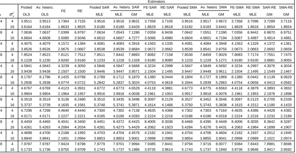
Pooled Av. hetero. Pooled SAR FE-SAR RE-SAR Pooled SMA FE-SMA RE-SMA SAR-RE SMA-RE

ρ OLS OLS MLE MLE GM MLE MLE MLE MLE GM MLE MLE GM GM

0.4 4 3.9781 3.9782 3.8102 3.7645 3.9781 3.9781 3.9606 3.8093 3.7558 3.9782 3.9782 3.9464 3.8093 3.7558 3.7610 3.7765 16 3.6289 3.6290 1.9019 1.8989 3.6300 3.6299 3.6522 1.9007 1.8971 3.6301 3.6300 3.6569 1.9007 1.8973 1.8978 1.9134 0.8 4 7.0556 7.0552 7.1957 7.0218 7.0529 7.0389 7.0558 7.1917 6.9564 7.0541 7.0403 7.0796 7.1917 6.9668 7.0187 7.0382 16 4.6529 4.6533 3.5908 3.5764 4.6584 4.6569 4.6697 3.5863 3.5518 4.6589 4.6576 4.6644 3.5867 3.5603 3.6047 3.5908 0.4 4 4.4164 4.4165 4.2360 4.1840 4.4162 4.4162 4.3423 4.2354 4.1763 4.4164 4.4164 4.3721 4.2353 4.1755 4.1808 4.1739 16 3.8731 3.8733 2.1207 2.1175 3.8742 3.8743 3.8849 2.1194 2.1155 3.8742 3.8744 3.8918 2.1195 2.1156 2.1164 2.1216 0.8 4 7.8106 7.8106 7.9469 7.7633 7.8066 7.7911 7.8100 7.9408 7.6956 7.8073 7.7920 7.8306 7.9407 7.7034 7.7832 7.8190 16 5.1174 5.1177 4.0090 3.9942 5.1221 5.1209 5.1206 4.0039 3.9661 5.1225 5.1213 5.1084 4.0042 3.9754 3.9923 3.9833 0.4 4 4.5807 4.5808 4.3992 4.3445 4.5805 4.5805 4.5627 4.3986 4.3364 4.5806 4.5807 4.5560 4.3985 4.3357 4.3414 4.3475 16 3.9582 3.9585 2.2004 2.1972 3.9591 3.9592 3.9660 2.1992 2.1954 3.9591 3.9594 3.9682 2.1993 2.1956 2.1963 2.2023 0.8 4 8.1467 8.1467 8.2921 8.1023 8.1424 8.1273 8.1458 8.2853 8.0289 8.1430 8.1279 8.1618 8.2854 8.0382 8.1016 8.1402 16 5.2892 5.2894 4.1685 4.1529 5.2936 5.2923 5.2763 4.1636 4.1234 5.2940 5.2928 5.2674 4.1640 4.1337 4.1387 4.1450 0.4 4 4.6719 4.6720 4.4891 4.4335 4.6718 4.6717 4.6676 4.4882 4.4250 4.6719 4.6720 4.6583 4.4881 4.4245 4.4301 4.4332 16 4.0024 4.0026 2.2471 2.2440 4.0031 4.0033 4.0117 2.2460 2.2423 4.0032 4.0034 4.0125 2.2461 2.2424 2.2432 2.2451 0.8 4 8.3035 8.3035 8.4435 8.2560 8.2997 8.2836 8.3011 8.4367 8.1826 8.3005 8.2843 8.3225 8.4370 8.1922 8.3142 8.3214 16 5.3799 5.3802 4.2531 4.2377 5.3838 5.3826 5.3662 4.2481 4.2085 5.3841 5.3829 5.3626 4.2485 4.2183 4.2296 4.2143 0.4 4 4.7238 4.7239 4.5443 4.4870 4.7238 4.7238 4.7274 4.5432 4.4778 4.7239 4.7240 4.7199 4.5432 4.4775 4.4836 4.4906 16 4.0283 4.0285 2.2727 2.2698 4.0288 4.0290 4.0362 2.2716 2.2681 4.0289 4.0291 4.0374 2.2716 2.2682 2.2689 2.2718 0.8 4 8.4195 8.4197 8.5680 8.3756 8.4158 8.3995 8.4173 8.5606 8.2997 8.4164 8.4001 8.4331 8.5608 8.3100 8.4299 8.4256 16 5.4280 5.4282 4.2962 4.2812 5.4313 5.4301 5.4156 4.2911 4.2526 5.4317 5.4305 5.4125 4.2914 4.2618 4.2808 4.2710 0.4 4 4.4742 4.4743 4.2957 4.2427 4.4741 4.4740 4.4601 4.2949 4.2343 4.4742 4.4743 4.4505 4.2949 4.2338 4.2394 4.2444 16 3.8982 3.8984 2.1486 2.1455 3.8990 3.8992 3.9102 2.1474 2.1437 3.8991 3.8993 3.9133 2.1474 2.1438 2.1445 2.1509 Estimators

Table 1 - Forecasts RMSE - (N,T)=(50,10), SAR data generating process for φφφφ, W(1,1), 1000 replications

FE RE

Av. hetero. SAR Av. hetero. SMA

Average 1st year 2nd year 3rd year 4th year 5th year 2 µ

σ

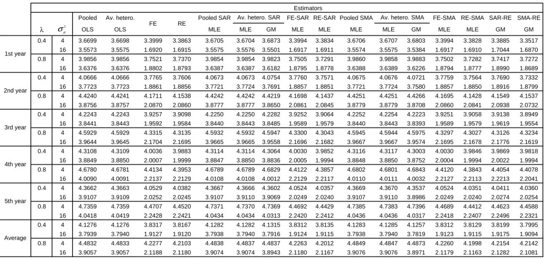
Pooled Av. hetero. Pooled SAR FE-SAR RE-SAR Pooled SMA FE-SMA RE-SMA SAR-RE SMA-RE

λ OLS OLS MLE MLE GM MLE MLE MLE MLE GM MLE MLE GM GM

0.4 4 3.6702 3.6703 3.4717 3.4261 3.6704 3.6701 3.6706 3.4707 3.4193 3.6705 3.6702 3.6669 3.4707 3.4187 3.4330 3.4375 16 3.5582 3.5582 1.7481 1.7455 3.5583 3.5584 3.5606 1.7478 1.7450 3.5584 3.5585 3.5569 1.7479 1.7449 1.7444 1.7323 0.8 4 3.9870 3.9873 3.8507 3.7906 3.9857 3.9856 3.9878 3.8481 3.7653 3.9858 3.9859 3.9770 3.8480 3.7635 3.7915 3.8213 16 3.6364 3.6364 1.9117 1.9095 3.6381 3.6377 3.6235 1.9098 1.9068 3.6380 3.6376 3.6316 1.9097 1.9062 1.9270 1.9078 0.4 4 4.0793 4.0793 3.8608 3.8133 4.0794 4.0792 4.0796 3.8600 3.8060 4.0795 4.0793 4.0816 3.8600 3.8056 3.8269 3.8097 16 3.7747 3.7748 1.9380 1.9354 3.7751 3.7754 3.7756 1.9375 1.9346 3.7752 3.7755 3.7759 1.9376 1.9345 1.9282 1.9255 0.8 4 4.4390 4.4391 4.2819 4.2224 4.4388 4.4386 4.4209 4.2783 4.1971 4.4396 4.4396 4.4105 4.2777 4.1952 4.2168 4.2313 16 3.8696 3.8697 2.1223 2.1191 3.8716 3.8714 3.8791 2.1201 2.1157 3.8718 3.8717 3.8821 2.1199 2.1149 2.1374 2.1270 0.4 4 4.2357 4.2358 4.0121 3.9644 4.2358 4.2358 4.2367 4.0111 3.9563 4.2360 4.2359 4.2393 4.0111 3.9560 3.9785 3.9661 16 3.8526 3.8527 2.0109 2.0084 3.8531 3.8534 3.8521 2.0104 2.0074 3.8531 3.8535 3.8537 2.0104 2.0074 2.0076 2.0047 0.8 4 4.6176 4.6177 4.4527 4.3926 4.6176 4.6175 4.5966 4.4490 4.3684 4.6184 4.6184 4.5887 4.4483 4.3652 4.3835 4.3981 16 3.9613 3.9614 2.2116 2.2084 3.9636 3.9634 3.9673 2.2095 2.2054 3.9638 3.9636 3.9692 2.2094 2.2045 2.2194 2.2168 0.4 4 4.3113 4.3114 4.0834 4.0354 4.3110 4.3111 4.3131 4.0823 4.0263 4.3112 4.3112 4.3161 4.0823 4.0263 4.0608 4.0475 16 3.8901 3.8902 2.0500 2.0474 3.8905 3.8908 3.8901 2.0494 2.0464 3.8906 3.8909 3.8917 2.0494 2.0463 2.0465 2.0482 0.8 4 4.7133 4.7133 4.5470 4.4856 4.7135 4.7134 4.6870 4.5433 4.4613 4.7146 4.7144 4.6837 4.5428 4.4581 4.4617 4.4901 16 4.0100 4.0101 2.2659 2.2627 4.0122 4.0121 4.0134 2.2642 2.2598 4.0123 4.0122 4.0152 2.2639 2.2590 2.2619 2.2631 0.4 4 4.3637 4.3638 4.1367 4.0876 4.3635 4.3635 4.3653 4.1357 4.0786 4.3637 4.3637 4.3695 4.1357 4.0786 4.1094 4.0975 16 3.9122 3.9124 2.0748 2.0722 3.9126 3.9129 3.9147 2.0743 2.0712 3.9127 3.9131 3.9147 2.0742 2.0711 2.0729 2.0752 0.8 4 4.7697 4.7698 4.6004 4.5394 4.7702 4.7700 4.7457 4.5967 4.5160 4.7713 4.7712 4.7428 4.5963 4.5125 4.5223 4.5371 16 4.0405 4.0405 2.2956 2.2926 4.0426 4.0425 4.0396 2.2937 2.2898 4.0428 4.0427 4.0411 2.2934 2.2889 2.2890 2.2901 0.4 4 4.1321 4.1321 3.9129 3.8653 4.1320 4.1319 4.1331 3.9120 3.8573 4.1322 4.1320 4.1347 3.9120 3.8570 3.8817 3.8717 16 3.7976 3.7977 1.9644 1.9618 3.7979 3.7982 3.7986 1.9639 1.9609 3.7980 3.7983 3.7986 1.9639 1.9608 1.9599 1.9572 Estimators

Table 2 - Forecasts RMSE - (N,T)=(50,10), SMA data generating process for φφφφ, W(1,1), 1000 replications

FE RE

Av. hetero. SMA Av. hetero. SAR

5th year Average 1st year 2nd year 3rd year 4th year 2 µ

σ