An index-based short-form of the WISC-IV with accompanying analysis of the reliability and abnormality of differences

An index-based short-form of the WISC-IV with

accompanying analysis of the reliability and

abnormality of differences

John R. Crawford

*, Vicki Anderson

, Peter M. Rankin

and Jayne MacDonald

1

_{School of Psychology, University of Aberdeen, UK}

_{Royal Children’s Hospital, Melbourne, Australia}

_{University of Melbourne, Australia}

4

_{Department of Psychological Medicine, Great Ormond Street Hospital}

for Children NHS Trust, London, UK

Objectives. To develop an Index-based, seven subtest, short-form of the Wechsler intelligence scale for children fourth edition (WISC-IV) that offers the same comprehensive range of analytic methods available for the full-length version. Design and methods. Psychometric.

Results. The short-form Indexes had high reliability and criterion validity. Scores are expressed as Index scores and as percentiles. Methods are provided that allow setting of confidence limits on scores, and analysis of the reliability and abnormality of Index score differences. The use of the short-form is illustrated with a case example. A computer programme (that automates scoring and implements all the analytical methods) accompanies this paper and can be downloaded from the following web address: http://www.abdn.ac.uk/,psy086/dept/sf_wisc4.htm.

Conclusions. The short-form will be useful when pressure of time or client fatigue precludes use of a full-length WISC-IV. The accompanying computer programme scores and analyses an individual’s performance on the short-form instantaneously and minimizes the chance of clerical error.

Like its predecessors, the Wechsler Intelligence Scale for Children Fourth Edition (WISC-IV; Wechsler, 2003a) continues to serve as a workhorse of cognitive assessment in clinical research and practice. Time constraints and potential problems with patient fatigue mean that a short-form version of the WISC-IV is often required. Four principal approaches to the development of short-forms can be delineated. In the Satz-Mogel

* Correspondence should be addressed to Professor John R. Crawford, School of Psychology, College of Life Sciences and Medicine, King’s College, University of Aberdeen, Aberdeen AB24 3HN, UK (e-mail: [email protected]).

The British Psychological Society

British Journal of Clinical Psychology (2010), 49, 235–258 q2010 The British Psychological Society

www.bpsjournals.co.uk

approach (e.g. Satz & Mogel, 1962), which is perhaps the most radical method, all subtests are administered but every second or third test item is omitted. It could be argued that this is a wasteful approach because all subtests are not created equal: some are more reliable, valid, and practical indicators of the ability dimensions or factors that underlie WISC-IV performance. Thus, when time is limited, there is a case for focusing on these subtests rather than spreading effort widely but thinly.

The three remaining approaches all omit subtests but differ in how the short-form is constructed. Probably the most widely adopted approach is to prorate omitted subtests (i.e. substitute the mean score on those subtests administered for those omitted) and thereafter proceed as though the full-length version had been given. Yet another alternative is to build regression equations to predict full-length IQs or Index scores from a subset of the subtests (Crawford, Allan, & Jack, 1992; Reynolds, Willson, & Clark, 1983). The fourth approach, and the one adopted here, is that originally proposed by Tellegen and Briggs (1967); see also Atkinson (1991) for an example of its application to the Wechsler Adult Intelligence Scale Revised (WAIS-R), and Crawford, Allum, and Kinion (2008a) for its application to the Wechsler Adult Intelligence Scale Third Edition (WAIS-III). With this approach, the subtests selected for the short-form are combined into composites and the composite scores transformed to an IQ metric (i.e. mean 100 and standard deviation 15). Thus the aim is not to predict full-length IQs or Indexes but to treat the composites as free standing measures of ability. This does not mean that criterion validity is necessarily ignored: for example, subtests could be selected to maximize the correlation between the short-form IQ or Indexes and their full-length counterparts.

This latter approach has a very significant advantage: it is relatively simple to provide all the additional information required to conduct the same forms of quantitative analysis on the short-form scores as is available for the full-length WISC-IV (Crawford

et al., 2008a). This is in marked contrast to the other methods of forming short-forms. Taking prorating as an example: the reliability of prorated IQs or Indexes will differ from their full-length counterparts, thereby invalidating the use of confidence intervals on scores derived from the full-length version. The differences in reliabilities also invalidate the use of the tabled values in the WISC-IV manual (Table B.1) when attempting to test for reliable differences between a child’s Index scores. Moreover, for the full-length WISC-IV, analysis of the abnormality of differences among a child’s Index scores can be conducted using a table of the base-rates for differences in the standardization sample (Table B.2). The use of this table with prorated scores is questionable because (a) the correlations between the prorated Indexes will differ from their full-length counterparts, and (b) these correlations determine the level of abnormality of any differences (Crawford, Garthwaite, & Gault, 2007). With the approach used in the present study all of these problems are overcome by calculating the reliabilities and intercorrelations of the indexes from the statistics of the subtests contributing to them. Turning now to the selection of subtests for the short-form, the primary consideration was that the form should provide index scores as well as a short-form full scale IQ. Index scores reflect the underlying factor structure of the WISC-IV and therefore have high construct validity. So that there would be significant time savings when using the short-form we limited it to seven subtests: there were two indicators each for three of the WISC-IV indexes and one for the Working Memory (WM) Index.

Vocabulary and Similarities were selected for the Verbal Comprehension (VC) Index: Vocabulary is highly reliable and has the highest loading on the VC factor (Wechsler, 2003a), Similarities has a slightly lower loading on the VC factor than Comprehension

(0.74 vs. 0.78 averaged over all ages) but is more reliable (0.86 vs. 0.81 averaged over all ages) (Wechsler, 2003a) and is a useful measure of the ability to engage in basic abstract verbal reasoning. Block Design and Matrix Reasoning were selected for the Perceptual Reasoning (PR) Index: these subtests have higher reliabilities and higher loadings on the PR factor than Picture Concepts.

Selection of subtests for the remaining two indexes is more contentious (in particular the choice of two subtests for Processing Speed (PS) and one for WM rather than the other way round) and it may be that other neuropsychologists would favour an alternative selection. The selection was largely based on the practical problems experienced with Letter-Number Sequencing (in our experience many children encountered in clinical practice find it confusing). Thus Digit Span was used as the sole subtest for the WM Index (these two subtest have equivalent loadings on the WM factor), and both PS subtests (Coding and Symbol Search) were used for the PS Index. The methods used to build and analyse the short-form follow those developed by Crawford et al. (2008a) for the WAIS-III. A reasonable amount of technical detail is provided because we considered it important that potential users of the short-form should be fully informed of the methods that underlie the results it provides. In addition, the level of detail is such that the methods could readily be adopted by others to create alternative WISC-IV short-forms. Finally, this paper contains all the information required to score and conduct a basic analysis of a child’s short-form scores. However, we have also developed a computer programme to automate this process. The programme provides a convenient alternative to hand scoring and reduces the chance of clerical error. It also provides some additional analysis options (see later section for details).

Method and results

Building the index-based short-form

The first step in developing short-forms of the indexes is to determine the means and standard deviation of the composites. The means are obtained simply by multiplying the number of subtests in each composite by 10 (the mean of an individual WISC-IV subtest); thus, for the VC composite, the mean is 20, and for Full Scale IQ (FSIQ), the mean is 70. The standard deviation of a composite is a function of the standard deviations of the individual components (i.e. the subtests) and their intercorrelations (the WISC-IV subtest correlation matrix is presented in Table 5.1 of the technical and interpretive manual). The simplest way of obtaining this standard deviation is to form a variance– covariance matrix (the covariance is obtained by multiplying each correlation by the standard deviations of the relevant pairs of components; in the present case, because the subtests have a common standard deviation of 3, the correlation is simply multiplied by 9). For example, from the WISC-IV technical and interpretive manual, the correlation between Vocabulary and Similarities is 0.74 and thus the covariance is 6.66. The sum of the elements in this variance–covariance matrix (9þ6:66þ9þ6:66¼31:32) is the variance of the composite and by taking the square root of this we obtain the standard deviation of the composite (5.596 in this case).

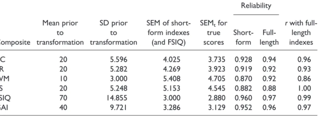
The means and standard deviations of the five composites are presented in Table 1, note that the WM ‘composite’ consists only of Digit Span and thus the mean and standard deviation are simply 10 and 3, respectively. Note that this table also reports the equivalent statistics for the short-form FSIQ and for a further index, the General Ability Index (GAI); discussion of this latter index is deferred until a later section.

Having obtained the means and standard deviations of the composites, we now have the constants required to be able to transform each of the composite scores to have a mean and standard deviation of 100 and 15, respectively. The generic formula is:

Xnew¼s_snew

old Xold2

{

Xold þX{new; ð1Þ

where Xnew is the transformed score, Xold is the original score, sold is the standard

deviation of the original scale,snewis the standard deviation of the scale you wish to

convert to,X{oldis the mean of the original scale, andX{new is the mean of the scale you

wish to convert to.

Thus for example, if the sum of a child’s subtest scores on Vocabulary and Similarities is 15 then the short-form VC Index score is 87 after rounding. Formula (1) was used to generate the tables for conversion of the sums of subtest scores to short-form index scores and FSIQs (Tables 2–7) and is also used in the computer programme that accompanies this paper. For the full-length indexes, scores are also expressed as percentiles. Therefore, in keeping with the aim of providing equivalent information for the short-form indexes, percentile norms are also presented in Tables 2–7 and are provided by the computer programme. To express the scores as percentiles, index scores were expressed as z, and the probabilities corresponding to these quantiles multiplied by 100. Thus for example, thez for an index score of 115 isþ1.0 and the score is thus at the 84th percentile. In Tables 2–7 percentiles are expressed as integers unless the index score is very extreme (i.e. below the 1st or above the 99th percentile) in which case they are presented to one decimal place.

Reliabilities and standard errors of measurement for the short-form indexes

In order to set confidence limits on a child’s score on the short-form indexes, and to test whether a child exhibits reliable differences between her/his short-form index scores, it is necessary to obtain the standard error of measurement for each short-form index. To obtain this statistic we first need to obtain the reliability of the short-form indexes. Of course the reliability of the short-form is also an important piece of information in its own right; measures with low reliability should be avoided, particularly when the concern is with assessing anindividualchild’s performance (Crawford, 2004).

Table 1.Summary statistics and basic psychometric properties of the index-based short-form of the WISC-IV Reliability Composite Mean prior to transformation SD prior to transformation SEM of short-form indexes (and FSIQ) SEMtfor true

scores Short-form length

Full-rwith full-length indexes VC 20 5.596 4.025 3.735 0.928 0.94 0.96 PR 20 5.282 4.269 3.923 0.919 0.92 0.93 WM 10 3.000 5.408 4.705 0.870 0.92 0.86 PS 20 5.248 5.153 4.545 0.882 0.88 1.00 FSIQ 70 14.855 3.000 2.880 0.960 0.97 0.99 GAI 40 9.721 3.286 3.129 0.952 0.96 0.97

When, as in the present case, the components have equal means and standard deviations, and are given equal weights in determining the composite score, the reliability of a composite is a simple function of the reliabilities of the components (i.e. subtests) and their intercorrelations (the higher the intercorrelations between

Table 2.Table for converting the sum of subtest scores (SSS) on theVocabularyandSimilaritiessubtests toVCshort-form index scores and estimated true scores; 95% confidence limits on obtained index scores are also provided (limits on true scores are in brackets) as is the percentile corresponding to each index score

95% CLs

SSS Index score Est true score Percentile Lower limit Upper limit

2 52 55 ,0.1 44 (48) 60 (63) 3 54 58 0.1 47 (50) 62 (65) 4 57 60 0.2 49 (53) 65 (68) 5 60 63 0.4 52 (55) 68 (70) 6 62 65 0.6 55 (58) 70 (72) 7 65 68 1.0 57 (60) 73 (75) 8 68 70 2 60 (63) 76 (77) 9 71 73 3 63 (65) 78 (80) 10 73 75 4 65 (68) 81 (82) 11 76 78 5 68 (70) 84 (85) 12 79 80 8 71 (73) 86 (87) 13 81 83 10 73 (75) 89 (90) 14 84 85 14 76 (78) 92 (92) 15 87 88 19 79 (80) 94 (95) 16 89 90 23 81 (83) 97 (97) 17 92 93 30 84 (85) 100 (100) 18 95 95 37 87 (88) 103 (102) 19 97 98 42 89 (90) 105 (105) 20 100 100 50 92 (93) 108 (107) 21 103 102 58 95 (95) 111 (110) 22 105 105 63 97 (98) 113 (112) 23 108 107 70 100 (100) 116 (115) 24 111 110 77 103 (103) 119 (117) 25 113 112 81 106 (105) 121 (120) 26 116 115 86 108 (108) 124 (122) 27 119 117 90 111 (110) 127 (125) 28 121 120 92 114 (113) 129 (127) 29 124 122 95 116 (115) 132 (130) 30 127 125 96 119 (118) 135 (132) 31 129 127 97 122 (120) 137 (135) 32 132 130 98 124 (123) 140 (137) 33 135 132 99.0 127 (125) 143 (140) 34 138 135 99.4 130 (128) 145 (142) 35 140 137 99.6 132 (130) 148 (145) 36 143 140 99.8 135 (132) 151 (147) 37 146 142 99.9 138 (135) 153 (150) 38 148 145 .99.9 140 (137) 156 (152)

components, the higher the reliability of the composite). The formula is:

rYY ¼12k2{_RSrXX

Y ; ð2Þ

where_{ kis the number of components,rXXare the reliabilities of the components and

RY is the sum of elements of the correlation matrix for the components (including the unities in the diagonal).

Table 3.Table for converting the SSS on theBlock DesignandMatrix Reasoningsubtests toPR short-form index scores and estimated true scores; 95% confidence limits on obtained index scores are also provided (limits on true scores are in brackets) as is the percentile corresponding to each index score

95% CLs

SSS Index score Est true score Percentile Lower limit Upper limit

2 49 53 ,0.1 41 (45) 57 (61) 3 52 56 ,0.1 43 (48) 60 (63) 4 55 58 0.1 46 (51) 63 (66) 5 57 61 0.2 49 (53) 66 (69) 6 60 63 0.4 52 (56) 69 (71) 7 63 66 0.7 55 (58) 71 (74) 8 66 69 1 58 (61) 74 (76) 9 69 71 2 60 (64) 77 (79) 10 72 74 3 63 (66) 80 (82) 11 74 77 4 66 (69) 83 (84) 12 77 79 6 69 (71) 86 (87) 13 80 82 9 72 (74) 88 (89) 14 83 84 13 75 (77) 91 (92) 15 86 87 18 77 (79) 94 (95) 16 89 90 23 80 (82) 97 (97) 17 91 92 27 83 (84) 100 (100) 18 94 95 34 86 (87) 103 (102) 19 97 97 42 89 (90) 106 (105) 20 100 100 50 92 (92) 108 (108) 21 103 103 58 94 (95) 111 (110) 22 106 105 66 97 (98) 114 (113) 23 109 108 73 100 (100) 117 (116) 24 111 110 77 103 (103) 120 (118) 25 114 113 82 106 (105) 123 (121) 26 117 116 87 109 (108) 125 (123) 27 120 118 91 112 (111) 128 (126) 28 123 121 94 114 (113) 131 (129) 29 126 123 96 117 (116) 134 (131) 30 128 126 97 120 (118) 137 (134) 31 131 129 98 123 (121) 140 (136) 32 134 131 99 126 (124) 142 (139) 33 137 134 99.3 129 (126) 145 (142) 34 140 137 99.6 131 (129) 148 (144) 35 143 139 99.8 134 (131) 151 (147) 36 145 142 99.9 137 (134) 154 (149) 37 148 144 .99.9 140 (137) 157 (152) 38 151 147 .99.9 143 (139) 159 (155)

The reliabilities of the short-form indexes calculated by this method are presented in Table 1; the reliabilities of the corresponding full-length indexes are also presented for comparison purposes (these latter reliabilities are from Table 4.1 of the WISC-IV technical manual). It can be seen that the reliabilities of the short-form indexes are all very high and, with the exception of WM, only marginally lower than the reliabilities of their full-length equivalents (the very modest reduction in reliability when moving from a full-length to short-form index can be attributed to the fact that those subtests selected for inclusion in the short-form had, in most cases, higher reliabilities and higher intercorrelations than those omitted).

Having obtained the reliabilities of the short-form indexes, the next stage is to calculate their standard errors of measurement. The formula for the standard error of measurement is:

SEMX¼sXpffiffiffiffiffiffiffiffiffiffiffiffiffiffiffiffi12rXX; ð3Þ wheresXis the standard deviation of the index scores and is therefore 15. The standard

errors of measurement for the short-form indexes are presented in Table 1. In the present case, we also compute and report (Table 1) the standard errors of measurement for scores expressed on a true score metric (see the WISC-IV technical manual for the required formula required and for further technical details). These two forms of standard errors will be used to provide alternative means of (a) setting confidence limits on index scores, and (b) testing for reliable differences between index scores (see later).

Table 4.Table for converting scores (SSS) on theDigit Spansubtest toWMshort-form index scores and estimated true scores; 95% confidence limits on obtained index scores are also provided (limits on true scores are in brackets) as is the percentile corresponding to each index score

95% CLs

SSS Index score True score Percentiles Lower limit Upper limit

1 55 61 0.1 44 (52) 66 (70) 2 60 65 0.4 49 (56) 71 (74) 3 65 70 1.0 54 (60) 76 (79) 4 70 74 2 59 (65) 81 (83) 5 75 78 5 64 (69) 86 (87) 6 80 83 9 69 (73) 91 (92) 7 85 87 16 74 (78) 96 (96) 8 90 91 25 79 (82) 101 (101) 9 95 96 37 84 (86) 106 (105) 10 100 100 50 89 (91) 111 (109) 11 105 104 63 94 (95) 116 (114) 12 110 109 75 99 (99) 121 (118) 13 115 113 84 104 (104) 126 (122) 14 120 117 91 109 (108) 131 (127) 15 125 122 95 114 (113) 136 (131) 16 130 126 98 119 (117) 141 (135) 17 135 130 99.0 124 (121) 146 (140) 18 140 135 99.6 129 (126) 151 (144) 19 145 139 99.9 134 (130) 156 (148)

Intercorrelations of the short-form indexes and correlations with their full-length equivalents

When attempting to detect acquired impairments, it is important to quantify the degree of abnormality of any differences in a child’s index score profile. Quantifying the abnormality of differences requires the standard deviation of the differences between each of the indexes, which in turn, requires knowledge of the correlations between the

Table 5.Table for converting the SSS onCodingandSymbol SearchtoPSshort-form index scores and estimated true scores; 95% confidence limits on obtained index scores are also provided (limits on true scores are in brackets) as is the percentile corresponding to each index score

95% CLs

SSS Index score True score Percentiles Lower limit Upper limit

2 49 55 ,0.1 38 (46) 59 (64) 3 51 57 ,0.1 41 (48) 62 (66) 4 54 60 0.1 44 (51) 64 (69) 5 57 62 0.2 47 (53) 67 (71) 6 60 65 0.4 50 (56) 70 (74) 7 63 67 0.7 53 (58) 73 (76) 8 66 70 1 56 (61) 76 (79) 9 69 72 2 58 (63) 79 (81) 10 71 75 3 61 (66) 82 (84) 11 74 77 4 64 (68) 84 (86) 12 77 80 6 67 (71) 87 (89) 13 80 82 9 70 (73) 90 (91) 14 83 85 13 73 (76) 93 (94) 15 86 87 18 76 (78) 96 (96) 16 89 90 23 78 (81) 99 (99) 17 91 92 27 81 (84) 102 (101) 18 94 95 34 84 (86) 104 (104) 19 97 97 42 87 (89) 107 (106) 20 100 100 50 90 (91) 110 (109) 21 103 103 58 93 (94) 113 (111) 22 106 105 66 96 (96) 116 (114) 23 109 108 73 98 (99) 119 (116) 24 111 110 77 101 (101) 122 (119) 25 114 113 82 104 (104) 124 (122) 26 117 115 87 107 (106) 127 (124) 27 120 118 91 110 (109) 130 (127) 28 123 120 94 113 (111) 133 (129) 29 126 123 96 116 (114) 136 (132) 30 129 125 97 118 (116) 139 (134) 31 131 128 98 121 (119) 142 (137) 32 134 130 99 124 (121) 144 (139) 33 137 133 99.3 127 (124) 147 (142) 34 140 135 99.6 130 (126) 150 (144) 35 143 138 99.8 133 (129) 153 (147) 36 146 140 99.9 136 (131) 156 (149) 37 149 143 .99.9 138 (134) 159 (152) 38 151 145 .99.9 141 (136) 162 (154)

indexes. These correlations can be calculated from the matrix of correlations between the subtests contributing to the indexes from the formula:

rXY ¼ { RXY ffiffiffiffiffiffiffi_{ RX p ffiffiffiffiffiffiffi_{ RY p ; ð4Þ

whereRXY{ is the sum of the correlations of each variable in compositeX(e.g. the VC short-form) with each variable in compositeY(e.g. the PR short-form), andRX{ andRY{ Table 6.Table for converting the SSS on all seven subtests to short-formFSIQscores and estimated true scores; 95% confidence limits on obtained FSIQ scores are also provided as is the percentile corresponding to each score—part 1

95% CLs 95% CLs

SSS IQ ETS Pcile L U SSS IQ ETS Pcile L U

7 37 39 ,0.1 31 42 43 73 74 4 67 79 8 38 40 ,0.1 32 43 44 74 75 4 68 80 9 39 41 ,0.1 33 44 45 75 76 5 69 81 10 40 42 ,0.1 34 45 46 76 77 5 70 82 11 41 43 ,0.1 35 46 47 77 78 6 71 83 12 42 44 ,0.1 36 47 48 78 79 7 72 84 13 43 45 ,0.1 37 48 49 79 80 8 73 85 14 44 46 ,0.1 38 49 50 80 81 9 74 86 15 45 47 ,0.1 39 50 51 81 82 10 75 87 16 46 48 ,0.1 40 51 52 82 83 12 76 88 17 47 49 ,0.1 41 52 53 83 84 13 77 89 18 48 50 ,0.1 42 53 54 84 85 14 78 90 19 49 51 ,0.1 43 54 55 85 85 16 79 91 20 50 52 ,0.1 44 55 56 86 86 18 80 92 21 51 53 ,0.1 45 57 57 87 87 19 81 93 22 52 54 ,0.1 46 58 58 88 88 21 82 94 23 53 55 ,0.1 47 59 59 89 89 23 83 95 24 54 55 0.1 48 60 60 90 90 25 84 96 25 55 56 0.1 49 61 61 91 91 27 85 97 26 56 57 0.2 50 62 62 92 92 30 86 98 27 57 58 0.2 51 63 63 93 93 32 87 99 28 58 59 0.3 52 64 64 94 94 34 88 100 29 59 60 0.3 53 65 65 95 95 37 89 101 30 60 61 0.4 54 66 66 96 96 39 90 102 31 61 62 0.5 55 67 67 97 97 42 91 103 32 62 63 0.6 56 68 68 98 98 45 92 104 33 63 64 0.7 57 69 69 99 99 47 93 105 34 64 65 0.8 58 70 70 100 100 50 94 106 35 65 66 1.0 59 71 71 101 101 53 95 107 36 66 67 1 60 72 72 102 102 55 96 108 37 67 68 1 61 73 73 103 103 58 97 109 38 68 69 2 62 74 74 104 104 61 98 110 39 69 70 2 63 75 75 105 105 63 99 111 40 70 71 2 64 76 76 106 106 66 100 112 41 71 72 3 65 77 77 107 107 68 101 113 42 72 73 3 66 78 78 108 108 70 102 114

are the sums of the full correlation matrices for each composite. Applying this formula, the correlations between the short-form indexes were as follows: VC with PR¼0:60; VC with WM¼0:43; VC with PS¼0:42; PR with WM¼0:42; PR with PS¼0:50; WM with PS¼0:30.

The formula for the correlation between composites is flexible in that it can be used to calculate the correlation between two composites when they have components in common; the components common to both are entered into the within-composite

Table 7.Table for converting the SSS on all seven subtests to short-formFSIQscores and estimated true scores; 95% confidence limits on FSIQ scores are also provided as is the percentile corresponding to each score—part 2

95% CLs 95% CLs

SSS IQ ETS Pcile L U SSS IQ ETS Pcile L U

79 109 109 73 103 115 115 145 144 99.9 139 151 80 110 110 75 104 116 116 146 145 99.9 140 152 81 111 111 77 105 117 117 147 145 .99.9 141 153 82 112 112 79 106 118 118 148 146 .99.9 142 154 83 113 113 81 107 119 119 149 147 .99.9 143 155 84 114 114 82 108 120 120 150 148 .99.9 145 156 85 115 115 84 109 121 121 151 149 .99.9 146 157 86 116 115 86 110 122 122 152 150 .99.9 147 158 87 117 116 87 111 123 123 153 151 .99.9 148 159 88 118 117 88 112 124 124 154 152 .99.9 149 160 89 119 118 90 113 125 125 155 153 .99.9 150 161 90 120 119 91 114 126 126 156 154 .99.9 151 162 91 121 120 92 115 127 127 157 155 .99.9 152 163 92 122 121 93 116 128 128 158 156 .99.9 153 164 93 123 122 94 117 129 129 159 157 .99.9 154 165 94 124 123 95 118 130 130 160 158 .99.9 155 166 95 125 124 95 119 131 131 161 159 .99.9 156 167 96 126 125 96 120 132 132 162 160 .99.9 157 168 97 127 126 96 121 133 133 163 161 .99.9 158 169 98 128 127 97 122 134 99 129 128 97 123 135 100 130 129 98 124 136 101 131 130 98 125 137 102 132 131 98 126 138 103 133 132 99 127 139 104 134 133 99 128 140 105 135 134 99.0 129 141 106 136 135 99.2 130 142 107 137 136 99.3 131 143 108 138 137 99.4 132 144 109 139 138 99.5 133 145 110 140 139 99.6 134 146 111 141 140 99.7 135 147 112 142 141 99.7 136 148 113 143 142 99.8 137 149 114 144 143 99.8 138 150

matrices (RXandRY) for both composites. This means that the formula can also be used to calculate the correlation between each short-form index and its full-length equivalent; such correlations are criterion validity coefficients. These correlations are presented in Table 1, from which it can be seen that all correlations are very high. They range from 0.86 for WM to 1 for PS (PS only consists of two subtests and both are used in the short-form); note also that the correlation between the short-form FSIQ and full-length FSIQ is also very high (0.99).

Confidence intervals on short-form index scores

Confidence limits on test scores are useful because they serve the general purpose of reminding users that test scores are fallible (they counter any tendencies to reify the score obtained) and serve the very specific purpose of quantifying this fallibility (Crawford, 2004). For the full-length WISC-IV, confidence intervals for index scores are true score confidence intervals and are centred on estimated true scores rather than on a child’s obtained scores (Glutting, Mcdermott, & Stanley, 1987). For consistency the same approach to setting confidence intervals is made available for the short-form indexes. These confidence limits on true scores appear in brackets in Tables 2–7; the limits without brackets in these tables are based on the traditional approach described next.

The traditional approach (Charter & Feldt, 2001) to obtaining confidence limits for test scores expresses the limits on an obtained score metric and centres these on the child’s obtained score rather than estimated true score. To form 95% confidence limits the standard error of measurement (formula (3)) for each index is multiplied by azvalue of 1.96. Subtracting this quantity from the child’s obtained score (X0) yields the lower

limit and adding it yields the upper limit. That is:

CI¼X0^zðSEMÞ: ð5Þ

To obtain 90% confidence limits simply requires substitution of azof 1.645 for 1.96. The accompanying computer programme offers a choice of 95 or 90% limits; for reasons of space the tabled values (Tables 2–7) are limited to 95% limits.

We offer these alternative ‘traditional’ confidence limits because of criticisms of the Gluttinget al.true score method made by Charter and Feldt (2001). For discussion of the differences between obtained and estimated true score limits see Charter and Feldt (2001), Crawfordet al.(2008a) and Crawford and Garthwaite (2009).

Percentile confidence intervals on short-form index scores

All authorities on psychological measurement agree that confidence intervals should accompany test scores. However, it remains the case that some psychologists do not routinely record confidence limits. There is also the danger that others will dutifully record the confidence limits but that, thereafter, these limits play no further part in test interpretation. Thus it could be argued that anything that serves to increase the perceived relevance of confidence limits should be encouraged. Crawford and Garthwaite (2009) have recently argued that expressing confidence limits as percentile ranks will help to achieve this aim (they also provided such limits for the full-length WISC-IV).

Expressing confidence limits on a score as percentile ranks is very easily achieved: the standard score limits need only be converted tozand the probability ofz(obtained from a table of areas under the normal curve or algorithmic equivalent) multiplied

by 100. For example, suppose a child obtains a score of 84 on the short-form VC Index (the score is therefore at the 14th percentile): using the traditional method of setting confidence limits on the lower and upper limits on this score (76 and 92) correspond to

zs of 21.60 and 20.53. Thus the 95% confidence interval, with the endpoints expressed as percentile ranks, is from the 5th percentile to the 30th percentile.

The WISC-IV manual does not report confidence intervals of this form. However, as Crawford and Garthwaite (2009) argue, such limits are more directly meaningful than standard score limits and offer what is, perhaps, a more stark reminder of the uncertainties involved in attempting to quantify an individual child’s level of cognitive functioning. The lower limit on the percentile rank in the foregoing example (the lower limit is at the 5th percentile) is clearly more tangible than the Index score equivalent (76) since this latter quantity only becomes meaningful when we know that 5% of the normative population is expected to obtain a lower score.

In view of the foregoing arguments, the computer programme that accompanies this paper provides conventional confidence intervals but supplements these with confidence intervals expressed as percentile ranks. Because of pressure of space, the conversion tables (Tables 2–7) do not record these latter intervals.

Testing for reliable differences among a child’s index scores

Children will usually exhibit differences between their Index scores on the short-form. A basic issue is whether such differences are reliable; that is, are they large enough to render it unlikely that they simply reflect measurement error. In passing, note that difference scores derived from cognitive tests are usually markedly less reliable than their components, particularly when the components are highly correlated; see Crawford, Garthwaite, and Sutherland (2008b) for further details and discussion.

The standard error of measurement of the difference (SEMD) is used to test for

reliable differences between scores. The formula is: SEMD¼ ffiffiffiffiffiffiffiffiffiffiffiffiffiffiffiffiffiffiffiffiffiffiffiffiffiffiffiffiffi SEM2 XþSEM2Y q ; ð6Þ

where SEMX and SEMY are the standard errors of measurement obtained using

formula (3). The standard errors of measurement of the difference for each pair of indexes are presented in Table 8. To obtain critical values for significance at variousp

values, the SEMD is multiplied by the corresponding values of z (a standard normal

deviate); for example, the SEMDis multiplied by 1.96 to obtain the critical value for

significance at the 0.05 level (two-tailed). The differences observed for a child are then compared to these critical values. Critical values for significance at the .15, .10, .05, and .01 level (two-tailed) are recorded in Table 9 for each of the six possible pairwise comparisons between short-form indexes. For example, suppose that a child obtained subtest scores of 11 on both Vocabulary and Similarities (yielding an index score of 105) and scores of 9 and 8 on Block Design and Matrix Reasoning (yielding a PR index score of 91). Thus there is a difference of 14 points between VC and PR. From Table 9 it can be seen that this is a reliable difference at the 0.05 level, two-tailed (the critical value is 11.50). Note that this result is also a testament to the reliabilities of the short-form indexes: the difference in raw scores is relatively modest but the difference is reliable even on a two-tailed test.

A closely related alternative to the use of these critical values is to divide an observed difference by the relevant SEMD, the resultant value is treated as a standard normal

deviate and the precise probability of thiszcan be obtained (e.g. from tables of areas under the normal curve or a statistics package). To continue with the previous example: for a difference of 14 points,zis approximately 2.39 and the corresponding two-tailed probability is approximately 0.016. This latter approach is implemented in the computer programme that accompanies this paper (these data are not presented in the present paper because they would require voluminous tables).

Note that the critical values in Table 9 are two-tailed. If a psychologist has,a priori, a directional hypothesis concerning a specific pair of indexes they may prefer to perform a one-tailed test. The computer programme provides one- and two-tailed values; those who choose to work from the tables should note that the critical values for the 0.10 level of significance two-tailed also serve as critical values or a one-tailed test at the 0.05 level. Both of these foregoing methods test for a reliable difference betweenobtained

scores. Some authorities on test theory (Silverstein, 1989; Stanley, 1971) have argued that such an analysis should instead be conducted using estimated true scores (see Crawford, Henry, Ward, & Blake, 2006 for a recent example). The general approach is the same as that outlined above for observed scores, except that interest is in the difference between a child’s estimated true scores (these can be found in Tables 2–7) and it is the standard error of measurement of the difference between true scores that

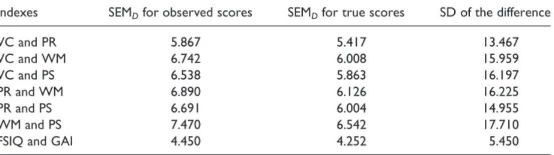
Table 8.Standard errors of measurement of the difference for observed scores and true scores, and standard deviations of the difference between short-form indexes (the equivalent statistics for comparison of short-form FSIQ and GAI are also included)

Indexes SEMDfor observed scores SEMDfor true scores SD of the difference

VC and PR 5.867 5.417 13.467 VC and WM 6.742 6.008 15.959 VC and PS 6.538 5.863 16.197 PR and WM 6.890 6.126 16.225 PR and PS 6.691 6.004 14.955 WM and PS 7.470 6.542 17.710

FSIQ and GAI 4.450 4.252 5.450

Table 9.Critical values (two-tailed) for determining the reliability of differences between short-form indexes using either observed scores or estimated true scores (the equivalent values for comparison of short-form FSIQ and GAI are also included)

Critical values forobservedscores

(pvalue) Critical values for estimated(pvalue) truescores

.15 .10 .05 .01 .15 .10 .05 .01 VC and PR 8.45 9.65 11.50 15.11 7.80 8.91 10.62 13.95 VC and WM 9.71 11.09 13.21 17.37 8.65 9.88 11.78 15.48 VC and PS 9.41 10.76 12.81 16.84 8.44 9.64 11.49 15.10 PR and WM 9.92 11.33 13.50 17.75 8.82 10.08 12.01 15.78 PR and PS 9.64 11.01 13.11 17.24 8.65 9.88 11.77 15.47 WM and PS 10.76 12.29 14.64 19.24 9.42 10.76 12.82 16.85

used to test if this difference is reliable. The formula for this latter standard error is: SEMDt ¼ ffiffiffiffiffiffiffiffiffiffiffiffiffiffiffiffiffiffiffiffiffiffiffiffiffiffiffiffiffiffiffi SEM2 XtþSEM2Yt q : ð7Þ

These standard errors are reported in Table 8 and critical values for the difference between estimated true Index scores are presented in Table 9. Just as is the case for differences between obtained scores, an alternative is to divide the difference between estimated true scores by the relevant SEMDtand calculate a probability for thezthereby

obtained (this is the method used by the computer programme that accompanies this paper).

Bonferroni correction when testing for reliable differences between index scores

Multiple comparisons are usually involved when testing if there are reliable differences between a child’s index scores (as noted, there are six possible pairwise comparisons). Thus, if all comparisons are made, there will be a marked inflation of the Type I error rate. Although neuropsychologists will often have ana priorihypothesis concerning a difference between two or more particular Index scores, it is also the case that often there is insufficient prior information to form firm hypotheses. Moreover, should a psychologist wish to attend to a large, unexpected, difference in a client’s profile then, for all intents and purposes, they should be considered to have made all possible comparisons.

One possible solution to the multiple comparison problem is to apply a standard Bonferroni correction to thepvalues. That is, if the family wise (i.e. overall) Type I error rate (a) is set at 0.05 then the pvalue obtained for an individual pairwise difference between two indexes would have to be less than 0.05/6 is to be considered significant at the specified value of alpha. This, however, is a conservative approach that will lead to many genuine differences being missed.

A better option is to apply asequentialBonferroni correction (Larzelere & Mulaik, 1977). The first stage of this correction is identical to a standard Bonferroni correction. Thereafter, any of thekpairwise comparisons that were significant are set aside and the procedure is repeated with k2l in the denominator rather than k, where l is the number of comparisons recorded as significant at any previous stage. The process is stopped when none of the remaining comparisons achieve significance. This method is less conservative than a standard Bonferroni correction but ensures that the overall Type I error rate is maintained at, or below, the specified rate.

This sequential procedure can easily be performed by hand but, for convenience, the computer programme that accompanies this paper offers a sequential Bonferroni correction as an option. Note that, when this option is selected, the programme does not produce exact p values but simply records whether the discrepancies between indexes are significant at the .05 level after correction.

Abnormality of differences between indexes

When attempting to detect acquired impairments, it is important to quantify the degree of abnormality (the rarity) of any differences in a child’s index score profile (that is, it is important to now what percentage of the normative population are expected to exhibit larger differences). In order to estimate the abnormality of a difference between index scores it is necessary to calculate the standard deviation of the difference between each

pair of indexes. When, as in the present case, the measures being compared have a common standard deviation, the formula for the standard deviation of the difference is: SDD¼spffiffiffiffiffiffiffiffiffiffiffiffiffiffiffiffiffiffiffi222rXY; ð8Þ wheresis the common standard deviation (i.e. 15 in the present case) andrXYis the

correlation between the two measures1_.

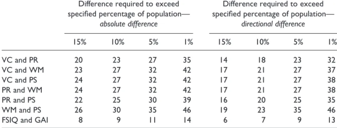
The standard deviations of the difference for the six pairings of index scores are presented in Table 8. To calculate the size of difference between index scores required for a specified level of abnormality the standard deviation of the difference for each pair of indexes was multiplied by values of z (standard normal deviates). The differences required to exceed the differences exhibited by various percentages of the normative population are presented in Table 10. Two sets of percentages are listed—the first column records the size of difference required regardless of sign, the second column records difference required for a directional difference. To illustrate, suppose a child obtains scores of 116 and 91 on the VC and PR indexes, respectively; the difference between the Index scores is therefore 25 points. Ignoring the sign of the difference, it can be seen from Table 10 that this difference is larger than that required (23) to exceed all but 10% of the population but is not large enough to exceed all but 5% of the population (difference required¼27 points). If the concern is with the percentage of the population expected to exhibit a differencein favourof VC, it can be seen that this difference is larger than that required (23) to exceed all but 5% of the population but is not large enough to exceed all but 1% (difference required¼32 points).

A closely related alternative to the approach outlined to is to divide an observed difference by the standard deviation of the difference and refer the resultantz(zD) to a

table of areas under the normal curve (or algorithmic equivalent) to obtain a precise estimate of the percentage of the population expected to exhibit this large a difference. To continue with the current example, it is estimated that 6.77% of the population would exhibit a difference of 25 points between VC and PR regardless of the sign of the difference and that 3.39% would exhibit a difference of 25 points in favour of VC. This latter approach is that used in the computer programme that accompanies the present paper (as was the case for reliable differences, these data are not presented in the present paper because they would require voluminous tables).

The methods used here to estimate the abnormality of differences between Index scores assumes that each pair of indexes follows a bivariate normal distribution. This statistical approach differs from the empirical approach used to estimate the abnormality of differences between indexes for the full-length WISC-IV. In the latter case the abnormality of differences are estimated by referring to a table (Table B.2) of the base-rates of differences observed in the WISC-IV standardization sample.

The aim with either approach is to estimate the percentage of the normative

populationthat will exhibit a larger difference than that observed for the case in hand and thusbothmethods provide onlyestimatesof the true abnormality of the difference. The developers of the WISC-IV preferred to base estimates of abnormality on directly observed differences in the standardization sample. On the other hand, the base-rate

1_{Note that this is an asymptotic method. That is, it does not consider the uncertainties involved in estimating the population}

mean andSDfrom normative sample data. Given the large size of the WISC-IV standardization sample its use is justifiable here. See Crawford and Garthwaite (2005) or Crawford and Garthwaite (2007) for a discussion of these issues and for optimal methods for normative samples with more modest Ns.

data will reflect any (presumably minor) departures from normality (i.e. ‘bumps and wiggles’) in the distribution of differences in the standardization sample, whereas the statistical approach will smooth these out.

A further difference between the two methods is that the estimates of abnormality provided by the statistical approach assumes that the integer-valued index scores represent underlying, smoothly continuous, real-valued scores, whereas the empirical approach does not make this assumption (in passing, note that a correction for continuity could be applied even when using the empirical approach). Opinions are liable to differ on whether the index scores should be treated as discrete or continuous. We favour the latter position, not least because most of the psychometric methods used with the WISC-IV make exactly this assumption (indeed the assumption of an underlying real-valued score is ubiquitous) and it is therefore consistent to apply it to the present problem; see Crawford, Garthwaite, and Slick (2009) for a recent, more detailed, discussion of the pros and cons of this assumption in psychological measurement in general.

One limitation of the statistical approach is that, at present, it estimates the rarity of Index score differences for the normative population as a whole, whereas with the empirical approach it is possible to examine the abnormality of these differences at different IQ levels. When this is done (see the WISC-IV technical and interpretive manual) it reveals that index score differences are typically smaller at low levels of IQ and that index score differences are not necessarily symmetric at a given level of IQ.

As a reviewer of this paper suggested, it is important to set out the differences between the statistical and empirical approaches. However, such a discussion should not detract from the fact that, for the present problem (i.e. estimating the abnormality differences in the normative population as a whole), one would expect the results obtained from the two approaches to exhibit a good degree of convergence. That is, because (a) the WISC-IV standardization sample is large, and (b) the standardization process should produce a multivariate normal distribution for the indexes, the differences between the two approaches will be relatively minor (indeed, were the differences marked, this would indicate that the indexes are not multivariate normal and would call into question many of the other statistical procedures used to interpret the full-length version).

Table 10. Difference between short-form indexes required to exceed various percentage of the normative population (the equivalent statistics for comparison of short-form FSIQ and GAI are also included)

Difference required to exceed specified percentage of population—

absolute difference

Difference required to exceed specified percentage of population—

directional difference 15% 10% 5% 1% 15% 10% 5% 1% VC and PR 20 23 27 35 14 18 23 32 VC and WM 23 27 32 42 17 21 27 37 VC and PS 24 27 32 42 17 21 27 38 PR and WM 24 27 32 42 17 21 27 38 PR and PS 22 25 30 39 16 20 25 35 WM and PS 26 30 35 46 19 23 35 46

Percentage of the population expected to exhibit j or more abnormally low index scores and j or more abnormally large index score differences

Information on the rarity or abnormality of test scores (or test score differences) is fundamental in interpreting the results of a cognitive assessment (Crawford, 2004; Strauss, Sherman, & Spreen, 2006). When attention is limited to a single test, this information is immediately available; if an abnormally low score is defined as one that falls below the 5th percentile then, by definition, 5% of the population is expected to obtain a score that is lower (in the case of Wechsler indexes, scores of 75 or lower are below the 5th percentile). However, the WISC-IV has four indexes and thus it would be useful to estimate what percentage of the normative population would be expected to exhibit at least one abnormally low Index score. This percentage will be higher than for any single Index and knowledge of it is liable to guard against over inference; that is, concluding impairment is present on the basis of one ‘abnormally’ low Index score if such a result is not at all uncommon in the general population. It is also useful to know what percentage of the population would be expected to obtain two or more, or three or more abnormally low scores; in general, it is important to know what percentage of the population would be expected to exhibitjor more abnormally low scores.

One approach to this issue would be to tabulate the percentages of the WISC-IV standardization sample exhibiting j or more abnormal index scores. However, such empirical base-rate data have not been provided for the full-length WISC-IV indexes, far less for short-forms. Crawford et al. (2007) have developed a generic Monte Carlo method to tackle problems of this type and have applied it to full-length WISC-IV Index scores. That is, they produced estimates of the percentage of the population expected to exhibitjor more abnormally low Index scores for a variety of different definitions of abnormality. We used this method (which requires the matrix of correlations between the short-form Index scores) to generate equivalent base-rate data for the present WISC-IV short-form: three alternative definitions of what constitutes an abnormally low score were employed: a score below the 15th, 10th or 5th percentile. The results are presented in Table 11a. If an abnormally low index score is defined as a score falling below the 5th percentile (this is our preferred criterion and hence appears in italic) it can be seen that it will not be uncommon for children to exhibit one or more abnormally low scores from among their four index scores (the base-rate is estimated at 14.9% of the population); relatively few however are expected to exhibit two or more abnormally low scores (3.92%), and three or more abnormally low scores will be rare.

A similar issue arises when the interest is in the abnormality of pairwise differences between indexes; i.e. if an abnormally large difference between a pair of indexes is defined as, say, a difference exhibited by less than 5% of the population, then what percentage of the population would be expected to exhibit one or more of such differences from among the six possible pairwise comparisons? The base-rates for this problem can also be obtained using Crawfordet al.’s (2007) Monte Carlo method and are presented in Table 11b. To make use of these data users should select their preferred definition of abnormality, note how many index scores and/or index score differences are exhibited by their case and refer to Table 11 to establish the base-rate for the occurrence of these numbers of abnormally low scores and abnormally large score differences. The computer programme accompanying this paper makes light work of this process: the user need only select a criterion for abnormality. The programme then provides the number of abnormally low scores and abnormally large differences exhibited by the case, along with the percentages of the general population expected to exhibit these numbers.

A global measure of the abnormality of a child’s index score profile

Although not available for the full-length version of the WISC-IV, it would be useful to have a single measure of the overall abnormality of a child’s profile of scores; i.e. a multivariate index that quantifies how unusual a particular combination of index scores is. One such measure was proposed by Huba (1985) based on the Mahalanobis distance statistic. Huba’s Mahalanobis distance index (MDI) for the abnormality of a case’s profile of scores onktests is:

x0_W21_{x; ð9Þ}

wherexis a vector ofz scores for the case on each of thektests of a battery andW21_is

the inverse of the correlation matrix for the battery’s standardization sample (the method requires the covariance matrix but the correlation matrix is the covariance matrix when scores are expressed asz scores). When this index is calculated for a child’s profile it is evaluated against a chi-squared distribution onk df. The probability obtained is an estimate of the proportion of the population that would exhibit a more unusual combination of scores.

This method has been used to examine the overall abnormality of an individual’s profile of subtest scores on the WAIS-R (Burgess, 1991; Crawford & Allan, 1994). However, it can equally be applied to an individual’s profile of Index scores; see Crawfordet al.(2008a) for its application to the profile of short-form index scores on the WAIS-III. Indeed, we consider this usage preferable given that research indicates that analysis at the level of Wechsler factors (i.e. indexes) achieves better differentiation

Table 11.Base rate data for the number of abnormally low index scores and abnormally large index score differences

(a) Percentage of the normative population expected to exhibit at leastjabnormally low Index scores on the short-form WISC-IV; three definitions of abnormality are used ranging from below the 15th percentile to below the 5th percentile

Criterion for abnormality

Percentage exhibitingjor more abnormally low WISC-IV short-form index scores

1 2 3 4

,15th 37.05 15.56 5.99 1.51

,10th 26.82 9.43 3.15 0.66

,5th 14.91 3.92 1.04 0.17

(b) Percentage of the normative population expected to exhibitjor more abnormal pairwise differences, regardless of sign, between short-form index scores on the WISC-IV; three definitions of abnormality are used ranging from a difference exhibited by less than 15% of the population to a difference exhibited by less than 5%

Percentage exhibitingjor more abnormal pairwise differences (regardless of sign) between WISC-IV short-form indexes

Criterion for abnormality 1 2 3 4 5 6

,15% 47.18 28.05 12.42 2.21 0.15 0.00

,10% 35.05 17.73 6.37 0.84 0.03 0.00

between healthy and impaired populations than analysis of subtest profiles (Crawford, Johnson, Mychalkiw, & Moore, 1997). The MDI was therefore implemented for the WISC-IV short-form: this index estimates the extent to which a child’s combination of index scores, i.e. the profile of relative strengths and weaknesses, is unusual (abnormal). Note that it is not a practical proposition to calculate the MDI by hand, nor is it all practical to provide tabled values as there is a huge range of possible combinations of index scores. Therefore, the MDI for a child’s profile of index scores is provided only by the computer programme that accompanies this paper.

A short-form GAI

The GAI for the WISC-IV is a relatively recent introduction. The full-length GAI is a composite formed by summing scores on the three VC and three PR subtests. That is, unlike the WISC-IV FSIQ, it does not include subtests from the WM or PS Indexes. It is assumed that psychologists who would make use of a short-form GAI are those who are already familiar with it and its potential applications in its full-length form.

A short-form GAI was formed using the sum of scaled scores on the Vocabulary, Similarities, Block Design, and Matrix Reasoning subtests. The psychometric methods employed to achieve this were those set out earlier for the four principal WISC-IV indexes and the FSIQ. The reliability of the short-form GAI was high (0.952;

SEM¼3:286) and only marginally lower than its full-length equivalent (the reliability of the full-length GAI calculated by the present authors was 0.958). The correlation between the short-form GAI and the full-length GAI was also very high (0.97).

A table (directly equivalent to that for the short-form FSIQ) for converting sums of scaled scores on the four GAI subtests to short-form GAI Index scores can be downloaded from http://www.abdn.ac.uk/,psy086/dept/GAI_Conversion_Table.htm (pressure of space prevents its inclusion in the present paper). Calculation of a short-form GAI is also included as an option in the computer programme that accompanies this paper. The main supplementary information available for interpretation of the full-length GAI consists of tables allowing users to examine whether (a) individuals’ GAI scores are reliably different from their FSIQ scores, and (b) whether these differences are abnormal. (See Tables F.2 and F.3 of the WISC-IV technical and interpretive manual). Equivalent information for the short-form GAI is presented in Table 9 (reliability of differences) and Table 10 (abnormality of differences) of the present paper.

Should index scores always be interpreted?

Flanagan and Kaufman (2004) have advised that, when there are large discrepancies between scores on the subtests contributing to an index, the index should not interpreted. Thus they suggest that an index should not be used when the difference between any of the subtests contributing to it exceeds five scaled score points. Opinions are liable to be divided on the merits of this advice. Daniel (2007), for example, has demonstrated using simulation studies that the construct validity of a composite ability measures was maintained in the face of a high degree of scatter among components contributing to it. We currently do not apply the Flanagan and Kaufman (2004) rule in our own practice but it is desirable that other psychologists should (a) be aware of its existence, and (b) be alerted when an individual’s scores violate it. The computer programme that accompanies this paper does not prevent the calculation of index

scores when subtest differences exceed five scaled score points but does issue a warning when this occurs.

A computer programme for scoring and analysing the index-based short-form

As noted, a computer programme for PCs (SF_WISC4.EXE) accompanies this paper. The programme implements all the procedures described in earlier sections. Although the paper contains all the necessary information to score and interpret a child’s short-form index scores (with the exception of the MDI and the provision of percentile limits for the effects of measurement error), the programme provides a very convenient alternative for busy neuropsychologists as it performs all the transformations and calculations (it requires only entry of the scaled scores on the subtests). The computer programme has the additional advantage that it will markedly reduce the likelihood of clerical error. Research shows that neuropsychologists make many more simple clerical errors than we like to imagine (e.g. see Faust, 1998; Sherrets, Gard, & Langner, 1979; Sullivan, 2000).

The programme prompts for the scores on the seven subtests used in the short-form and allows the user to select analysis options. There is also an optional field for entry of user notes (e.g. date of testing, an ID for the child etc) for future reference.

The output first reproduces the subtest scores used to obtain the short-form Index scores, the analysis options selected, and user notes, if entered. Thereafter it reports the short-form index scores with accompanying confidence limits and the scores expressed as percentiles (plus percentile confidence limits). It also reports the same results for the short-form FSIQ, and the short-form GAI, if the former has been requested. This output is followed by the results from the analysis of the reliability and abnormality of differences between the child’s index scores (including the base-rates for the number of abnormal scores and score differences and the MDI of the abnormality of the index score profile as covered in the two preceding sections). If the default options are not overridden the programme generates 95% confidence limits on obtained scores, and tests for a reliable difference between observed scores without applying a Bonferroni correction. When the option to calculate a short-form GAI has been selected, the output includes analysis of the reliability and abnormality of differences between the child’s GAI and FSIQ.

All results can be viewed on screen, edited, printed, or saved as a text file. A compiled version of the programme can be downloaded (as an executable file or as a zip file) from the following website address: www.abdn.ac.uk/,psy086/dept/sf_wisc4.htm.

Discussion

To illustrate the use of the foregoing methods and the accompanying computer programme, suppose that a child (of high premorbid ability) who has suffered a traumatic brain injury obtains the following scaled scores on the seven subtests that comprise the short-form: Vocabulary¼13, Similarities¼12, Block Design¼12, Matrix Reasoning¼12, Digit Span¼6, Coding¼4, and Symbol Search¼5. Suppose also that the psychologist requests calculation of the GAI, opts for 95% confidence limits (obtained using the traditional method) on obtained Index scores, chooses to examine the reliability of differences between observed (rather than estimated true index scores), opts not to apply a Bonferroni correction (as would be appropriate if they had

a priorihypotheses concerning the pattern of strengths and weaknesses), and chooses to define an abnormally low index score (and abnormally large difference between index scores) as a difference exhibited by less than 5% of the normative population (these are the default options for the computer programme).

The short-form index scores, accompanying confidence limits and percentiles for this case, obtained either by using Tables 2–7 or the computer programme, are presented in Figure 1a (the results for FSIQ and the GAI are presented also). This figure presents the results much as they appear in the output of the accompanying computer programme. Note that, in addition to the 95% limits on obtained scores, confidence

limits are also expressed as percentile ranks. Examination of the index scores reveals that the child’s index score on PS is abnormally low (it is at the 2nd percentile) and that WM is also relatively low (the score is at the 9th percentile). It can be seen from Figure 1b that these two indexes are significantly (i.e. reliably) poorer than the child’s scores on both the VC and PR indexes. Thus, in this case, it is very unlikely that the differences between these indexes are solely the result of measurement error; that is, there are genuine strengths and weaknesses in the child’s profile.

This pattern is consistent with the effects of a severe head injury in a child of high premorbid ability (Anderson, Northam, Hendy, & Wrennall, 2001; Rourke, Fisk, & Strang, 1986). However, low scores and reliable differences on their own are insufficient grounds for inferring the presence ofacquiredimpairments (Crawford & Garthwaite, 2005): a child of modest premorbid ability might be expected to obtain abnormally low scores, and many healthy children will exhibit reliable differences between their index scores. Therefore, it is also important to examine the abnormality of any differences in the child’s index score profile. In this case it can be seen from Figure 1c that the differences between the child’s PS and WM index scores and VC and PR scores are abnormal: that is, it is estimated that few children in the general population would exhibit differences of this magnitude.

It can also be seen from Figure 1c that, applying the criterion that a difference (regardless of sign) exhibited by less than 5% of the population is abnormal, three of the child’s differences are abnormal (i.e. VC vs. PS, VC vs. WM, and PR vs. PS). Application of Crawford et al.’s (2007) Monte Carlo method reveals that few children in the normative population are expected to exhibit this number of abnormal differences (2.00%). Moreover, the MDI, which provides a global measure of the abnormality of the child’s index score profile, is highly significant (x2_{¼13:059,p¼:01099). That is, the}

child’s overall profile is highly unusual. The results of analysing this child’s scores converge to provide convincing evidence of marked acquired impairments in PS and WM consistent with a severe head injury. The information obtained from an analysis such as this should then be combined with evidence from other testing, the history, and from clinical observation to arrive at a formulation of the child’s cognitive strengths and weaknesses and to draw out its implications for everyday functioning.

As the inputs for this example (i.e. the subtest scores) and outputs (Figure 1) are all provided, it may be useful for psychologists to work through this example (using either the tables or the accompanying programme) prior to using the short-form with their own cases.

Finally, note that the WISC-IV (an ability measure) can be used in tandem with an achievement measure, the Wechsler individual achievement test second edition (WIAT-II; Wechsler, 2002). The WISC-IV technical and interpretive manual (Wechsler, 2003b) presents a series of tables that allow a clinician to determine if differences between the five WIAT-II composite measures (Reading, Mathematics, Written Language, Oral Language, and Total Achievement) and WISC-IV FSIQ are (a) reliable and (b) abnormal. We suggest that these tables can also be used with the present WISC-IV short-form. The reliability of differences between the WISC-IV and WIAT-II composites is a function of the reliability of the two tests involved. The reliability of the short-form FSIQ (0.96) is almost indistinguishable from the reliability of the full-length FSIQ (0.97) and so it follows that the standard errors of the difference between the short-form FSIQ and the WIAT-II composites are also virtually indistinguishable from their full-length counterparts. Thus the existing tables of critical values can safely be used with the short-form FSIQ (the same applies to comparisons involving the short-form GAI).

Similarly, the abnormality of differences between the WISC-IV FSIQ and any WIAT-II composites is a function of the correlation between the two tests. As the correlation between full-length FSIQ and short-form FSIQ was very close to unity (0.99) it follows that the correlation between the WIAT-II composites and short-form FSIQ will be virtually identical to the correlations between the WIAT-II composites and full-length FSIQ. Thus again the existing table in the WISC-IV technical and interpretive manual (Table B.11) can be used with the short-form FSIQ.

In conclusion, we believe the WISC-IV short-form developed in the present paper has a number of positive features: it yields short-form index scores (rather than just a full scale IQ), it has good psychometric properties (i.e. high reliabilities and high validity), and offers the same useful methods of analysis as those available for the full-length version. The provision of an accompanying computer programme means that (a) the short-form can be scored and analysed very rapidly, and (b) the risk of clerical error is minimized. Some clinicians or researchers will no doubt take issue with the particular subtests selected for the WISC-IV short-form. As the methods used to form, evaluate, score and analyse the short-form are stated explicitly this should allow others to develop alternative short-forms based on the same approach.

References

Anderson, V., Northam, E., Hendy, J., & Wrennall, J. (2001). Pediatric neuropsychology: A clinical approach. London: Psychology Press.

Atkinson, L. (1991). Some tables for statistically based interpretation of WAIS-R factor scores.

Psychological Assessment,3, 288–291.

Burgess, A. (1991). Profile analysis of the Wechsler intelligence scales: A new index of subtest scatter.British Journal of Clinical Psychology,30, 257–263.

Charter, R. A., & Feldt, L. S. (2001). Confidence intervals for true scores: Is there a correct approach?Journal of Psychoeducational Assessment,19, 350–364.

Crawford, J. R. (2004). Psychometric foundations of neuropsychological assessment. In L. H. Goldstein & J. E. McNeil (Eds.),Clinical neuropsychology: A practical guide to assessment and management for clinicians(pp. 121–140). Chichester: Wiley.

Crawford, J. R., & Allan, K. M. (1994). The Mahalanobis distance index of WAIS-R subtest scatter: Psychometric properties in a healthy UK sample.British Journal of Clinical Psychology,33, 65–69.

Crawford, J. R., Allan, K. M., & Jack, A. M. (1992). Short-forms of the UK WAIS-R: Regression equations and their predictive accuracy in a general population sample.British Journal of Clinical Psychology,31, 191–202.

Crawford, J. R., Allum, S., & Kinion, J. E. (2008a). An Index based short form of the WAIS-III with accompanying analysis of reliability and abnormality of differences.British Journal of Clinical Psychology,47, 215–237. doi:10.1348/014466507X258859

Crawford, J. R., & Garthwaite, P. H. (2005). Testing for suspected impairments and dissociations in single-case studies in neuropsychology: Evaluation of alternatives using Monte Carlo simulations and revised tests for dissociations.Neuropsychology,19, 318–331.

Crawford, J. R., & Garthwaite, P. H. (2007). Comparison of a single case to a control or normative sample in neuropsychology: Development of a Bayesian approach.Cognitive Neuropsychol-ogy,24, 343–372.

Crawford, J. R., & Garthwaite, P. H. (2009). Percentiles please: The case for expressing neuropsychological test scores and accompanying confidence limits as percentile ranks.The Clinical Neuropsychologist,23, 193–204.

Crawford, J. R., Garthwaite, P. H., & Gault, C. B. (2007). Estimating the percentage of the population with abnormally low scores (or abnormally large score differences) on

standardized neuropsychological test batteries: A generic method with applications.

Neuropsychology,21, 419–430.

Crawford, J. R., Garthwaite, P. H., & Slick, D. J. (2009). On percentile norms in neuropsychology: Proposed reporting standards and methods for quantifying the uncertainty over the percentile ranks of test scores.The Clinical Neuropsychologist,23, 1173–1195.

Crawford, J. R., Henry, J. D., Ward, A. L., & Blake, J. (2006). The prospective and retrospective memory questionnaire (PRMQ): Latent structure, normative data and discrepancy analysis for proxy-ratings. British Journal of Clinical Psychology, 45, 83–104. doi:10.1348/ 014466505X28748

Crawford, J. R., Johnson, D. A., Mychalkiw, B., & Moore, J. W. (1997). WAIS-R performance following closed head injury: A comparison of the clinical utility of summary IQs, factor scores and subtest scatter indices.The Clinical Neuropsychologist,11, 345–355.

Crawford, J. R., Sutherland, D., & Garthwaite, P. H. (2008b). On the reliability and standard errors of measurement of contrast measures from the D-KEFS. Journal of the International Neuropsychological Society,14, 1069–1073.

Daniel, M. H. (2007). ‘Scatter’ and the construct validity of FSIQ: Comment on Fiorelloet al.

(2007).Applied Neuropsychology,14, 291–295.

Faust, D. (1998). Forensic assessment.Comprehensive clinical psychology(Vol. 4, pp. 563–599). Assessment, Amsterdam: Elsevier.

Flanagan, D. P., & Kaufman, A. S. (2004).Essentials of WISC-IV assessment. Hoboken, NJ: Wiley. Glutting, J. J., Mcdermott, P. A., & Stanley, J. C. (1987). Resolving differences among methods of establishing confidence limits for test scores.Educational and Psychological Measurement,

47, 607–614.

Huba, G. J. (1985). How unusual is a profile of test scores? Journal of Psychoeducational Assessment,4, 321–325.

Larzelere, R. E., & Mulaik, S. A. (1977). Single-sample tests for many correlations.Psychological Bulletin,84, 557–569.

Reynolds, C. R., Willson, V. L., & Clark, P. L. (1983). A four-test short form of the WAIS-R for clinical screening.Clinical Neuropsychology,5, 111–116.

Rourke, B. P., Fisk, J. L., & Strang, J. D. (1986).Neuropsychological assessment of children: A treatment oriented approach. New York, NY: Guilford.

Satz, P., & Mogel, S. (1962). An abbreviation of the WAIS for clinical use. Journal of Clinical Psychology,18, 77–79.

Sherrets, F., Gard, G., & Langner, H. (1979). Frequency of clerical errors on WISC protocols.

Psychology in the Schools,16, 495–496.

Silverstein, A. B. (1989). Confidence intervals for test scores and significance tests for test score differences: A comparison of methods.Journal of Clinical Psychology,45, 828–832. Stanley, J. C. (1971). Reliability. In R. L. Thorndike (Ed.),Educational measurement(2nd ed.,

pp. 356–442). Washington, DC: American Council on Education.

Strauss, E., Sherman, E. M. S., & Spreen, O. (2006).A compendium of neuropsychological tests: Administration, norms and commentary(3rd ed.). New York, NY: Oxford University Press. Sullivan, K. (2000). Examiners’ errors on the Wechsler memory scale-revised. Psychological

Reports,87(1), 234–240.

Tellegen, A., & Briggs, P. F. (1967). Old wine in new skins: Grouping Wechsler subtests into new scales.Journal of Consulting and Clinical Psychology,31, 499–506.

Wechsler, D. (2002). Wechsler individual achievement test second edition ( WIAT-II). San Antonio, TX: The Psychological Corporation.

Wechsler, D. (2003a).Wechsler intelligence scale for children(4th ed.). San Antonio, TX: The Psychological Corporation.

Wechsler, D. (2003b). WISC-IV technical and interpretive manual. London: Harcourt Assessment.