Nonparametric Density Estimation on A Graph: Learning Framework, Fast
Approximation and Application in Image Segmentation
∗Zhiding Yu
Oscar C. Au
Ketan Tang
Chunjing Xu
†
Dept. of Electronic and Computer Engineering
Hong Kong University of Science and Technology
{zdyu, eeau, tkt}@ust.hk
†
Shenzhen Inst. of Advanced Technology
Chinese Academy of Sciences
Abstract
We present a novel framework for tree-structure embed-ded density estimation and its fast approximation for mode seeking. The proposed method could find diverse applica-tions in computer vision and feature space analysis. Given any undirected, connected and weighted graph, the density function is defined as a joint representation of the feature space and the distance domain on the graph’s spanning tree. Since the distance domain of a tree is a constrained one, mode seeking can not be directly achieved by tradi-tional mean shift in both domain. we address this problem by introducing node shifting with force competition and its fast approximation. Our work is closely related to the pre-vious literature of nonparametric methods. One shall see, however, that the new formulation of this problem can lead to many advantages and new characteristics in its applica-tion, as will be illustrated later in this paper.
1. Introduction
Nonparametric density estimation provides a versatile tool for feature space analysis such as clustering and local maxima detection. The rationale behind, as pointed out by Comaniciu et al., is that ”feature space can be regarded as the empirical probability density function (pdf) of the repre-sented parameter.” Finding local estimated density maxima (or mode seeking) results in the computational module of mean shiftv [1], an old pattern recognition technique. The robust nature of mean shift leads to wide applications in low level computer vision, including edge preserved smoothing, image segmentation and object tracking. Recent works tries to improve its performance by introducing asymmetric bi-ased kernels in specific tasks, or seeks to reduce its com-plexity with fast algorithms.
∗This work has been supported in part by the Research Grants Council
(RGC) of the Hong Kong Special Administrative Region, China. (GRF 610109) 0 20 40 60 80 100 120 140 160 180 200 −70 −60 −50 −40 −30 −20
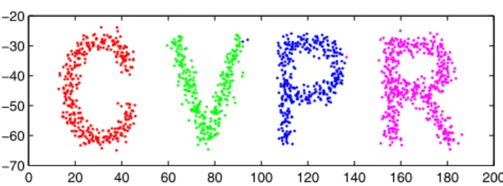
Figure 1. Example of data clustering using the proposed mode seeking algorithm withh1= 180andh2= 40.
We investigate the problem of tree-structure embedded density estimation, providing a novel angle looking into this problem. Our method introduces metrics learned from a spanning tree into mode seeking. In particular, we adopt minimum spanning tree (MST) to learn compact structures in the feature space or on a connected graph. On one hand, the inclusion of MST helps to find manifold structures for feature space analysis and data clustering. On the other hand, the graph-based attribute works compatibly with re-gional level image operations in computer vision. A wide range of computer vision problems in principle requires re-gional support, where relation between image regions are typically depicted with a weighted graph and graph-based methods have consequently become a powerful tool. Such characteristic offers several intuitionally reasonable advan-tages. First, region-wise operation allows one to investigate and design more versatile and powerful features, as a region often contains much more information than a single pixel. Second, adopting region as basic processing unit can largely alleviate the computational burden.
In the paper, we only illustrate the applications of our method in data clustering and region-based image segmen-tation, due to the limit of page length. Figure 1 shows one example of data clustering using our proposed method. The potential application of this algorithm, however, is consid-erable, as mode seeking has diverse applications.
This paper is organized as follows: In Section 2, we briefly introduce the background and closely related works.
Readers already familiar with nonparametric density esti-mation and mean shift may jump to Section 3, where we de-scribe the proposed method and discuss its important prop-erties. Some experimental results regarding clustering and application of our method in image segmentation are illus-trated in Section 4, showing that the method is an effective one. Finally, conclusions are made in the last Section.
2. Background and related works
Given a set of independent and identically distributed data points, nonparametric density estimation seeks to ap-proximate its pdf. Instead of representing the pdf by a sin-gle parametric model or a mixture model, the method finds a small number of nearest (or most similar) training instances and interpolate from them. To obtain smooth pdf estima-tion, gaussian kernel is commonly utilized as the kernel density estimator, also known as Parzen window.
The paradigm of density estimation and clustering in-cludes a family of mode seeking algorithms with Parzen density estimation. More recently, several works have ex-plored the improvement of traditional mean shift algorithm. In [2], the author introduced asymmetric kernel to mean shift object tracking. The scale and orientation of the kernel is automatically and adaptively selected, depending on the observations at each iteration. In [3], A new mode seeking algorithm called the medoid shift was proposed. The pur-pose of medoid shift is to extend mode seeking to general metric spaces. The method, however, requires huge compu-tational load and tends to result in over-fragmentation. It essentially becomes a finite point searching problem and is quite different from our method in terms of both pur-pose and algorithmic process. In [4], the authors propur-posed the quick shift algorithm which is considerably faster than mean shift and medoid shift. Their emphasis tends to con-centrate on algorithm acceleration while preserving its per-formance. The GPU implementation of quick shift was dis-cussed in [5] to further speed up the algorithm from the hardware perspective. There has also been other works try-ing to improve the efficiency of mode seektry-ing [8].
Considering the nearest neighbor property of MST, our method to some extent are related to previous works that generalize mean shift to non-linear manifolds [9], or intro-duce nonlinear kernelized or manifold metrics [3, 4]. Our method can achieve some similar goals but the idea remains very different. We also notice there exist a great many works concerning MST based graph segmentations [10]. Even though our method have also utilized MST, we gen-erally think it belongs to the family of mode seeking meth-ods where the algorithm characteristics are quite different from many graph based segmentation methods. Hence these methods may not fall within the scope of comparison in this paper. In fact our work presents a general framework of embedding tree structures into the mode seeking process.
Therefore it is straight forward for one to plug in many other trees and bring in additional algorithm characteristics.
3. Graph-based density estimation
We propose to perform density estimation on a joint do-main represented by the node feature space and the distance space defined by the minimum spanning tree of that graph. There are several advantages operating on an MST-based structure. First, tree-based structure helps to uniquely de-fine distances for any node pair, as a tree does not have circles. Of course, one could directly define the pairwise node distances in the Euclidean space, resulting in the tra-ditional mean shift. But this basically discards the struc-tural information preserved by a graph. In applications such as image segmentation, spatial information preserved by a graph can be very important. Second, an MST is the con-nected graph structure where all nodes are concon-nected with least edges numbers and weights. In other words, an MST can be regarded as a “compact” structure that preserves im-portant information about the cluster structure in a feature space. Although the introduction of a tree structure in prac-tice could possibly be problematic - as it faces the risk of large tree structure variation induced by noise points, es-pecially for those important tree roots - one shall see, the proposed method works pretty well and robustly in real im-age segmentation tests. In addition, such formulation helps to improve mode seeking performances for many manifold-shaped clusters.
There are several existing methods extracting an MST. In this paper, we adopt the Kruskal’s Algorithm to obtain the MST structure from the graph. We then define the den-sity function and describe its mode seeking process in the following part of this section.
3.1. Proposed density estimator
GivenN samples represented by the setV = {vi|i =
1, . . . , N,vi ∈ Rd} and the undirected weighted graph
G = (V,E), the minimum spanning tree S = (V,ES) is a connected graph of G withES⊆E,|ES|=N−1. For any node pair(i, j)wherei=j, there exists a unique path
Eij such thatEij ⊆ES,iandj is connected byEij and
deleting any element of the set results in the disconnection ofiandj. In addition, we defineEij to be∅, ifi=j.
Property 3.1 For any given node pair(i, j), the set of con-necting edgesEijis unique.
The above attribute comes directly from the tree structure. The proof is simple: if there is more than oneEijthen there exists at least one circle, which contradicts with the propo-sition. The unique distance definition on an MST facilitates the definition of density for a given location.
We propose to use a joint representation of the MST dis-tance space (or MST space for short) and the feature space
to define the density estimator. Consider the simplest case where the MST space kernel center is located exactly at a tree nodevj, then the density estimator can be written as
follows: f(v) =c0 i k d(vj,vi)2 h21 kv−vi h2 2, (1) whered(vj,vi) =
(vk1,vk2)∈Eij||vk1−vk2||is the cu-mulative weight of edges that connects the two nodes,vis the feature space kernel center,h1andh2are the bandwidth parameters controlling the window size andc0is a constant term determined by the sample size and bandwidth.k(x)is the profile of a normal kernel:
k(x) = exp(−1
2x). (2)
To define a density estimator for any location on the MST space, we have to first define the branch of an MST node. Here by saying “any location” we actually allow the MST space kernel center to be located on an MST edge be-tween neighboring nodes. In other words, the kernel can shift on the constrained space defined by MST. Suppose
vneigh is a neighboring node ofvi, we have the following
definition:
Definition 3.1 The branch of a given tree node vi with
respect to its connected edge (vi,vneigh) is a set of
nodes and edges B = (VB,EB), such that VB =
{vj|j = i,(vi,vneigh) ∈ Eij}, EB = {(vi,vj)|i =
j,(vi,vneigh)∈Eij}.
The branch of a node is an “induced subgraph” rooted atvi, and descending from its referenced connected edge.
There exist at least one corresponding MST edge - denoted aseref - where the MST space kernel center is located on.
If the center is located exactly on a tree node, then one may choose any edge connecting this node to one of its neighbor-ing nodes aseref. Suppose that the two nodes connected by
erefare respectivelyvref1andvref2, and that the distances
from the kernel center tovref1 andvref2are respectively
x1andx2(x1+x2=d(vref1−vref2) =||vref1−vref2||),
then the density estimator defined with respect tovref1can
be written as: ˆ feref,vref1(v, x1) = c0 i,vi∈Vref1 k (d(vref1,vi)−x1)2 h21 kv−vi h2 2+ c0 i,vi∈/Vref1 k (d(vref1,vi) +x1)2 h21 kv−vi h2 2. (3)
whereVref1is the set of branch nodes with respect tovref1
and eref. Similarly, we can define the density estimator
with respect tovref2:
ˆ feref,vref2(v, x2) = c0 i,vi∈Vref2 k (d(vref2,vi)−x2)2 h21 kv−vi h2 2+ c0 i,vi∈/Vref2 k (d(vref2,vi) +x2)2 h21 kv−vi h2 2. (4) whereVref2 is defined in a similar way. Associated with
the above density estimator are some good properties that facilitates the mode seeking process:
Property 3.2 fˆeref,vref1= ˆferef,vref2,∀eref ∈E
The above equality holds in the sense that Vref1 ∪
Vref2 = V and Vref1 ∩Vref2 = ∅, which indicates {vi|vi ∈ Vref1} = {vi|vi ∈/ Vref2}. In addition, since
d(vref1,vi)−x1=d(vref1,vref2)+d(vref2,vi)−x1=
d(vref2,vi) +x2whenvi ∈Vref1, we obtain the
follow-ing equality: i,vi∈Vref1 k (d(vref1,vi)−x1)2 h21 kv−vi h2 2 = i,vi∈/Vref2 k (d(vref2,vi) +x2)2 h21 kv−vi h2 2. The equality relation between the second term of (3) and the first term of (4) can be proved similarly. Property 3.2 states that the estimated density does not depend on the choice of reference point.
Property 3.3 If eref1 and eref2 are two edges that
connects the same node vref, fˆeref1,vref(v,0) =
ˆ
feref2,vref(v,0),∀vref ∈V.
Property 3.3 states that the estimated density does not de-pend on the choice of reference edge when the MST space kernel is located on a tree node. Here we consider the spe-cial situation where the MST space kernel is shifting from one edge to another. When the kernel is located onvref, the
density estimator degenerates to (1), asx = 0. The same condition also holds when we define the density estimator with respect to any other edge connecting tovref, which
indicates the above property.
Property 3.4 The kernel defined on the MST distance space is continuous and is piecewise differentiable.
According to the definition of density estimator, one is easy to verify the piecewise continuity and differentiability given the MST space kernel is located on the same edge. Together with Property 3.3, we can obtain Property 3.4. The above property also infers the continuity and piecewise differentiability of the density estimator since it is a linear combination of continuous and piecewise differentiable ker-nels.
3.2. Mode seeking with force competition
We seek the mode by maximizing the density estima-tor with respect to vandxsimultaneously. The step is to piecewisely estimate the density gradient, which is similar to mean shift. Taking the derivative of the density estimator with respect tov, one get the estimated density gradient:
∂fˆeref,vref(v, x) ∂v = 2c0 h22 i (vi−v)Kig v−vi h2 2 = 2c0 h22 i Kig v−vi h2 2 iKigv−h2vi 2v i iKigv−hvi 2 2 −v (5) whereg(x) =−k(x),Kiis the MST space kernel
func-tion: Ki=
k((d(vref,vi)−x)2/h21) ifvi∈Vref1
k((d(vref,vi) +x)2/h21) otherwise
The second term in (5) is the well known mean shift vec-tor for the feature space kernel centerv:
m(v) = iKigv−hvi 2 2v i iKigv−h2vi2 −v. (6) [1] has already developed a sound theoretical basis for mean shift algorithm concerning its physical meaning, conver-gence analysis and relation to other feature space anal-ysis methods. Here we will not extend the discussion. Now consider the second variable. Taking the derivative offˆeref,vref(v, x)with respect tox, we have:
∂fˆeref,vref(v, x) ∂x = 2c0 h21 i,vi∈Vref (d(vref,vi)−x)Kjoint,i +2c0 h21 i,vi∈/Vref (−d(vref,vi)−x)Kjoint,i, (7)
whereKjoint,iis the product of the feature space kernel and
the negative derivative of the MST space kernel profile:
Kjoint,i= ⎧ ⎨ ⎩ −k(d(vref,vi)−x)2 h21 kv−vi h2 2 ifvi∈Vref −k(d(vref,vi)+x)2 h21 kv−vi h2 2 otherwise Equation (7) can be further rewritten as:
∂fˆeref,vref(v, x) ∂x = 2c0 h21 i Kjoint,i i,vi∈Vref Kjoint,id(vref,vi) − i,vi∈/Vref Kjoint,id(vref,vi) / i Kjoint,i−x (8)
The last term of (8) results in the displacement of the MST space kernel, which is the so calledforce competition. Force competition can also be regarded as a special case of uni-variate mean shift withvref representing the origin. One
could imagine it as a tug of war where data points weighted byKjoint are tugging along each side ofvref. The
shift-ing step size, however, should be chosen carefully since ˆ
feref,vrefis only piecewise differentiable. Suppose we use
the msto denote the last term of (8), the displacement of the MST space kernel is defined as:
m(x) = max(−x,min(|eref| −x, ms)) (9)
The above term generantees that the MST space kernel is always shifted along the same reference edge. Here we seek to provide more intuition by discussing some properties of the density gradient estimation:
Property 3.5 The estimation of density gradient does not depend on the choice of reference nodevref.
Since the density estimator is piecewise differentiable on the edge, according to Property 3.2 we can verify the above property. The estimated density gradient, however, does de-pend on the choice of reference edge when the MST space kernel reaches a tree node with more than two connecting edges. Difference in the choice of the reference edge results in the following inequality:
Vvref,eref1∪Vvref,eref2=V,
whereVvref,eref1 is the branch node set with respect to
node vref and its connecting edge eref, and similar for
Vvref,eref2. Such inequality leads to the sudden jump of
estimated density gradient at some tree nodes.
Theorem 3.1 Given any nodevref where the MST space
kernel is located and there are more than two connecting edges, the number of reference edgeerefwith positive MST
Proof: Without loss of generality, suppose the MST space kernel is located on nodevref with three connecting edges
eref1,eref2anderef3, andDeref1 > Deref2 > Deref3,
whereDerefis defined as follows:
Deref = i,vi∈Vvref,eref −k d(vref,vi)2 h21 kv−vi h2 2d(vref,vi).
The force competition termmsvref,eref equals to the
esti-mated density gradient with respect tovref anderef times
a positive scalar: msvref,eref1=c ∂fˆeref,vref(v, x) ∂x x=0
=Dref1−Dref2−Dref3.
Similarly, we havemsvref,eref2 =Dref2−Dref1−Dref3
and msvref,eref3 = Dref3 − Dref1 −Dref2. Since
Deref1> Deref2 > Deref3andDeref >0,msvref,eref2
andmsvref,eref3 can not possibly be larger than 0. The
only positivemsvref,eref comes whenDref1 > Dref2+
Dref3and the above proof can be easily extended to nodes
with multiple edges. Thus we have proved the above Theo-rem.
3.3. Algorithmic description
Theorem 3.1 states that when the MST space kernel is located on any tree node, either this node is a local maxima, or there is only one edge to which shifting the kernel results in the increase of the density. The conveyed intuition here is important: each time the MST space kernel is shifting from one edge to another, one does not face the problem of multiple selectable paths since there is at most one edge that increases the estimated density. Such property leads to the basis of our implemented algorithm and its fast approx-imation method. The mode seeking algorithm is a step size controlled gradient ascent:
1. For each data point vi, i = 1,2, ..., N, initialize the
its feature space kernel position as the data point itself. Selectvi asvref and initialize the MST space kernel
on the reference node.
2. Compute the MST space kernel shift with the follow-ing rules:
If the MST space is exactly located on any tree node, calculatemj(x)|x=0 with respect to all its
con-necting edgesej.
If There exists one positivemj, select the
corre-sponding edgeejas the reference edgeeref.
m(x) =mjas the MST space kernel shift.
Else m(x) = 0.
Else calculatem(x)with respect tovref anderef.
3. Calculate the step control factorα: If m(x) = 0,α= 1.
Else α=|m(x)|/|ms|.
4. Compute the feature space kernel shift and scale it with α:m(v) =αm(v).
5. Simultaneously shift the MST space kernel and the feature space kernel with respect to the kernel shifts calculated in Step 2 and Step 4. The MST space kernel is shifted with the following rule:
If the MST space kernel is exactly located on a node If m(x) = |eref|, shift the MST space kernel
to the neighboring node connected byeref
and select the neighboring node as the new reference node.
Elseif m(x) = 0, the MST space kernel stays on the current node.
Else update the kernel position on the edge:x=
m(x).
Elseif the MST space kernel is located on an edge If m(x) ==−x, shift the MST space kernel to
the reference node.
Elseif m(x) = eref −x, shift the MST space
kernel to the neighboring node connected by eref and select the neighboring node as the
new reference node.
Else update the kernel position on the edge: x =
m(x) +x.
6. Repeat Step 2 to Step 5 until convergence.
3.4. Fast approximation
Due to the piecewise differentiability and step control, the above algorithm gives the best mode seeking perfor-mance but requires more iterations before convergence. In addition, the algorithm contains numerous ”if-then-else” conditions, which is not friendly to hardware implementa-tion. Here we also propose a fast approximation to the orig-inal algorithm by iteratively shifting the MST space kernel and the feature space kernel. The method is straight for-ward:
1. For each data point, initialize the MST space kernel and the feature space kernel.
3. If there exist neighboring nodes that increase the esti-mated density, shift the MST space kernel to the near-est one. Otherwise, stop shifting.
4. Repeat Step 2 and 3 until convergence.
In all of the following experiments, we only implement the above fast algorithm.
4. Experimental results
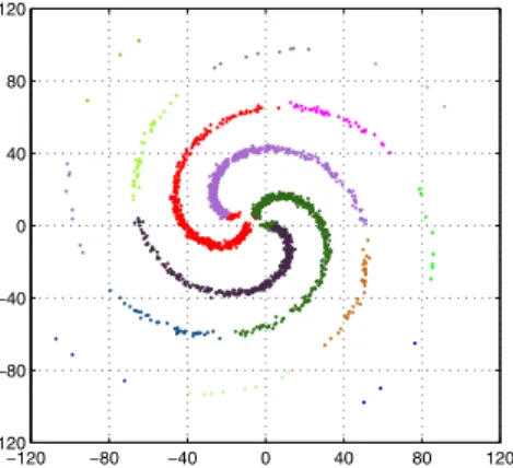
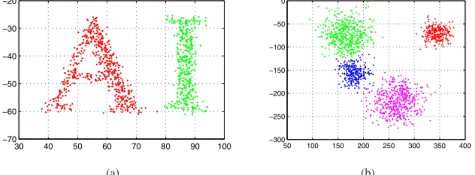
We show three sets of experiments using our proposed algorithm. The first set of experiments demonstrates the performance of the method in the task of data clustering. Figure 2(a) shows a character shaped distribution contain-ing 934 data points and its clustercontain-ing result. The bandwidth parametersh1 andh2were respectively set to 150 and 40 for this experiment. Figure 2(b) shows the mixture of 4 gaussian distributions with a total of 1500 data points. Here we seth1to 700 andh2to 150. From the two experiments one could observe that the method works reasonably well for both arbitrarily shaped and regularly shaped cluster of data. The real challenge comes when we want to cluster the spiral-like data distribution with highly nonlinear clus-ter separation boundaries. The example of spiral-like data given in [3] was reproduced with the Matlab code kindly available at http://www.cs.cmu.edu/∼new medoid.htm. In this experimenth1 andh2 are respectively set to 150 and 300. Note that we have achieved the clustering perfor-mance that approximates the one given in [3] without using any non-Euclidean metric, while mean shift or Euclidean medoid shift usually will fail on such task.
−120 −80 −40 0 40 80 120 −120 −80 −40 0 40 80 120
Figure 3. Clustering with spiral-like cluster of data using the pro-posed method
The second set of experiments address the problem dis-continuity preserved smoothing with superpixelized im-ages. As discussed in previous section, region-wise oper-ation significantly reduces the required computoper-ation power, thus greatly accelerates the image smoothing and segmen-tation process. The introduction of MST space kernel
works in compatible with the region adjacency graph and in addition, further improves the smoothing and segmen-tation performance. Figure 4 shows the images and their smoothing results using different methods in the RGB color space. The images are first superpixelized using normalized cut[6, 7]. The corresponding Matlab code is kindly pro-vided at http://www.cs.sfu.ca/∼mori/research/superpixels/. We set the number of coarse superpixelsN spto 200, the number of fine superpixelsN sp2 to 400 and the number of eigenvectorsN ev to 40. Each superpixel is then rep-resented by the mean RGB value and the whole image is mapped to an undirected, weighted region adjacency graph where edges corresponds to the eight-connectivities of two regions and edge weights are defined as the Euclidean dis-tances between the region means. We extract the mini-mum spanning tree from the region adjacency graph us-ing Kruskal’s Algorithm and perform mode seekus-ing usus-ing our proposed method. Here we fixed h1as 30 and h2 as 50 for all the test images. The obtained results are illus-trated in the second column of figure 4. To demonstrate the improvement of algorithm performance by introducing the MST space kernel, we compare the results with medoid shift smoothing where each super pixel is represented by the 5D joint representation of the RGB mean and spatial coordinate mean. The distance matrix is obtained by cal-culating the Euclidean distances between each pair of super pixels and the parameter Sigmais set to 2000. We also compare our results with quick shift which is a fast mode seeking algorithm. We run the quick shift algorithm with the VLFeat Matlab package which is publicly available at http://www.vlfeat.org/. The parametersratio,kernelsize andmaxdistare respectively set to 0.3, 12 and 30. The re-sults illustrated in figure 4 indicates the advantage of using our proposed method for image smoothing.
We illustrate the potential application of image segmen-tation using our method in the last set of experiments. Note that the segmentation performance depends largely on the defined feature. With superpixelized images, the definition of image feature becomes much more versatile than pixel based methods. Such framework allows one to improve the segmentation performance by defining the feature in a so-phisticated way, using textons, texture detectors or other re-gion statistics. For simplicity we only adopt rere-gion color histogram in this paper. Each region is represented by a 24-D concatenated histogram with each RGB channel re-turning a histogram of 8 bins. We then use principal compo-nent analysis (PCA) to perform dimensionality reduction on the obtained histograms. The percentage of preserved vari-ance for PCA is set to 0.9, a typical rule of thumb value for PCA. For most of the images, the reduced dimension after performing PCA often lies in between 4-8, which is much smaller than the original dimension number. By running PCA we reduces the computational complexity and
effec-30 40 50 60 70 80 90 100 −70 −60 −50 −40 −30 −20 (a) 50 100 150 200 250 300 350 400 −300 −250 −200 −150 −100 −50 0 (b)
Figure 2. Data clustering using the proposed method. (a) Clustering with linearly separable data. (b) Clustering with mixture of gaussians
Figure 4. Discontinuity preserved smoothing with superpixelized images: The first column contains the original images. The second column corresponds to the smoothing results using the proposed method. The second column contains the smoothing results using medoid shift. The last column are the results obtained by quick shift.
tively avoids from suffering the ”curse of dimensionality”. The segmentation results are shown in figure 5. One could observe that the proposed method is effective and produces reasonably good segmentations.
5. Conclusion
In this paper, by introducing the MST space kernel, we have proposed a novel mode seeking method that can im-prove mode seeking performance on manifold-structured data and can work compatibly with region-wise image
pro-Figure 5. Image segmentation experiments with region histogram
cesing operations. We achieved good algorithm perfor-mance in clustering data with highly nonlinear separation boundaries without using any manifold distance or some other non Euclidean metrics, which is of considerable chal-lenge. The advantage of using the proposed method for im-age smoothing and segmentation is also supported by our experiments.
References
[1] D. Comaniciu and P. Meer. “Mean shift: A robust ap-proach toward feature space analysis.” IEEE Trans. Pattern Anal. Mach. Intell., 24(5):603-619, 2002. [2] A. Yilmaz, “Object tracking by Asymmetric kernel
mean shift with automatic scale and orientation selec-tion.” InCVPR, 2007.
[3] Y. A. Sheikh, E. A. Khan and T. Kanade. “Mode-seeking by Medoidshifts.” InICCV, 2007.
[4] A. Vedaldi and S. Soatto. “Quick shift and kernel methods for mode seeking.” InECCV, 2008.
[5] A. Vedaldi and S. Soatto. “Really quick shift: Image segmentation on a GPU.” InWorkshop on Computer Vision using GPUs, held with ECCV, 2010.
[6] J. Shi and J. Malik. “Normalized cuts and image seg-mentation.”IEEE Trans. Pattern Anal. Mach. Intell., 22(8):888-905, 2000.
[7] X. Ren and J. Malik. “NLearning a classification model for segmentation.” InICCV, 2003.
[8] K. Zhang, J. T. Kwok and M. Tang. “Accelerated con-vergence using dynamic mean shift.” InECCV, 2006. [9] R. Subbarao and P. Meer. “Nonlinear mean shift for clustering over analytic manifolds.” InCVPR, 2006. [10] O. J. Morris, M.de J. Lee, and A.G. Constantinides.
“Graph theory for image analysis: An approach based on the shortest spanning tree,” InIEE Proc. F., Com-munications. Radar & Signal Processing, 133:146-152, 1986.