SCHEME BY THE ADVANCING FRONT METHOD
C. T. CHAN AND K. ANASTASIOU*Department of Civil Engineering, Imperial College of Science, Technology and Medicine, London, U.K.
SUMMARY
The paper deals with the discretization of any given multi-connected volume into a set of tetrahedral elements. A simple but robust tetrahedrization scheme based on a two-stage advancing front technique is presented. The method evolves from the triangulated domain bounding surfaces for which geometry representations are derived from triangular BeÄzier patches. Tetrahedral elements are then generated which ®ll the domain volume based on the set of distributed interior nodes. A new and ecient procedure is introduced for the distribution of the mesh interior nodes which uses an inverse-power interpolation technique. The proposed scheme is robust in that it is capable of tetrahedrizing a given arbitrary domain of any degree of irregularity, and allows the distribution of its interior nodes to be speci®ed by the user. Results are presented typical of those which might be encountered in hydrodynamics modelling involving ¯ows with a free surface.
Communications in Numerical Methods in Engineering, vol. 13, 33±46 (1997) (No. of Figures: 12 No. of Tables: 0 No. of Refs: 15)
KEY WORDS advancing front; tetrahedrization; inverse-power interpolation; triangular BeÄzier patches
1. INTRODUCTION
The task of decomposing a problem domain into a set of discrete elements, which is the ®rst step in the numerical solution of sets of partial dierential equations using ®nite element, ®nite dierence, or ®nite volume based methods, is by no means trivial. In many applications, the geometry of the problem domain is arbitrary in shape and has irregular bounding surfaces. In order to achieve an accurate representation of such domain geometries one often requires tens of thousands of discrete elements with straight sides. As a result, the availability of a robust and versatile automatic mesh generator has become a prerequisite in current numerical modelling eorts.
Numerous semiautomatic and automatic mesh generation techniques are available. A review of such techniques can be found in the papers by Thacker1 and Ho-Le.2 A discussion of the relative merits and shortcomings of the available methods for two- and three-dimensional problem domains has been presented by Lo.3The Delaunay triangulation technique,4±6the ®nite octree technique,4±6 and the advancing front technique3;10±11 are the most widely used tech-niques, and they are all well described in the literature. In the present work, the advancing front technique is selected in view of its relatively simple algorithm, its eectiveness in element shape control,3;10 and its proven track record in large scale computational modelling.10;11
CCC 1069±8299/97/010033±14 Received 26 October 1995
#1997 by John Wiley & Sons, Ltd. Revised 10 April 1996 * Author to whom correspondence should be addressed.
The motivating force for the work presented herein arises from a particular interest in the application of ®nite volume based analysis techniques to the modelling of hydrodynamics in coastal engineering problems. The problem domains encountered in such applications are typi®ed by a continuously varying geometry, with the domain bounding surfaces exhibiting a characteristically high degree of irregularity. The present work is therefore carried out with the objective to construct an ecient and robust tetrahedral mesh generator which is generally applicable and suciently versatile for modelling coastal ¯ows with a free surface.
The application of the tetrahedral mesh generation algorithm involves two distinct stages. They are:
1. triangulation of the domain bounding surfaces
2. tetrahedrization of the domain volume based on the triangulated bounding surfaces. A detailed discussion of the features and implementation of the ®rst stage of the algorithm has been presented by Anastasiou and Chan.13 This paper therefore focuses on the second stage, which deals with the domain tetrahedrization process. Section 3 of the paper is a brief review of the steps involved in triangulating the volume bounding surface, together with the ordering process required for the surface triangular meshes. In Section 4 the distribution of domain interior nodes by an inverse-power interpolation technique is discussed. Unlike the conventional methods whereby interior nodes are distributed on a speci®ed set of cutting planes of the problem domain, the present procedure distributes the interior nodes in 3D space in accordance with user speci®ed mesh density requirements. Finally, the domain tetrahedrization process is presented in Section 5, where also the performance of the algorithm is accessed and results are presented and discussed.
2. TRIANGULATION OF DOMAIN BOUNDING SURFACES AND ORDERING OF SURFACE MESHES
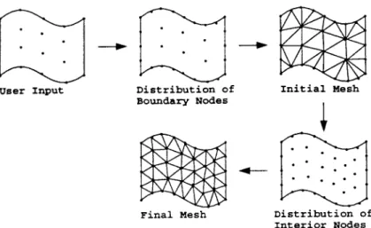
The ®rst stage of the volume tetrahedrization process using the advancing front method involves the triangulation of the domain bounding surfaces. The surface triangulation process entails the following steps:
1. distribution of boundary nodes along the boundaries of the surface domain
2. generation of an initial mesh based on the distributed boundary nodes, and user input interior nodes, if present
3. derivation of boundary geometry representation based on the generated triangular initial mesh. This is achieved using triangular BeÄzier patches withG1 continuity
4. distribution of interior nodes within the surface domain
5. generation of a triangular mesh on the surface domain by linking together the distributed interior nodes.
The distribution of boundary nodes and interior nodes in steps 1 and 4 is based on user speci®ed values of node spacing control parameters of an associated pre-established node
Figure 1. Generation of triangular mesh on domain bounding surfaces
spacing function. The advancing front technique is used in steps 2 and 5 for the triangular mesh generation. Figure 1 gives a schematic diagram of the surface mesh generation process. Local remeshing of the triangulated surface can be carried out, if desired, over regions speci®ed by the user. This is accomplished by carrying out steps 2, 4 and 5 locally over the speci®ed regions.
The ®rst stage of the overall tetrahedrization process is completed when all the bounding surfaces are duly triangulated. It is important to highlight that by following the above procedure for surface triangulation, before the triangulation process actually begins, a given domain closed surface is already segmented into subregions, each of which is projectable onto a plane. As a result of this surface decomposition, bounding surface triangulation is accomplished subregion-by-subregion with the connections between them carefully matched.
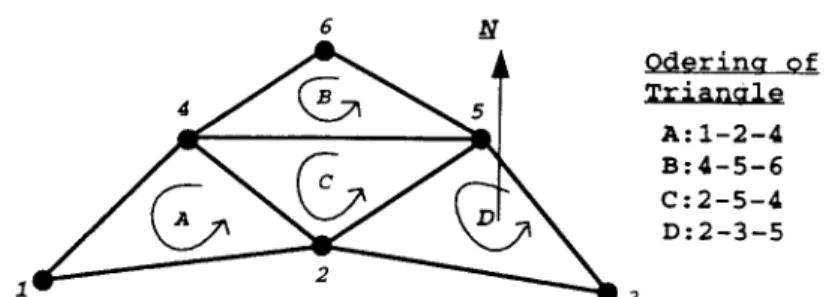
Although it is straightforward to decompose a given closed surface into a combination of projectable subregions and triangulate them independently, the resulting set of triangulated surfaces will possess triangular facets with incompatible order and numbering system when the subregions are combined. In order to carry out volume tetrahedrization by the advancing front method, the triangular facets must be consistently arranged and their normals properly identi-®ed. Following a similar procedure as outlined by Lo,14 the ordering of the triangular facets is accomplished in the following steps:
1. deletion of the duplicate lines of the triangular mesh. Duplication of lines occurs when two neighbouring triangulated subregions are merged
2. calculation of the element sizes of the triangular mesh in order to determine the node spacing distribution on the bounding surfaces. Node spacing information is used for the subsequent distribution of interior nodes
3. ordering of the triangular mesh. The triangular facets are ordered according to a consistent numbering system so that their normals always point outwards from the interior of the domain, as depicted in Figure 2.
3. DISTRIBUTION OF INTERIOR NODES
In order to discretize a given volume into a set of well conditioned tetrahedral elements with arbitrary gradation, a ¯exible procedure is adopted for the distribution of the interior nodes in
accordance with a speci®cation provided by the user. This is accomplished in the following steps:
1. the node spacing distribution on the domain bounding surfaces is established based on the calculated element sizes of the bounding surface meshes, as described earlier
2. `clustering nodes' are introduced into the domain volume at user speci®ed locations in order to control mesh density in their vicinity. Each such node is prescribed with node spacing control parameters, from which node spacing information is evaluated according to a user de®ned node spacing function. It is noted that the clustering nodes are `phantom nodes' and will not be included in the set of nodes of the ®nal generated mesh
3. at any location in the domain node spacing information is interpolated from the nodes on the domain bounding surface and the clustering nodes
4. an interior node is generated when, within the circumsphere de®ned by the node spacing function, no other mesh points are encountered
5 steps 3 and 4 are repeated at all locations in the domain and the distribution of interior nodes is terminated when the domain volume is completely interrogated.
It is worth highlighting that the information required in order for step 2 above to be carried out is input by the user and is necessary only when speci®c clustering or distribution of mesh points at arbitrary locations within the interior of a problem domain is required. The intro-duction of a clustering node requires the speci®cation of the coordinates of the clustering node xc;yc;zc, together with the corresponding set of values of the spacing control parameters
ftp1;tp2;. . .;tpng, which are used to evaluate the node spacing function. In general, the spacing
parameters and the associated node spacing function are problem dependent. In the context of modelling ¯ows with a free surface, for example, the spacing control parameters may be set equal tofC;g;h;tg, whereCis the Courant number,gis the gravitational acceleration,his the local water depth, which is a function of the clustering node coordinates, andtis the time step. In this case the associated node spacing function may be de®ned as the Courant number relationship given bylt= Cp gh.
The external limits of the problem domain, de®ning the embodying cuboid, must ®rst be established before the distribution of interior nodes is carried out. This cuboid is segmented into a collection of cubes with side dimension, which is de®ned as the `interrogation interval'. The corners of the cubes are correspondingly termed `interrogation points'. The generation of interior nodes is investigated at each of the interrogation points by carrying out steps 3 and 4 as de®ned above. The process of interior nodes generation is carried out plane by plane, sweeping through all the interrogation points, starting from the bottom plane of the cuboid and moving progressively upwards towards its top.
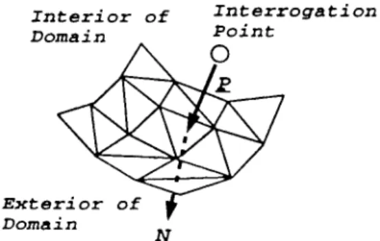
In order to avoid having interior nodes distributed outside the problem domain, an `entrance' test is carried out at each interrogation point, in order to invalidate any interrogation point that is located outside of the problem domain. This entrance test is accomplished by requiring that the dot product between the vectorsPandNis always less than zero (Figure 3), wherePis the vector from the interrogation point to the centroid of the nearest triangle facet on the domain surface, andNis the normal to the corresponding triangle facet as de®ned earlier in Section 3.
3.1. Inverse-power interpolation for node spacing information
An important process in the above procedure which requires more explanation is the inter-polation of node spacing information in step 3 above. In satisfying the requirement for ¯exibility and simplicity, the interpolation process is accomplished using the inverse-power interpolation technique as described below.
At a given interrogation point x;y;z in the domain volume, node spacing information is given as a function of the inverse power of the distance to each of the surrounding spacing information nodes (i.e. nodes prescribed with node spacing information). This is expressed as
f x;y;z Xn i1 f xi;yi;zi dm i .Xn i1 1 dm i
where f x;y;z is the node spacing function which provides the information dictating the tetrahedra edge length to be generated,diare the distances from the interrogation point x;y;z to the spacing information nodes xi;yi;zi,mis an integer specifying the power of interpolation andnis the number of points used in the interpolation. High values ofmwill result in sharper variation in node spacing distribution, and vice versa. In the present algorithm,mis set to 2 andn
is set to 4.
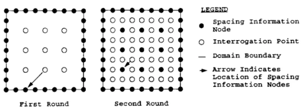
In order to achieve better eciency, the interpolation process is accomplished in two passes. In the ®rst pass a coarse interrogation interval is used and the interpolated node spacing information is stored at each of the interrogated points. Consequently, node spacing information is available at every interrogated interval of the volume domain. In the second pass the volume domain is interrogated with a ®ne interrogation interval and the interpolation of node spacing information is carried out `locally'. This is accomplished in view of the fact that at any given position in the domain its neighbourhood is already ®lled with node spacing information established during the ®rst pass. As a result of following this procedure the interpolation process is expedited and the distribution of interior nodes can be accomplished using as ®ne an
Figure 4. Distribution of interior nodes is done by two rounds of inverse-power interpolation process
interrogation interval as desirable without consuming excessive processing time. Figure 4 illustrates this process.
3.2. Location of neighbouring spacing information nodes
In order to ensure a good interpolation of node spacing information the current interrogation point should be surrounded `evenly' by spacing information nodes. For a four points inverse-power interpolation this requires the selected spacing information nodes to form a tetrahedron enclosing the interrogation point.
The location of the ®rst spacing information node is simply the nearest one to the inter-rogation point (Figure 5(a)). The second spacing information node is chosen so that an obtuse angle is formed between the ®rst selected node and the second one at the interrogation position (Figure 5(b)). This is achieved by selecting the second node as the nearest point to the inter-rogation point satisfying the relationship
r01r0240
wherer01andr02denote the vectors from the interrogation point to the selected ®rst and second nodes, respectively. The third spacing information node is chosen so that it is the closest one located within the region which lies between the back extension of the two planes each of which passes through the line formed either by the ®rst or the second selected nodes with the inter-rogation point and perpendicular to the plane formed by them (Figure 5(c)). This requires the satisfaction of the relationship
ja01a02a03j 41
wherea01;a02 anda03 denote the unit vectors from the interrogation position to the respective selected nodes. Finally, the fourth spacing information node is selected as the nearest node which, together with the three already selected nodes, form a tetrahedron enclosing the inter-rogation point (Figure 5(d)). In order to establish whether the interinter-rogation pointPis within the tetrahedronABCD, the volumesV1,V2,V3andV4must ®rst be computed, as follows:
V1PA PBPC V2PA PDPC V3PA PBPD V4PB PDPC
Figure 5(a). Location of ®rst spacing information
node Figure 5(b). Location of second spacing informationnode
Figure 5(c). Location of third spacing information
node Figure 5(d). Location of fourth spacing informationnode
PointPis within the tetrahedron when
min V1V2;V1V3;V1V4;V2V3;V2V4;V3V450
It should be noted that, when a given interrogation point lies on the plane formed by the ®rst three selected nodes of a tetrahedron, the selection of the fourth node is not straightforward owing to the uncertainty associated with determining the `enclosing tetrahedron'. This problem can be resolved by ®rst perturbing the interrogation point out of the plane on which it is attached before the selection of the fourth node is carried out. The perturbation has to be done twice in two opposite directions perpendicular to the plane, and the selection of the fourth node is carried out twice. In this case, the fourth node selected is the one associated with the smallest tetrahedron out of the two.
4. DOMAIN TETRAHEDRIZATION
Following the distribution of interior nodes, the advancing front technique is used to link the generated nodes so as to form tetrahedral elements. In a way similar to that adopted for the triangulation of the domain bounding surfaces, the generation of tetrahedral elements starts from the bounding surfaces and proceeds inwards. The generation process terminates when the whole of the domain volume is ®lled with tetrahedral elements. The initial generation front is composed from the set of triangular facets making up the domain bounding surfaces. A tetra-hedron element is generated when a triangular facet from the generation front successfully locates an additional node to form a tetrahedron. The generation front is updated whenever a new tetrahedron element is formed. As a result, the generation front changes continuously throughout the process of tetrahedrization.
Let be the set of nodes on the generation front andbe the set of interior nodes remaining inside the polyhedron formed by the generation front. The objective is to locate a nodePsuch
thatP2 [so that the resulting tetrahedron is completely located within the region enclosed by the generation front. This requirement can be satis®ed by allowing
C1C3C1C2C1P>0
whereC1;C2;C3are the vertices of a triangular facet on the generation front, and the order of the vertices is such that the normal vector to the triangular facet is pointing outward from the interior of the domain (Figure 6). In order to ensure that the potential tetrahedron does not cut across the generation front and does not enclose any existing tetrahedra, an extra check must be made so that no node from the setf [ÿ fC1;C2;C3;Pggis enclosed by it.
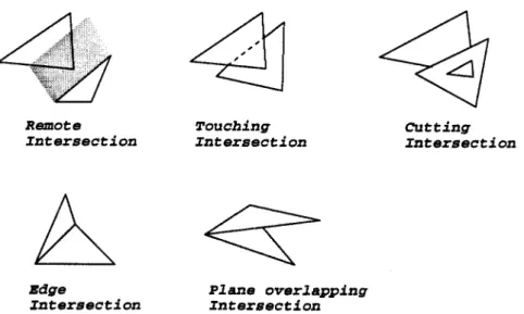
Two additional constraints must be satis®ed for a node to be chosen to form a new tetrahedron with a triangular facet. The ®rst is that the potential tetrahedron should not intersect with any of the existing tetrahedra, and the second is that it possesses an optimum tetrahedron shape factor. Detection of possible intersection between the facets of a potential tetrahedron and already formed tetrahedra is done by ®rst establishing whether the line of intersection between a pair of triangular facets cuts through the edges of the two facets. If this is the case then the two facets from the potential and already formed tetrahedra will be ¯agged for further examination, where one of the following four intersection cases would be identi®ed. These are the `remote' inter-section, the `touching' interinter-section, the `cutting' intersection and the `edge' intersection (Figure 7). If no intersection between two triangular facets is detected, the triangular facets will be ¯agged for further examination for `overlapping' intersection (Figure 7). Intersection between a potential and already formed tetrahedron is said to have occurred if one of the triangular facets of the potential tetrahedron has incurred either touching, cutting or overlapping intersection.
In order to optimize the tetrahedron shape, the radius shape factor as de®ned by Liu and Joe15 is used to control the potential node selection
03Rin=Rcirc
where Rin and Rcirc denote the in-sphere radius and circumsphere radius of a tetrahedron, respectively. For a regular tetrahedron, 0 assumes the maximum value of 1. Following a procedure similar to that adopted by Lo,3 future tetrahedron shape factors associated with the triangular facets of the potential tetrahedron are also considered during the selection of a potential node. Consequently, the determining tetrahedron shape factor is de®ned as
o123 Figure 6. Formation of tetrahedronC1C2C3P
where1,2and3are the future tetrahedron radius shape factors associated with the triangular facets of the potential tetrahedron. A potential node is actually selected when its associated
value is the maximum obtainable.
After the potential node selection, a new tetrahedron is formed and the generation front has to be updated. Referring to Figure 6, the four triangular facets of the tetrahedronC1C2C3Phave to be considered in turn, and the generation front can be updated by:
1. removing triangular facetC1C2C3 from the generation front
2. removing triangular facetC2C1Pfrom the generation front if it is part of it, addingPC1C2 to it otherwise
3. removing triangular facetC1C3Pfrom the generation front if it is part of it, addingPC3C1 to it otherwise
4. removing triangular facetC3C2Pfrom the generation front if it is part of it, addingPC2C3 to it otherwise.
Upon completion of the mesh generation process local mesh re®nement can be carried out on the generated tetrahedral mesh by an octree type cell division strategy, as proposed by Vijayan and Kallinderis.11 Essentially, an element ¯agged for re®nement is further divided into eight children through inserting mid-edge nodes into the element edges as shown in Figure 8(a). As a result of this process, hanging nodes are generated on some or all of the edges of the neigh-bouring tetrahedra abutting the divided elements. In order to eliminate these hanging nodes, the abutting tetrahedra are then divided using a directional division strategy. Three dierent cases for element directional division can be encountered. In the ®rst case where all the hanging nodes appear on the same face of the element, it is directionally divided into four children elements (Figure 8(b)). In the second case where only one hanging node appears on the element edges, the element is divided into two children elements as shown in Figure 8(c). Finally, when the hanging nodes do not produce the patterns of either one of the ®rst two cases, a centroidal node is introduced in the element, which is then divided into tetrahedral child elements by connecting the vertices of the element and the hanging nodes to the centroidal node (Figure 8(d)).
Following the completion of the tetrahedrization process, mesh smoothing is carried out. This is done using the standard Laplacian smoothing technique, whereby each of the interior nodes is
shifted to the centre of the surrounding polyhedron.3The iteration for smoothing is terminated when no further signi®cant improvement of the overall tetrahedra shape measure 1i=n is achievable.
Two examples of the tetrahedrization process based on the present scheme are illustrated in Figures 9(a)±9(d) and Figures 10(a)±10(c). It is noted that the generated tetrahedral elements are of high quality with element radius shape factors 076 and 078 respectively. These values are very similar to those reported by Lo3 where an average value of 073 of the mean shape factorwas obtained. It is worth highlighting that the radius shape factors should not be compared directly with the mean shape factor reported above as they are obtained from domains with dierent boundary surfaces. However, for a large class of tetrahedral with radius shape factorgreater than 05, the mean shape factorwill be correspondingly higher.15 As a result, it is concluded
Figure 8(a). Mesh re®nement by splitting an element
into eight child elements Figure 8(b). Element is directionally divided into fourchild elements
Figure 8(c). Element is directionally divided into two
child elements Figure 8(d). Element is split by introducing a centroidalnode. Figure showing three child elements produced by face `bcd'
that the present scheme is capable of discretizing highly irregular problem domains with very satisfactory results.
4.1 Assessment of tetrahedrization using the advancing front technique
It is well known that the main advantages of the advancing front method are its eectiveness in element shape control and the simplicity of the algorithm. Nevertheless, a robust advancing front
Figure 9(b). Example of triangulated lower bounding surface of a basin
Figure 9(c). Upper and lower bounding surfaces are combined to form a volume domain in 3D space
mesh generator should also be endowed with the capability to discretize any given domain regardless of the distribution of its interior nodes. However, it is noted from present experience that, unlike 2D triangulation, it is not formally certain that a given volume domain can be arbitratrily discretized into tetrahedra using the point-based two-stage advancing front method. In other words one may encounter `unclosurable gaps' during the process of tetrahedrization.
Figure 10(a). Example of triangulated bottom pro®le of a river system
Figure 10(b). A section through the tetrahedrized domain
This situation is particularly encountered in regions where the variation of node spacing distribution is acute. One example of such a problem is depicted in Figure 11(a), where the triangular facetsa;b;care trapped by triangular facetsd;e;f. Connections between points 1,2 and points 1,3 are blocked by triangular facetd and connection between points 1,4 is blocked by triangular facet e. Another example is illustrated by a cubicle gap with triangular facets as arranged in Figure 11(b). To overcome this problem, local mesh regeneration is required when-ever such 'unclosurable gaps' are detected.
Local mesh regeneration is achieved by ®rst `digging out' all the triangular facets aected by the unclosurable gap, leaving behind a cavity with size slightly larger than the gap. This process is done by de®ning a sphere with its centre located at the centroid of the gap and with radius of length reaching the most distant aected node. All triangular facets that are enclosed or intersected by this sphere are `dug out'. Local mesh regeneration is then carried out inside the cavity. This process may be accomplished in conjuction with local perturbation of the interior nodes within the cavity.
When the advancing front method is used for volume discretization, generation of slivers is not common as the tetrahedron shape factor is carefully accessed during each step of the mesh generation process. However, when the pattern of the interior nodes is arbitrary and far from uniform, the generation of slivers is usually unavoidable. In order to remove as many generated slivers as possible, one may either activate local mesh regeneration or adopt the conventional sliver removal strategies.
Conventionally, a sliver can be removed by using one of the following two strategies. For the case of the type (a) sliver shown in Figure 12, where two of the abutting tetrahedra share a common vertex, the sliver is removed by replacing the tetrahedraABDEandBCDEwithABCE
andACDE, respectively. For the cases of the type (b) sliver whereABDEandBCDE cannot be replaced by ACDE and ABCE, and the type (c) sliver where none of the sliver abutting
Figure 11(a). Triangular fronts `a,b,c' are trapped by
fronts `d,e,f' Figure 11(b). `Unclosurable problem' depicted by acubicle space
polyhedron volume.
5. CONCLUSIONS
In this paper a scheme for 3D volume tetrahedrization using the advancing front technique is presented. The method ®rst triangulates the bounding surfaces of the given problem domain, followed by the tetrahedrization of the domain volume. A simple but ecient algorithm is proposed for the distribution of interior nodes using the inverse-power interpolation technique. This technique allows distribution of mesh points in an arbitrary manner according to user speci®cation. The robustness of the scheme has been demonstrated by discretizing domains with a high degree of geometry irregularity and nonuniform distribution of interior nodes. The results presented show that the generated meshes are well conditioned and suitable for ®nite volume or ®nite element based analysis.
REFERENCES
1. W. C. Thacker, `A brief review of techniques for generating irregular computational grids',Int. j. numer. methods eng.,15, 1335±1341 (1980).
2. K. Ho-Le, `Finite element mesh generation methods: a review and classi®cation',Comput. Aided Des.,
20, 27±38 (1988).
3. S. H. Lo, `Volume discretization into tetrahedra Ð II. 3D triangulation by advancing front approach', Comput. & Struct.,39, 501±511 (1991).
4. J. C. Cavendish, D. A. Field and W. H. Frey, `An approach to automatic three-dimensional ®nite element mesh generation',Int. j. numer. methods eng.,21, 329±347 (1985).
5. M. M. F. Yuen, S. T. Tan and K. Y. Hung, `A hierarchical approach to automatic ®nite element mesh generation',Int. j. numer. methods eng.,32, 501±525 (1991).
6. W. J. Schroeder and M. S. Shephard, `Geometry-based fully automatic mesh generation and the Delaunay triangulation',Int. j. numer. methods eng.,26, 2503±2515 (1988).
7. M. S. Shephard and M. K. Georges, `Automatic three-dimensional mesh generation by the ®nite octree technique',Int. j. numer. methods eng.,32, 709±749 (1991).
8. R. Perucchio, M. Saxena and A. Kela, `Automatic mesh generation from solid models based on recursive spatial decompositions',Int. j. numer. methods eng.,28, 2469±2501 (1989).
9. Y. H. Jung and K. Lee, `Tetrahedron-based octree encoding for automatic mesh generation',Comput. Aided Des.,25, 141±153 (1993).
10. J. Peraire, J. Peiro, L. Formaggia, K. Morgan and O. C. Zienkiewicz, `Finite element Euler computations in three dimensions',Int. j. numer. methods eng.,26, 2135±2159 (1988).
11. P. Vijayan and Y. Kallinderis, `A 3D ®nite-volume scheme for the Euler equations on adaptive tetrahedral grids',J. Comput. Phys.,113, 249±267 (1994).
12. E. Boender, W. F. Bronsvoort and F. H. Post, `Finite element mesh generation from constructive-solid-geometry models',Comput. Aided Des.,26, 379±392 (1994).
13. K. Anastasiou and C. T. Chan, `Automatic triangular mesh generation scheme for curved surfaces', Commun. numer. methods eng.,12, 197±208 (1996).
14. S. H. Lo, `Volume discretization into tetrahedra Ð I. Veri®cation and orientation of boundary surfaces',Comput. Struct.,39, 493±500 (1991).