Expert Systems with Applications

Constructing a decision tree from data with hierarchical class labels

Yen-Liang Chen

_{, Hsiao-Wei Hu}

_{, Kwei Tang}

a

Department of Information Management, National Central University, Chung-Li 320, Taiwan, ROC b

Krannert Graduate School of Management, Purdue University, West Lafayette, IN 47907, USA

a r t i c l e

i n f o

Keywords:

Classification Decision tree Hierarchical class label

a b s t r a c t

Most decision tree classifiers are designed to classify the data with categorical or Boolean class labels. Unfortunately, many practical classification problems concern data with class labels that are naturally organized as a hierarchical structure, such as test scores. In the hierarchy, the ranges in the upper levels are less specific but easier to predict, while the ranges in the lower levels are more specific but harder to predict. To build a decision tree from this kind of data, we must consider how to classify data so that the class label can be as specific as possible while also ensuring the highest possible accuracy of the predic-tion. To the best of our knowledge, no previous research has considered the induction of decision trees from data with hierarchical class labels. This paper proposes a novel classification algorithm for learning decision tree classifiers from data with hierarchical class labels. Empirical results show that the proposed method is efficient and effective in both prediction accuracy and prediction specificity.

Ó2008 Elsevier Ltd. All rights reserved.

1. Introduction

Data mining extracts implicit, previously unknown, and poten-tially useful information from large databases and has been suc-cessfully used in a wide variety of applications and for varied purposes. Data mining can be a powerful way for companies to gain a competitive advantage (Adomavicius & Tuzhilin, 2001; Kushmer-ick, 1999; Shaw, Subramaniam, Tan, & Welge, 2001; Thearling, 1999; van der Putten, 1999). One important type of knowledge that can be obtained from data mining is the decision tree (DT), which is constructed from existing data to classify future data.

DTs are an effective method of classifying data set entries and can provide good decision support capabilities. DTs have several advantages over other data mining methods, including being hu-man-interpretable, well-organized, computationally inexpensive, and capable of dealing with noisy data (Breiman, Friedman, Olshen, & Stone, 1993; Brodley & Utgoff, 1995; Duda, Hart, & Stork, 2001; Durkin, 1992; Fayyad & Irani, 1992; Li, Sweigart, Teng, Donohue, & Thombs, 2001; Quinlan, 1993, 1996). Due to these merits, DTs are probably the most popular mining method (Chen, Hsu, & Chou, 2003).

Since DTs are a powerful and popular classification method, they have been widely used in various domains, including data mining (Quinlan, 1986, 1993), text mining (Yang & Pedersen, 1997), web intelligence (Cho, Kim, & Kim, 2002; Zamir & Etzioni, 1998), and many other fields that handle large data sets. They also have been used in industrial and business domains for credit

eval-uations (Piramuthu, 1999), fraud detection (Bonchi, Giannotti, Mainetto, & Pedresch, 1999), and customer-relationship manage-ment (Berry & Linoff, 2000).

Up to until now, DT construction algorithms have usually as-sumed that the class labels were categorical or Boolean variables, meaning that the algorithms operate under the assumption that the class labels are flat. In real-world applications, however, there are more complex classification scenarios, where the class labels to be predicted are hierarchically related. For example, in a digital li-brary application, a document can be assigned to topics organized into a topic hierarchy (Wu, Zhang, & Honavar, 2005); in web site management, a web page can be placed into categories organized as a hierarchical catalog. In both of these cases, the class labels are naturally organized as a hierarchical structure of class labels which defines an abstraction over class labels. Unfortunately, exist-ing research has paid little attention to the classification of data with hierarchical class labels. To the best of our knowledge, no method has been developed to construct DTs directly from data with hierarchical class labels. To remedy this research gap, this work proposes such an algorithm.

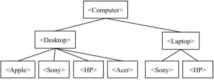
The following example explains the differences that arise with hierarchical class labels.Fig. 1shows a predefined hierarchy tree of product categories in an Internet store that sells computer-re-lated products. The class labels in lower levels represent more spe-cific concepts; therefore, they are more difficult to predict and the accuracy tends to be lower. The class labels in higher levels repre-sent more general concepts, so they are less specific but easier to predict. Hence, unlike the traditional DT classifiers, which only consider classification accuracy, our DT classifier must deal with the tradeoff between class specificity and classification accuracy. 0957-4174/$ - see front matterÓ2008 Elsevier Ltd. All rights reserved.

doi:10.1016/j.eswa.2008.05.044

*Corresponding author. Tel.: +886 3 4267266; fax: +886 3 4254604.

E-mail address:[email protected](Y.-L. Chen).

Contents lists available atScienceDirect

Expert Systems with Applications

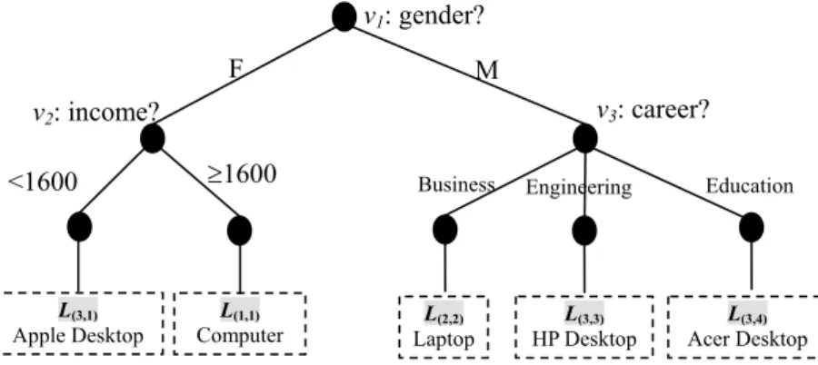
Suppose we want to build a decision classifier from data with class labels organized as shown inFig. 1. Assume thatFig. 2is a sample DT generated from the data. In the sample tree, half of nodev1’s data is labeledhApple Desktopiand the other halfhHP Laptopi, while half of node v2’s data is labeled hSony Laptopi and the other halfhHP Laptopi. Thus, the reasonable labels that we can assign to node v1 are hApple Desktopi, hHP Laptopi or

hComputeri; the first two have the highest class specificity and the last has the highest classification accuracy. It is useless to la-bel nodev1 ashDesktopi orhLaptopi, because these two are as accurate ashApple DesktopiandhHP Laptopibut are less specific. Similarly, the reasonable labels that we can assign to nodev2are

hSony Laptopi,hHP LaptopiorhLaptopi, because the first two have the highest class specificity and the last has the highest classifica-tion accuracy. Here, we do not labelv2ashComputeri, because it is dominated by labelhLaptopi.

The example above demonstrates several differences resulting from the use of hierarchical class labels. First, in selecting a split-ting attribute to grow the tree, we must consider not only accu-racy, but also class specificity. Second, in deciding when to stop growing a node and assign a label to the node, the distribution of data over the class hierarchical tree must be considered in or-der to determine a proper label. This paper proposes a novel classification algorithm to accommodate these differences by taking into account the distribution of class labels in the hierar-chical tree so that the precision and accuracy of a DT can be optimized.

The remainder of this paper is organized as follows: Section2

formalizes the problem, Section3 introduces the proposed algo-rithm, Section4presents the performance evaluation, and Section

5draws conclusions from the evaluation.

2. Problem definition

The following table, a training set of 16 hypothetical customers, is used throughout this paper to describe the problem, require-ments, and expected results. The goal is to build a DT from the data set. Let CHT denote the class hierarchical tree as shown inFig. 3. In

Table 1, each object of data will be associated with a specific con-cept label in CHT.

After applying the proposed algorithm to the input data of the training data set, we can construct a DT:T= (V,E), where Eis a set of branches andVis a set of nodes. Suppose the DT is like the one shown in Fig. 4. In the tree, each internal node corresponds to a decision on an attribute, and each branch corresponds to a pos-sible value of that attribute. The leaves are the final results of the

concept labels.

By using this tree, we can predict customers’ preferences. For example, if there is a female customer with an income of $1324, the tree indicates that she will be interested in anhApple Desktopi. The concept labelhApple Desktopiis at the most specific level of product categories. As a second example, consider a male customer who holds a post in Business. Tracing down the tree from the root, we reach a leaf with a more abstract product category,hLaptopi, so the DT shows that this customer will be interested in any kind of Laptop. The accuracy of the prediction in this case is still guaran-teed without losing too much precision. Finally, we can transform the DT into a set of ‘‘if-condition-then-label” rules by traversing each path of the tree from the root node to the leaf nodes, as shown inFig. 5.

Our goal is to construct a DT from the input data and a given class hierarchical tree CHT so that the two criteria, preciseness and accuracy, are maximized. Next, we formally define the problem.

Definition 1. Class hierarchical tree

The class hierarchical tree (CHT) is a tree whose root label covers all the concepts in the application domain. The concept of a parent label node will cover those of its child label nodes. For example,hLaptopiis a parent label node that covers the concepts of both of its child label nodes,hSony LaptopiandhHP Laptopi.

Let CHT ={L1,L2,. . .,Lh}, whereLidenotes theith concept level of CHT andhis the number of levels in CHT. Here,L1is the most abstract level, and L2,L3,. . .,Lh are the other levels, arranged in order of increasing specificity. We further defineLi= {L(i,j)|i= 1, ... ,h andj =1,. . .,mi}, whereL(i,j)means thejthconcept labelat leveli

Fig. 1.A hierarchy tree of product categories.

andmiis the number of concept labels at leveli. We let the number of all concept labels in CHT be denoted as |CHT|. We can then obtain the following information fromFig. 3.

|CHT| = 9

L1={L(1,1)} andm1= 1

L2={L(2,1),L(2,2)} andm2= 2

L3={L(3,1),L(3,2),L(3,3),L(3,4),L(3,5),L(3,6)} andm3= 6

During the DT construction process, the labels of the data in each node vb may have different distributions over the class hierarchical tree CHT. Based on how the labels of the data in node

vbare distributed over CHT, we can obtain a partial hierarchy tree of CHT to represent the label distribution of node vb, as shown below.

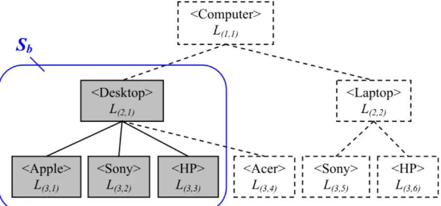
Definition 2. Partial hierarchical tree

LetSb #CHT be the smallest subtree in CHT that can cover the labels of all the data in node vb2DT. We call Sb the partial hierarchical tree of nodevb. More specifically, it can be represented asSb= {L(i,j)|i= 1, ... ,handj =1,. . .,mi}.

For example, if all the labels of the data invb2{hApple Desktopi,

hSony Desktopi, hHP Desktopi}, then we can obtain a partial hierarchical tree of nodevb,Sb# CHT, shown inFig. 6.

As another example, if all the labels of data in vc2{hApple

Desktopi,hSony Desktopi,hHP Laptopi}, then we will obtain another partial hierarchical tree of nodevc,Sc #CHT, shown inFig. 7.

We further defineH(Sb) as the number of levels inSb, and|Sb|as the number of all concept labels inSb.LetLbi denote the labels in

theith level inSb, andmbi denote the number of concept labels at

leveli inSb. By the example shown inFig. 7, we can obtain the following information aboutSc.

Sc={L(3,1),L(3,2),L(3,6),L(2,1),L(2,2),L(1,1)} |Sc| =6 H(Sc)=3 Lc 1¼ fL1;1gandmc1¼1 Lc 2¼ fL2;1;L2;2gandmc2¼2 Lc3 ¼ fLð3;1Þ;Lð3;2Þ;Lð3;6Þgandmc3¼3

LetDbe the training data set and |D| the number of records inD. We defineD(vb) as the data associated with nodevband |D(vb)| as the number of data records in nodevb. Furthermore, we let |D(b,i,j)| be the number of records in nodevbwhose labels are inL(i,j).

Suppose we use a DT to classify the data in the training data set. For each testing data entry, we traverse the DT to obtain an output category. If the actual class label of the testing data entry falls within the output category, then we know it is the correct product category for the testing data entry. We can use the percentage of correct predictions to measure the DTs accuracy. In addition, we can use the average level of all the predicted results in the CHT to measure the precision of the DT. Our goal is to construct a DT from the input data and a given class hierarchical tree CHT so that these two criteria, precision and accuracy, are maximized.

Fig. 3.A class hierarchical tree (CHT).

Table 1

Training set for 16 customers Customer ID Gender Customer’s career Customer’s income ($) Preferred product(class label)

1 F Business 1324 Apple desktop

2 F Business 1176 Apple desktop

3 F Engineering 1412 Apple desktop

4 F Engineering 1471 Apple desktop

5 F Education 1324 Apple desktop

6 F Education 1265 Apple desktop

7 F Engineering 1176 Apple desktop

8 F Education 1324 HP laptop

9 F Engineering 1912 Acer desktop

10 F Engineering 2059 Sony desktop

11 M Business 2353 Sony laptop

12 M Business 1412 Sony laptop

13 M Business 2206 HP laptop

14 M Business 1471 HP laptop

15 M Engineering 2206 HP desktop

16 M Education 1471 Acer desktop

Fig. 4.A DT built from the training data set inTable 1.

3. The HLC algorithm

The HLC (Hierarchical class Label Classifier) algorithm is de-signed to construct a DT from data with hierarchal class labels. It follows the standard framework of classical DT induction methods, such as ID3 (Quinlan, 1986) and C4.5 (Quinlan, 1993). The HLC pro-cess is:

1. HLC(Training Set D)

2. Initialize tree T and put all records of D in the root; 3. while (some leaf vb in T is a non-STOP node) 4. test if node vb can be stopped

5. if it can, mark vb as a STOP node, determine its concept label,

and exit

6. else for each attribute arofvb do

evaluate the appropriateness of splitting node vb with attributear

7. get the best split for it;

8. partition the node according to the best split; 9. endwhile;

10. returnT

The critical steps in the framework above, steps 4–5 and 6–7, deserve additional clarification. The former determines which nodes can stop growing and how to determine their concept labels,

while the latter determines the best attribute to use to split the current node into several child nodes. We will discuss steps 6–7 in Section3.1and steps 4–5 in Sections3.2 and 3.3.

Typically, for a non-STOP node, we have to select the most dis-criminatory attribute for splitting. In order to accomplish this, the information gain measure (entropy-based approach) is probably the most popular approach. Gain ratio (Agrawal, Ghosh, Imielinski, Iyer, & Swami, 1992; Agrawal, Imielinski, & Swami, 1993; Quinlan, 1986, 1993; Umano et al., 1994) and gini index (Mehta, Agrawal, & Rissanen, 1996; Shafer, Agrawal, & Mehta, 1996; Wang & Zaniolo, 2000) are two famous indices designed by this measure. By com-puting the indices, we can determine the appropriateness of an attribute, and the most appropriate attribute is chosen as the split-ting attribute for the current node.

Unfortunately, this approach could not be used in our problem, because it cannot handle hierarchical class labels while construct-ing a DT. Since the proposed algorithm is designed to construct a DT with hierarchical class labels, we have to consider the distribu-tion of the labels of the data over the class hierarchical tree while developing the DT. Therefore, the proposed measure should be capable of dealing with hierarchical class labels.

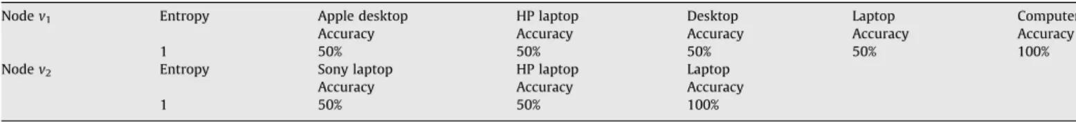
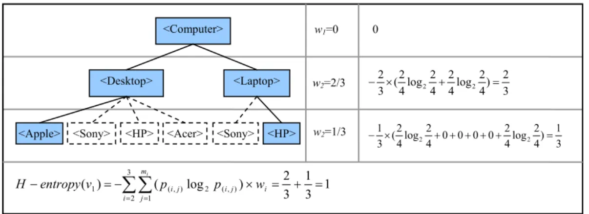
For example, suppose the data in nodesv1andv2is shown in

Tables 2 and 3, respectively. Traditionally, the entropy value, a well-known measure, would be used to determine the appropri-ateness of a current node in constructing a DT. If we use an entro-py-based approach to measure the appropriateness of nodesv1and

v2, we find that both nodes are equally appropriate, because their entropy values are the same. Moreover, no matter which label is

Fig. 6.A partial hierarchical treeSbof nodevb.

assigned to the current node, its accuracy is at most 50%.Table 4

shows the results.

Assume that the class labels can be organized in a class hierar-chical tree, as shown in Fig. 3. The partial hierarchical tress of nodesv1andv2,S1andS2, are shown inFigs. 8-1 and 8-2, respec-tively. There are five possible class labels that can be assigned to

node v1, and three to nodev2.Table 5shows which labels can be assigned to which nodes and the accuracy of these assignments. Note that the label distribution in nodev2is better than inv1. This is due to the fact that when the attached labels of both nodes have the same accuracy, the concept label attached to nodev2would be more specific than that attached tov1. For example, if we attach la-belshComputeritov1 andhLaptopitov2, nodev2’s label would then be more specific than that ofv1, even though they have the same accuracy.

The example above indicates that the traditional entropy mea-sure is unable to meamea-sure the appropriateness of nodes when the class labels are hierarchical. To overcome this weakness, this paper proposes not only a new entropy measure suitable for measuring the appropriateness of a node with hierarchical class labels, but also a new strategy to determine the most suitable concept label in the hierarchy for a leaf node.

3.1. Attribute selection measure

An attribute selection measure is a heuristic to measure which attribute is the most discriminatory to split a current node. Many algorithms for DT induction, such as ID3 (Quinlan, 1986) and C4.5 (Quinlan, 1993), are suitable for problems with flat nominal classes, and the entropy-based approach is probably the most pop-ular approach to selecting the most discriminatory attribute for splitting.

In view of the weakness of the traditional entropy-based meth-od discussed above, we propose a new measure, called hierarchical-entropy value, by modifying the traditional entropy measure. It can help measure the appropriateness of a node with respect to the gi-ven class hierarchical tree.

3.1.1. Hierarchical-entropy value

The hierarchical-entropy value of a nodevbcan be denoted as

Hentropy(vb), and can be computed with the following equation:

HentropyðvbÞ ¼ Xh i¼k Xmi j¼1 ðpði;jÞlog2pði;jÞÞ wi; wherek¼hHðSbÞ þ2

Note thatp(i,j)is the probability that an arbitrary tuple inD(vb) be-longs to concept labelL(i,j), andp(i,j)can be estimated bypði;jÞ¼

jDðb;i;jÞj

jDðvbÞj.

Letwibe the weight of levelLiin tree CHT. SinceL1is the root label of CHT, the weight ofL1 is set to w1= 0. Assumew1,w2,

w3,. . .,whis an arithmetic sequence andPhi¼1wi¼1. The following relation can then be used to computewi.Table 6shows the value of

wiwhenhis varied from 3 to 5. Table 4

The information ofv1andv2

Nodev1 Entropy Apple desktop HP laptop

1 Accuracy Accuracy

50% 50%

Nodev2 Entropy Sony laptop HP laptop

1 Accuracy Accuracy

50% 50%

Table 5

The information ofv1andv2with hierarchical class labels

Nodev1 Entropy Apple desktop HP laptop Desktop Laptop Computer

Accuracy Accuracy Accuracy Accuracy Accuracy

1 50% 50% 50% 50% 100%

Nodev2 Entropy Sony laptop HP laptop Laptop

Accuracy Accuracy Accuracy

1 50% 50% 100%

Table 3

The tuples of customers’ preferences within nodev2

ID Customer’s career Customer’s education Preference(class label)

11 Education Mid Sony laptop

12 Official Mid Sony laptop

13 Education High HP laptop

14 Business High HP laptop

Fig. 8-1.Partial hierarchical class label of nodev1.

Fig. 8-2.Partial hierarchical class label of nodev2.

Table 6

The weight setting forwiby varyinghfrom 3 to 5

h= 3 h= 4 h= 5 w1 0 w1 0 w1 0 w2 2/3 w2 3/6 w2 4/10 w3 1/3 w3 2/6 w3 3/10 w4 1/6 w4 2/10 w5 1/10 Table 2

The tuples of customers’ preferences within a nodev1

ID Customer’s career Customer’s education Preference(class label)

1 Official Mid Apple desktop

2 Business Low Apple desktop

3 Business Low HP laptop

wi¼ ðhiþ1Þ

2

hðh1Þ; wherei>1

We use the data inTables2 and 3 to illustrate the concept of hier-archical-entropy value and howHentropy(v1) and Hentropy(v2) are

calculated.FromTable 2, we have |D(v1)| = 4, |D(1,3,1)| = 2, |D(1,3,6)| =

2, |D(1,2,1)| = 2 and |D(1,2,2)| = 2. By using the structure inFig. 8-1,

we can then obtain H(S1) = 3,k= 33 + 2 = 2,m1= 1,m2= 2 and

m3= 6. Based on this information, we can compute the hierarchi-cal-entropy value ofv1as shown inFig. 9-1.

Likewise, from Table 3, we have |D(v2)| = 4, |D(1,3,5)| = 2,

|D(1,3,6)| = 2 and |D(1,2,2)| = 4. By using the structure inFig. 8-2, we

obtain H(S2) = 2, k= 32 + 2 = 3, m1= 1, m2= 2 and m3= 6. We can then compute the hierarchical-entropy value ofv2as shown inFig. 9-2.

As shown in Fig. 9, we have Hentropy(v1) = 1 and

Hentro-py(v2) = 1/3. Since a lower entropy value implies less chaos, the appropriateness of nodev2is better than that of nodev1.This result

indicates that by using the new hierarchical-entropy measure, the appropriateness of a node in a CHT can be properly measured.

3.1.2. Hierarchical information gain

Next, we decide whether an attribute is a good splitting attri-bute according to how much hierarchical information is gained by splitting the node through the attribute. We first define what the hierarchical information gain is, and we then use it to develop a method for choosing the best splitting attribute.

The hierarchical information gain is used to select a test attri-butearto split the current nodevb, and can be denoted as

H-info-Gain(ar,vb). Let vx denote a child node obtained by splitting vb through test attribute ar. The hierarchical information gain can then be computed as follows:

HinfoGainðar;

m

m

for allx jDð

m

jDðvbÞjHentropyð

m

Fig. 9-1.The appropriateness of nodev1.

Fig. 9-2.The appropriateness of node v2.

Our goal is to select the attribute with the highestH-infoGainvalue, which is chosen as the next test attribute for the current node. As shown inFig. 10, theChooseAttributefunction finds the most appro-priate attribute to split.

3.2. Stop criteria

For the labels at the bottom level, letmajoritybe the label with the most data invb, and letpercent(vb,majority) be the percentage of data invbwhose labels aremajority. If the following conditions are met, we stop growing nodevb; otherwise, the node must be ex-panded further.

1. If the entire set of attributes has been used in the path from root down tovb, thenvbis a stop node.

2. Ifpercent(vb,majority) >fM, thenvbis a stop node, wherefMis a given threshold.

3. If |D(vb)|/|D|hfD, a given threshold, thenvbis a stop node. 4. If theH-infoGainof all unused attributes is no more than 0, then

we also treatvbas a stop node.

Once stopped, we will assign a concept label to a stop nodevbto cover most of the data without losing too much precision. We accomplish this by using the functiongetLabel, detailed in the next section.

3.3. Label assignment

In this section, we introduce a heuristic for assigning a class la-bel when a node matches the stop criteria. The goal is to use the concept label in the class hierarchical tree with the highest accu-racy and precision to label the node.

As discussed above, the higher the predicted class label in the class hierarchical tree, the lower the classification error.

Unfortu-nately, such classification becomes less specific and, as a conse-quence, less useful. Therefore, we must deal with the tradeoff between class specificity and classification accuracy.

The functiongetLabel, shown inFig. 11, provides an automatic way to extract a proper concept label from the hierarchical tree to label a leaf node. Each concept label of a leaf nodevbhas three vital indices:

(1) Accuracy: letacc(L(i,j)) be the prediction accuracy of a leaf node with labelL(i,j), which can be computed as follows: accðLði;jÞÞ ¼

jDðb;i;jÞj jDð

m

(2) Precision: the degree of precision of a leaf node with label

L(i,j), which can be computed as follows: preðLði;jÞÞ ¼loghðiþ1Þ:

(3) Score: theScore(L(i,j)) is used to indicate how well a concept label will be able to label a leaf node. From the partial hier-archical tree of a node, any concept label in the correspond-ing partial hierarchy can have a Scorevalue. The concept label with the highestScorewill be used to label a leaf node. TheScoreof each concept label in nodevbcan be computed as follows:

ScoreðLði;jÞÞ ¼accðLði;jÞÞ preðLði;jÞÞ

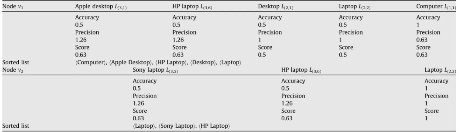
Applying the function getLabel to the information shown in

Table 5, we can obtain the accuracy, precision, and score values for each concept label of nodesv1and v2. The results are listed in Table 7. In node v2, after sorting the concept labels first by their score value and then by their accuracy value, the label

hLaptopihas the largest score value and should be assigned to nodev2. Similarly, in nodev1, the most appropriate concept label ishComputeri.

Table 7

The detail information of each concept label withinv1andv2

Nodev1 Apple desktopL(3,1) HP laptopL(3,6) DesktopL(2,1) LaptopL(2,2) ComputerL(1,1)

Accuracy Accuracy Accuracy Accuracy Accuracy

0.5 0.5 0.5 0.5 1

Precision Precision Precision Precision Precision

1.26 1.26 1 1 0.63

Score Score Score Score Score

0.63 0.63 0.5 0.5 0.63

Sorted list hComputeri,hApple Desktopi,hHP Laptopi,hDesktopi,hLaptopi

Nodev2 Sony laptopL(3,5) HP laptopL(3,6) LaptopL(2,2)

Accuracy Accuracy Accuracy

0.5 0.5 1

Precision Precision Precision

1.26 1.26 1

Score Score Score

0.63 0.63 1

Sorted list hLaptopi,hSony Laptopi,hHP Laptopi

4. Performance evaluation

To evaluate the performance, the algorithm was implemented in JAVA language and tested on a Pentium 4–2 GHz Microsoft Win-dows XP system with 1024 MB of RAM.

We conducted an empirical study to demonstrate that the pro-posed method can achieve a good result in both predictive accu-racy and predictive precision. Two real-world data sets were used in the experiments and are listed inTable 8. The data sets can be downloaded freely from a popular web site of U.C. Irvine databases (Murphy & Aha, 1994). We chose these two data sets from the U.C. Irvine repository because their concept labels could be naturally organized into a tree structure.

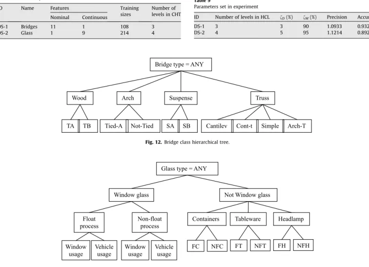
In the Bridges data set, the learning task is to predict the type of bridge. Among these 108 instances, the Bridges dataset has ten concept labels and can be grouped into a three-level class hierar-chical tree as shown inFig. 12.

In the Glass data set, there are 214 instances, and the learning task is to predict the type of glass. The set of 10 concept labels have been grouped into a four-level class hierarchical tree as shown in

Fig. 13.

In this experiment, we used two criteria to compare the perfor-mances of different algorithms: (1) accuracy, which is the percent-age of future data that can be correctly classified into the right concept label, and (2) precision, which is a measure of specificity of the label data can be assigned to. We express precision as the averagePrecisionvalue of all test data. As defined in Section3.3,

the larger the precision value, the more specific the label. As a re-sult, a larger precision value implies a more specific and precise result.

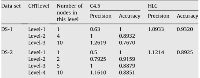
As stated in Section3.2, two thresholds,fMandfD, are used in the HLC algorithm to control a node’s growth. In the algorithm, one stop condition is if the amount of data in the node is small en-ough (controlled byfD), and the other stop condition is if the per-centage of data with majority label in a current node is large enough (controlled byfM). In our pretest experiment, we observed the results of the HLC algorithm by varying the values of these two parameters. After the pretest, we then selected the optimal combi-nation of parameters for each data set and let them be the specified thresholds in constructing the DT, as shown inTable 9. The last two columns show the precision and accuracy results for each data set by setting these specific thresholds.

To highlight the tradeoffs between predictive accuracy and pre-dictive precision of the resulting hierarchical concept labels, and to explore the performance of our proposed method, we chose a well-known decision tree system, C4.5, to compare with our method, HLC. Since C4.5 cannot handle hierarchical class labels, we com-puted the accuracy for every level of the CHT of each data set. Since the concept tree in DS-1 has three-levels and that in DS-2 has four-levels, there are seven total accuracy values for C4.5. The results of this comparison are shown inFig. 14.

InFig. 14, the HLCs performance data falls into the upper right-hand part of the graph. This means that the HLC algorithm can achieve higher accuracy and better precision simultaneously. By

Fig. 12.Bridge class hierarchical tree.

Fig. 13.Glass class hierarchical tree.

Table 9

Parameters set in experiment

ID Number of levels in HCL fD(%) fM(%) Precision Accuracy

DS-1 3 3 90 1.0933 0.9320

DS-2 4 5 95 1.1214 0.8925

Table 8

Summarized descriptions of data sets

ID Name Features Training

sizes Number of levels in CHT Nominal Continuous DS-1 Bridges 11 1 108 3 DS-2 Glass 1 9 214 4

carefully examining the C4.5 performance data level-by-level, we find that when accuracy is high, precision becomes low, and vice-versa. This is because the traditional decision tree classifier does not consider data with hierarchical class labels, and thus it cannot handle the tradeoffs between accuracy and precision. On the other hand, since our aim is to construct a DT from data with a class hierarchical tree, the ability to optimize the tradeoff be-tween these two criteria is deeply embedded into the design of our algorithm. The results in Fig. 14 indicate that our design achieved this goal.

We now compare the detailed precision and accuracy results of HLC and C4.5, shown inTable 10. HLC retains the same precision and accuracy for each data set at different levels of CHT because HLC has already considered the distribution of the concept labels over the CHT while developing the decision tree, rather than exam-ining the performance data level-by-level.

For classification accuracy, the C4.5 algorithm is slightly better than HCL in dataset DS-1 only when the level of CHT is 1, which means that all the labels are generalized into a single label. Simi-larly, the accuracy of C4.5 can be better than HCL in dataset DS-2 if the level of CHT is below 2, which means that all the labels are generalized into no more than two labels. These results indicate that the accuracy of C4.5 is very unlikely to be better than HCL without sacrificing precision.

For classification precision, the C4.5 algorithm can be slightly better than HCL in dataset DS-1 only when the level of CHT is at level 3, which is the bottom level of the concept tree. Similarly, the accuracy of C4.5 can be better than HCL in dataset DS-2 if the level of CHT is at level 4, which means all the labels are kept in the most primitive form. These results indicate that the preci-sion of C4.5 is very unlikely to be better than HCL without sacrific-ing accuracy.

5. Conclusions and future work

Most decision tree classifiers are designed to classify the data whose class labels are categorical or Boolean. To the best of our knowledge, no previous research has considered the induction of a decision tree from data with hierarchical class labels. This paper proposed a novel classification algorithm for learning decision tree classifiers from data with hierarchical class labels.

To evaluate the performance of the proposed method, HLC, experiments were performed using two real-world datasets from the U.C. Irvine repository. According to the experimental results, HCL is superior to the traditional decision tree classifier, C4.5, be-cause it is efficient and effective in both prediction accuracy and prediction specificity.

This work can be extended in several ways. First, if there exists distances between concept labels in the hierarchical tree, further work should be undertaken to design a decision tree that not only maximizes the accuracy and precision, but also minimizes the dis-tance between the real label and predicted label. Second, if the data with hierarchical labels could be extended as a directed acyclic graph (DAG), we could explore building decision trees that classify data with more complex analyses. In DAG structures, a child node may have more than one parent; hence, the class labels in deeper levels may be induced from more instances than their ancestors. In all the above extensions, as in this paper, the goal is to find the best tradeoff between precision and accuracy.

References

Adomavicius, G., & Tuzhilin, A. (2001). Using data mining methods to build customer profiles.IEEE Computer(February), 74–82.

Agrawal, R., Ghosh, S., Imielinski, T., Iyer, B., & Swami, A. (1992). An interval classifier for database mining applications. In Proceedings of the 18th international conference on very large databases(pp. 560– 573). Vancouver, BC. Agrawal, R., Imielinski, T., & Swami, A. (1993). Database mining: A performance

perspective. IEEE Transactions on Knowledge and Data Engineering, 5(6), 914–925.

Berry, Michael J. A., & Linoff, Gordon S. (2000).Mastering data mining: The art & science of customer relationship management. New York: Wiley.

Bonchi, F., Giannotti, F., Mainetto, G., & Pedresch, D. (1999). A classification-based methodology for planning audit strategies in fraud detection. In:Proceedings of the fifth ACM SIGKDD international conference on knowledge discovery and data mining(pp. 175–184).

Breiman, L., Friedman, J., Olshen, R., & Stone, C. (1993).Classification and regression trees. New York: Chapman & Hall.

Brodley, C. E., & Utgoff, P. E. (1995). Multivariate decision trees.Machine Learning, 19, 45–77.

Chen, Y. L., Hsu, C. L., & Chou, S. C. (2003). Constructing a valued and multi-labeled decision tree.Expert Systems with Applications, 25, 199–209.

Cho, Y. H., Kim, J. K., & Kim, S. H. (2002). A personalized recommender system based on web usage mining and decision tree induction. Expert Systems with Applications, 23, 329–342.

Duda, R., Hart, P., & Stork, D. (2001).Pattern classification(2nd ed.). New York: Wiley.

Durkin, J. (1992). Induction via ID3.AI Expert, 7, 48–53.

Fayyad, U. M., & Irani, K. B. (1992). On the handling of continuous-values attributes in decision tree generation.Machine Learning, 8, 87–102.

Kushmerick, N. (1999). Learning to remove Internet advertisements. In:Third international conference on autonomous agents.

Li, X. B., Sweigart, J., Teng, J., Donohue, J., & Thombs, L. (2001). A dynamic programming based pruning method for decision trees.INFORMS Journal on Computing, 13, 332–344.

Mehta, M., Agrawal, R., & Rissanen, J. (1996). SLIQ: A fast scalable classifier for data mining. InProceedings of the fifth international conference on extending database technology(pp. 18–32).

Murphy, P. M., Aha, D. W. (1994). UCI repository of machine learning database, for information contact [email protected].

Piramuthu, S. (1999). Feature selection for financial credit-risk evaluation decisions.

INFORMS Journal on Computing, 11, 258–266.

Quinlan, J. R. (1986). Induction on decision trees.Machine Learning, 1, 81–106. Quinlan, J. R. (1993). C4.5: Programs for machine learning. Kluwer Academic

Publishers.

Quinlan, J. R. (1996). Improved use of continuous attributes in C45.Artificial Intelligence, 4, 77–90.

Shafer, J. C., Agrawal, R., & Mehta, M., (1996). SPRINT: A scalable parallel classifier for data mining. InProceedings of the 22nd international conference on very large databases(pp. 544–555).

Table 10

The precision and accuracy in C4.5 and HLC Data set CHTlevel Number of

nodes in this level

C4.5 HLC

Precision Accuracy Precision Accuracy

DS-1 Level-1 1 0.63 1 1.0933 0.9320 Level-2 4 1 0.8932 Level-3 10 1.2619 0.7670 DS-2 Level-1 1 0.5 1 1.1214 0.8925 Level-2 2 0.7925 0.9159 Level-3 5 1 0.8879 Level-4 10 1.1610 0.8851 0.4 0.5 0.6 0.7 0.8 0.9 1 1.1 1.2 1.3 1.4 0.75 0.8 0.85 0.9 0.95 1 1.05 Accuracy Pricision C4.5-DS-1 C4.5-DS-2 HLC-DS-1 HLC-DS-2

Shaw, M., Subramaniam, C., Tan, G. W., & Welge, M. E. (2001). Knowledge management and data mining for marketing.Decision Support Systems, 31, 127–137.

Thearling, K. (1999). Data mining and CRM: Zeroing in on your best customers.

dmDitrect(December), 20.

Umano, M., Okamoto, H., Hatono, I., Tamura, H., Kawachi, F., Umedzu, S., & Kinoshita, J., (1994). Fuzzy decision trees by fuzzy ID3 algorithm and its application to diagnosis systems. InProceedings of the third IEEE international conference on fuzzy systems(Vol. 3, pp. 2113–2118), Orlando, FL.

van der Putten, P. (1999). Data mining in direct marketing databases. In W. Baets (Ed.),Complexity and management: A collection of essays. Singapore: World Scientific Publishers.

Wang, H., & Zaniolo, C (2000). CMP: A fast decision tree classifier using multivariate predictions. In Proceedings of the 16th international conference on data engineering(pp. 449–460), Bombay, India.

Wu, F., Zhang, J., & Honavar, V. (2005). Learning classifiers using hierarchically structured class taxonomies. In Proceedings of symposium on abstraction reformulation, and approximation(pp. 313–320).

Yang, Y., & Pedersen, J. O. (1997). A comparative study on feature selection in text categorization. InProceedings of the 14th international conference on machine learning.

Zamir, O., & Etzioni, O. (1998). Web document clustering: A feasibility demonstration. Research and Development in Information Retrieval, 46–54.