Kernel-based adaptive estimation: multidimensional and state-space approaches

(1)

M

ULTIDIMENSIONAL AND

S

TATE-S

PACE

A

PPROACHES

by

FELIPE

A. TOBAR

A Thesis submitted in fulfilment of requirements for the degree of Doctor of Philosophy of Imperial College London

Communication and Signal Processing Group Department of Electrical and Electronic Engineering

Imperial College London 2014

(2)

(3)

Abstract

Several disciplines, from engineering to social sciences, critically depend on adaptive signal estimation to either remove observation noise (filtering), or to approximate quan-tities before they become available (prediction). When an optimal estimator cannot be expressed in closed form, e.g. due to model uncertainty or complexity, machine learn-ing algorithms have proven to successfullylearn a model which captures rich relation-ships from large datasets. This thesis proposes two novel approaches to signal estimation based on support vector regression (SVR): high-dimensional kernel learning (HDKL) and kernel-based state-spaces modelling (KSSM).

In real-world applications, signal dynamics usually depend on both time and the value of the signal itself. The HDKL concept extends the standard, single-kernel, SVR estimation approach by considering a feature space constructed as an ensemble of real-valued feature spaces; the resulting feature space provides highly-localised estimation by averaging the subkernels estimates and is well-suited for multichannel signals, as it captures interchannel data-dependency. This thesis then provides a rigorous account for the existence of such higher-dimensional RKHS and their corresponding kernels by considering the complex-, quaternion- and vector-valued cases.

Current kernel adaptive filters employ nonlinear autoregressive models and ex-press the current value of the signal as a function of past values with added noise. The motivation for the second main contribution of this thesis is to depart from this class of models and propose a state-space model designed using kernels (KSSM), whereby the signal of interest is a latent state and the observations are noisy measurements of the hidden process. This formulation allows for jointly estimating the signal (state) and the parameters, and is robust to observation noise. The posterior density of the kernel mixing parameters is then found in an unsupervised fashion using Markov chain Monte Carlo and particle filters, and both the offline and online cases are addressed.

The capabilities of the proposed algorithms are initially illustrated by simulation examples using synthetic data in a controlled environment. Finally, both the HDKL and the KSSM approaches are validated in the estimation of real-world signals includ-ing body-motion trajectories, bivariate wind speed, point-of-gaze location, and national grid frequency.

(4)

Acknowledgments

I have been very fortunate to be part of the Signal Processing and Communications Group (CSP) at Imperial College London for almost four years. I am deeply grateful to my super-visor, Prof. Danilo P. Mandic, for encouraging rigour in both content and presentation of my work, for always taking the time to discuss research ideas and read my manuscripts, and for the financial support he provided. Danilo has not only been my mentor in the fascinating field of Adaptive Signal Processing, he has also shared his expertise with me on more worldly arts such as bicycle and motorcycle riding, and life in London.

I am indebted to Prof. Sun-Yuan Kung, Princeton University, for his advice on multikernel learning, and to Prof. Petar M. Djuri´c, Stony Brook University, for guidance on sequential Monte Carlo methods; the collaborations with Profs Kung and Djuri´c have greatly benefitted this thesis and its related publications. I am also thankful to my exam-iners, Prof. Jose C. Principe, University of Florida, and Prof. Anthony G. Constantinides, Imperial College London, for enlightening comments and encouraging feedback.

From Imperial, I would also like to thank to my fellow lab mates in CSP, David Looney and Jon O ñativia, for their friendship and company in academic matters, such as the quest for elegance when producing research material and the infinite proofread-ing, as well as in not-so-academic ones, such as the sobre mesa coffees and some other types of beverages around South Kensington. Special thanks to my Chilean friends: Luis Pizarro, Javier Correa and Diego Oyarz ún (at Imperial), and Diego Mu ñoz-Carpintero (at Oxford); they have made the stay away from home much easier.

From Universidad de Chile, I want to express my sincere gratitude to Dr. Marcos E. Orchard for his guidance prior to my PhD studies and Prof. Manuel A. Duarte be-fore that, they encouraged my initiation into research and remain a source of guidance on academic life. I am also grateful to Chile’s National Commission for Scientific and Technological Research (CONICYT) for funding my PhD studies.

Finally, I want to thank my parents, for their infinite love and support in every possible manner; my sister, for providing wise pieces of advice on life matters; and P´ıa, for always being by my side.

Felipe A. Tobar. London, August 2014.

(5)

List of Figures

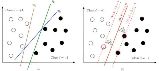
2.1 Classification of linearly separable data. The left plot shows how an infi-nite number of planes classify the data samples, while the right plot shows the (unique) maximum margin separating plane and the support vectors (with red shadows). . . 28 2.2 Classification of non-linearly-separable data. The left plot shows the

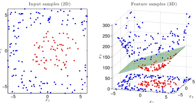
orig-inal samples in R2 corresponding to classes red and blue, while the right

plot shows both original and feature samples inR3with the corresponding

separating plane. . . 29 2.3 RBF kernels defined onR2. The triangular and Epanechnikov kernels are

rotation invariant and have finite support, the Gaussian kernel is invariant and has infinite support, and the Mahalanobis kernel is rotation-sensitive and has infinite support. . . 34 3.1 Estimation of the processdtas a projection onto the space of linear

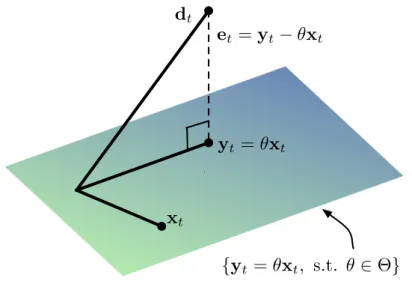
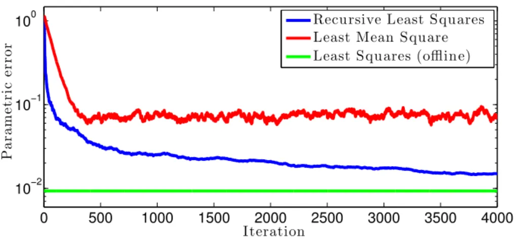
estima-torsyt=θxt, θ∈Θ. . . 39 3.2 Performance of adaptive filters for system identification: Norm of the

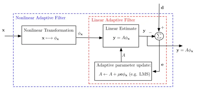
mis-alignment (parametric error) as a function of iteration number. . . 46 3.3 Diagram of an adaptive filter that is nonlinear in the input (x) and linear

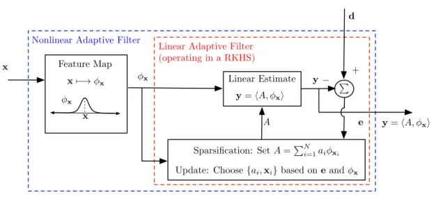
in the parameters (A). This filter is constructed by applying a nonlinear transformation on the input and then performing adaptive filtering using the transformed sample. . . 47 3.4 Kernel adaptive filter. The input is mapped to an infinite-dimensional

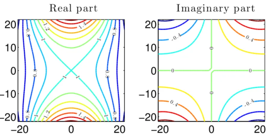
fea-ture space, and then linear adaptive filtering is performed on the feafea-tures. This requires the update of both mixing parameters and support vectors. . 48 4.1 Contour plot of real and imaginary parts of the complex Gaussian kernel

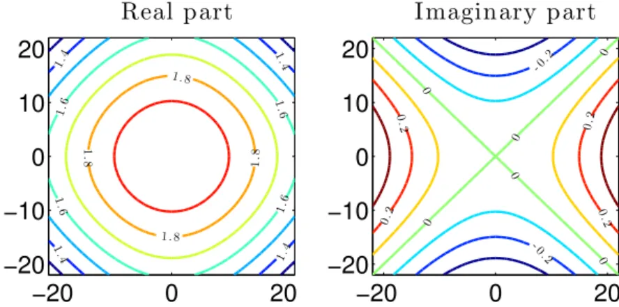
KCGin eq. (4.1) andσ2 = 103. . . 58 4.2 Independent complex kernel in eq. (4.1) generated from a real-valued

(10)

4.3 Real (left) and i-imaginary (right) parts of KQP. The colourmap is dark blue for−13·103_{, white for the interval}_[₋₁₀_,_{10], and red for}₁₃_·₁₀3_with

a logarithmic RGB interpolation. . . 70 4.4 Real (left) and i-imaginary (right) parts of KQG. The colourmap is dark

blue for−7·10−4_{, white for 0, and red for}₇_·₁₀4_{, with a logarithmic RGB}

interpolation. . . 72 4.5 MSE ±0.5 standard deviations for kernel algorithms as a function of the

number of support vectors in the estimation of both uncorrelated (top,

A = 0.6808, B= 0.1157) and correlated (bottom,A= 0.6808 +i0.07321 +

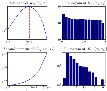
j0.6222−k0.2157, B= 0.1157 +i0.1208 +j0.8425−k0.5121) AR(1) processes. 73 4.6 Choice of kernel parameters (red)ARandAQbased on the second moment

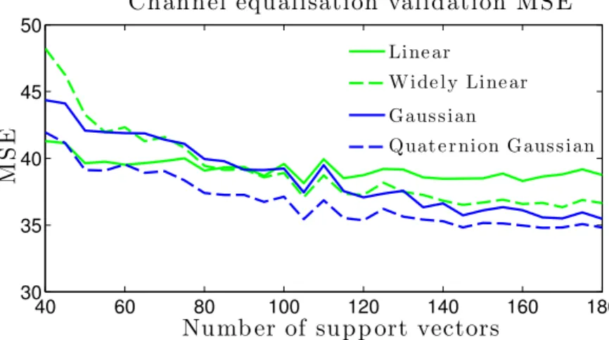
of the kernel evaluations and histograms corresponding to the chosen pa-rameters. . . 75 4.7 Training MSE of ridge regression algorithms for channel equalisation. . . 76 4.8 Validation MSE of ridge regression algorithms for channel equalisation. . 76 5.2 Training error norm for different values of the kernel width. The global

minimum has the value of3.11and is reached forσ = 1.48. . . 88 5.1 A nonlinear function and support vectors. . . 88 5.3 Nonlinear function estimation using mono- and multi-kernel ridge

regres-sion algorithms. . . 89 5.4 Trivariate original signal and KLMS estimates. . . 90 5.5 Time varying magnitude of the weight matrix for all the three

imple-mented kernel algorithms. . . 91 5.6 Averaged MSE and dictionary size (in number of samples) over 30 trials

for the kernel algorithms. . . 92 7.1 Observed process for the system in eq. (7.24). . . 114 7.2 Original state-transition function, state samples and kernel-based

approx-imation. . . 115 7.3 Value of the posterior p(a_|y1:40) for the supervised solution and the

sam-ples generated by the proposed method. . . 116 7.4 Prediction using the proposed KSSM. . . 116 7.5 The state-transition function of the system in (7.26) is time-varying

be-tween t = 30 andt = 60, and constant for t < 30 (system stable) and fort >60(system unstable). . . 118 7.6 KSSM estimate (mean and standard deviation) of the time-varying

state-transition function in (7.26) fort = 30andt = 90. The true state samples are plotted with red borders for the regions[1,30](green fill) and[61,90] (blue fill). . . 119

(11)

7.7 Filtered state signal using the KSSM and SIR particle filter. The original state is shown in blue and the posterior mean in red, with a one-standard-deviation confidence interval in light red. . . 120 8.1 Original north-south wind speed component and KLMS estimates. . . 124 8.2 Input sample deviation for the low, medium, and high dynamics wind

regime. . . 125 8.3 Original bivariate wind signal and its KLMS estimates for the low

dynam-ics region. . . 126 8.4 Weight magnitudes for the kernels within the MKLMS algorithm,

evalu-ated for mixed regime wind, using the proposed adaptive sparsification criteria. . . 126 8.5 Dictionary size for all kernel algorithms for the prediction of mixed-regime

wind using the proposed adaptive sparsification criteria. . . 127 8.6 Averaged MSE and dictionary size over 30 trials of combined low, medium

and high dynamics regions. . . 128 8.7 Inertial body sensor setting. [Left]Fixed coordinate system (red), sensor

coordinate system (blue) and Euler angles (green). [Right]A 3D inertial body sensor at the right wrist. . . 129 8.8 Raw angle measurements and considered features. [Top]Original

discon-tinuous angle recording and [Bottom]the corresponding continuous sine and cosine mapping. Observe that in the right (left) circle only cosine (sine) preserves the dynamics of the angle signal accurately. . . 130 8.9 Body sensor signal tracking: Angle features(sinθ,cosθ)and KRR estimates. 131 8.10 Performance of KRR algorithms for body sensor signal tracking as a

func-tion of the number of support vectors. . . 132 8.11 Computation time of KRR algorithms for body sensor signal tracking. . . 132 8.12 Average running time and standard deviation for kernel algorithms as a

function of the number of support vectors. . . 133 8.13 MSE and standard deviation for kernel algorithms as a function of number

of support vectors. . . 134 8.14 Performances of kernel algorithms for gaze prediction. . . 135 8.15 Kernel algorithms prediction and original gaze signal for KNLMS, KRLS

and KSSM. . . 135 8.16 Original signal and kernel SSM densities for the prediction of gaze signals. 136 8.17 Online estimation of the state-transition function fort_∈[2,7]. The hidden

state samples are shown in red. . . 137 8.18 Kernel predictions of the UK National Grid frequency. The original signal

is shown in red, the KLMS prediction in red, the KSSM prediction in blue, and the one-standard-deviation confidence interval in light blue. . . 138

(12)

(13)

List of Tables

5.1 Computational complexity of weight computation for KRR algorithms . . 87 5.2 Estimation error for mono- and multi-kernel ridge regression algorithms. 89 5.3 Averaged prediction gains and running times for the Gaussian KLMS,

tri-angular KLMS and MKLMS. . . 91 7.1 Prediction performance of kernel algorithms . . . 117 8.1 10 log₁₀(MSE) for wind prediction (last 500 samples). . . 124 8.2 Averaged prediction gains for the low-fitted KLMS (LF), medium-fitted

KLMS (MF), high-fitted KLMS (HF), and MKLMS for all three dynamic regions . . . 127 8.3 Averaged running time (in seconds) for the low-fitted KLMS (LF),

medium-fitted KLMS (MF), high-fitted KLMS (HF), and MKLMS for all three dynamic regions . . . 128

(14)

Statement of Originality

I declare that this is an original thesis and it is entirely based on my own work. I ac-knowledge the sources in every instance where I used the ideas of other writers. This thesis was not and will not be submitted to any other university or institution for fulfill-ing the requirements of a degree.

(15)

Copyright Declaration

The copyright of this thesis rests with the author and is made available under a Creative Commons Attribution Non-Commercial No Derivatives licence. Researchers are free to copy, distribute or transmit the thesis on the condition that they attribute it, that they do not use it for commercial purposes and that they do not alter, transform or build upon it. For any reuse or redistribution, researchers must make clear to others the licence terms of this work

(16)

Publications

The following publications support the material given in this thesis.

Submitted

• F. Tobar and D. Mandic, “High-Dimensional Kernel Regression: A Guide for Prac-titioners,” Book chapter, Festschrift.

• F. Tobar, P. Djuri´c and D. Mandic, “Unsupervised state-space modelling using re-producing kernels,”IEEE Transactions on Signal Processing, 2014.

Peer-reviewed journals

• F. Tobar, S.-Y. Kung, and D. Mandic, “Multikernel least mean square algorithm,” IEEE Transactions on Neural Networks and Learning Systems, vol. 25, no. 2, pp. 265-277, 2014.

• F. Tobar and D. Mandic, “Quaternion reproducing kernel Hilbert spaces: Existence and uniqueness conditions,”IEEE Transactions on Information Theory, vol. 60, no. 9, pp. 5736-5749, 2014.

Peer-reviewed conferences

• F. Tobar, A. Kuh, and D. Mandic, “A novel augmented complex valued kernel LMS,” inProc. of the 7th IEEE Sensor Array and Multichannel Signal Processing Work-shop, 2012, pp. 473-476.

• F. Tobar and D. Mandic, “Multikernel least squares estimation,” in Proc. of the Sensor Signal Processing for Defence Conference, 2012, pp. 1-5.

• F. Tobar and D. Mandic, “The quaternion kernel least squares,” in Proc. of IEEE International Conference on Acoustics, Speech and Signal Processing, 2013, pp. 6128-6132.

• F. Tobar and D. Mandic, “A particle filtering based kernel HMM predictor,” inProc. of IEEE International Conference on Acoustics, Speech and Signal Processing, 2014, pp. 8019-8023.

(17)

Abbreviations and Symbols

RKHS Reproducing kernel Hilbert Space

KLMS Kernel least mean square

KRLS Kernel recursive least squares

KRR Kernel ridge regression

KSSM Kernel state space model

MSE Mean square error

MMSE Minimum mean square estimate

QRKHS Quaternion Reproducing kernel Hilbert Space

RBF Radial basis function

SSM State space model

SVM Support vector machine

SVR Support vector regression

{A_}i ithentry of vectorA

A1:t={A1, . . . ,At} Collection of samplesA1, . . . ,At

D=_{s1_{, . . . ,}_sN_} _{Dictionary (set of support vectors)}

N Number of support vectors

Np Number of particles

R,C,H Real field, complex field and quaternion ring respectively.

<{a_}and={a_} Real and imaginary parts of the complex/quaternionarespectively.

TN ={(di,xi)}i=1:N Training set Tr{·} Trace operator

Xt Latent state of the state-space

Yt Observed process of the state-space model

ai Kernel mixing parameters

dt Target (desired) process

si _ith_{support vector}

w(j) _{Weight of the}_jth_{particle or sample}

x(j) _jth_{particle or sample}

xt Regressor process

(18)

Chapter 1

Introduction

I believe that learning has just started, because whatever we did before, it was some sort of a classical setting known to classical statistics as well. Now we come to the moment where we are trying to develop a new philosophy which goes beyond classical models.

-Vladimir Vapnik. (In an interview forlearningtheory.org, 2008.) According to Thomas Kuhn’s The Structure of Scientific Revolutions[Kuhn, 1962], the progress in science is not only to be viewed as ”development-by-accumulation”, but rather as a revolutionary process whereby old paradigms are abandoned in favour of new ones. This so-called paradigm shift is triggered by the inconsistency between exist-ing theories and observed phenomena. From its very beginnexist-ings, experimental science has relied on mathematics to interpret measurements and express models that support scientific hypotheses. As a consequence, our understanding of nature has been histor-ically limited by our ability to produce mathematical models that are consistent with available evidence. The design of such models can be achieved by combining existing (theoretical) knowledge and collected measurements; however, when the theoretical de-scription of the process of interest is scarce, one is left with the question: Can we learn merely from data? Or more specifically: How can we extract knowledge from data?

Since the dawn of the Information Age in the early 1990s, we have been exposed to ever-increasing volumes of data arising in disciplines such as social networks, distributed sensing and finance. These complex systems comprise several variables and sources of uncertainty, and we are in general unable to model them using first principles1; we thus aim to produce empirical models from the data they generate. Although learning from data is rooted in the foundations of science, processing large volumes of information has only become possible in the last three decades owing to the developments in com-1_{A calculation is said to be from first principles, or}_{ab initio}_{, if it is based on established laws of nature} without additional assumptions or special models.

(19)

putational resources. This allows us toharvestknowledge from data, while at the same time requires us to develop learning strategies that benefit from available computational power and the diversity of data sources.

Learning, from both practical and epistemological perspectives, has been at the core of the human endeavour. In this sense, inspired by the very way in which we, humans, process information, we can exploit computational resources and empirical ev-idence to design intelligent machines capable of replicating and enhancing our under-standing of nature. We then say that these machineslearnfrom the available data, and refer to the design of such machines as Machine Learning. Whether this is, according to Kuhn, a paradigm shift, is only to be confirmed by future generations.

1.1 Scope of the Thesis: Kernels and Signal Estimation

Machine learning is an emerging discipline that draws on tools from a number of well-established fields such as linear algebra, functional analysis, optimisation and statistics, as well as newer concepts from artificial intelligence and biologically-inspired systems. Depending on the nature of the task, machine learning can be categorised in three sub-disciplines: i) supervised learning, where input and output (label) data is available and the algorithm is trained to replicate the input-output relationship, ii) unsupervised learn-ing, where the output is unlabelled and therefore direct minimisation of the estimation error is not possible, and iii) reinforcement learning, where the learning takes place by maximising a reward function. Across all these three divisions of machine learning, we find a rich set of techniques that address a wide range of applications in scientific and industrial disciplines. Our focus is on the class of kernel methods and its application to signal estimation.

During the last two decades, kernel learning [Cristianini and Shawe-Taylor, 2000, Sch ¨olkopf and Smola, 2001] has been a fundamental resource within machine learning, and a vast amount of research has been generated in both applied and theoretical direc-tions. Kernel algorithms for regression are referred to as support vector regression (SVR), a generalisation of support vector machines (SVM). The concept underpinning both SVM and SVR is that of learning on high-dimensional feature spaces: these methods perform nonlinear estimation by first mapping the input data to a feature space and then per-forming linear estimation in such a space. At first, it may not be clear why this procedure replaces direct nonlinear estimation by the execution of operations in a high-, or even infinite-dimensional space, as one could argue that the complexity of the overall estima-tion is still prohibitively large. However, it turns out that when the feature space has a set of desired properties, more specifically, those of a reproducing kernel Hilbert space (RKHS), the high-dimensional operations can be replaced by rather simple computations in the input space, thus allowing for the design of nonlinear estimation algorithms at the

(20)

price of a linear increase in computation.

By combining the feature space concept of kernel learning with existing linear estimation approaches, kernel counterparts of classic estimation algorithms can be de-vised. This procedure is referred to askernelisationand it allows for any algorithm with a linear stage to operate on a RKHS, provided that the operations performed by the al-gorithm can be reproduced in the feature space. In this sense, kernel methods provide a fertile ground for signal processing algorithms, as learning from data at a low compu-tational cost, where kernel methods excel, is at the core of filtering and prediction tasks. Kernel methods for signal estimation is a fast-growing discipline, and a number of algo-rithms have been already proposed and validated by the academic community. These include kernel principal component analysis [Sch ¨olkopf et al., 1998], kernel ridge regres-sion [Saunders et al., 1998], kernel least mean square [Liu et al., 2008], and kernel affine projection and kernel normalised LMS [Richard et al., 2009], to name but a few.

This thesis proposes further contributions to the field of kernel methods for sig-nal estimation. We firmly believe that the field of kernel adaptive filtering (KAF) [Liu et al., 2010] will continue to benefit from proven concepts and ideas established in standard kernel learning, such as multiclass classification using multiple kernels, and— more importantly—from novel methods specifically designed to address KAF issues, this includes the design of novel kernels and the incorporation of Bayesian inference.

Due to the universal approximation property of reproducing kernels, the choice of the kernel, or more specifically, of its parameters, is usually neglected in KAF appli-cations. This is justified by the fact that the performance of SVR algorithms is known to be robust with respect to the choice of kernel parameters when the kernel is univer-sal [Steinwart et al., 2006]. Adaptive filtering deals with varying signal dynamics, ei-ther in time (nonstationary signals) or in space (nonhomogeneous signals), and ei- there-fore requires algorithms that have the ability to learn different nonlinear behaviours. To this end, we consider high-dimensional kernels (HDK), that is, kernel functions the codomain2 _{of which has a dimension greater than unity, to estimate signals that exhibit}

multiple and/or coupled nonlinear patterns. The use of HDK in this scenario arises natu-rally, just as one would aim to improve the learning performance by incorporating more neurons to a neural network, or by adding multiple covariance functions to a Gaussian process. We propose different alternatives to designing HDK, first focusing on complex-valued kernels, for which the underlying RKHS is readily developed and therefore is primarily a kernel-design problem. We then study quaternion-valued kernels, where the aims are to give a rigorous account of the concept of quaternion-valued RKHS and also to design quaternion kernel functions. Finally, we address vector-valued kernels, including both the design of the kernels and the analysis of their corresponding vector-RKHS. Through synthetic and real-world examples, we illustrate the appeal of the HDK

(21)

approach in adaptive filtering, not only because of the higher degrees of freedom associ-ated with HDK, but also due to the ability of HDK to learn different nonlinear behaviours in a localised fashion.

Another discipline that naturally benefits from the enhanced modelling ability and simplicity of SVR is Bayesian filtering [Candy, 2011], a well-established field that spans a wide variety of applications from engineering and finance to sociology and biology. Bayesian filtering focuses on the probabilistic estimation of a signal from noisy obser-vations, where numerical methods—such as those based on Monte Carlo simulations— allow us to approximate the optimal filter, even when the underlying dynamical model is nonlinear and the driving noises are non-Gaussian. With the development of numerical methods for filtering and the increasing computational power, dynamical models need not be constrained in order to satisfy stringent requirements of the filters; this opens com-pletely new possibilities for the design of dynamical models using kernels. We focus on learning the state-transition function within state space models (SSM) using kernels, this requires unsupervised learning of the mixing parameters and is achieved using Monte Carlo methods to sample from the posterior density of the parameters. The resulting al-gorithms allow for joint system identification and state estimation, and are particularly suited for large observation noise.

1.2 Historical Background

The estimation problem can be traced back to ancient Greeks and Egyptians, who re-lied on the use of the mode and the midrange to approximate unknown quantities from a set of measurements [Harter, 1974]. Modern estimation builds on the optimal least squares approach, first published by Adrien-Marie Legendre (1805), although Carl Friedrich Gauss claimed in 1809 that he had previously used it in 1795 while estimat-ing the orbit of an asteroid. In 1886, Sir Francis Galton studied the hereditary properties of height, where he concluded that offsprings of individuals with extreme heights (i.e. tall or short) had heights closer to the mean, thus stating that the the offspring’s heights regress towards the meanand then coining the term regression[Galton, 1886]. More than half a century later, Andrey Kolmogorov introduced the modern axiomatic foundations of probability theory [Kolmogorov, 1931] and then analysed the prediction problem for discrete-time stationary processes [Kolmogorov, 1941], while Norbert Wiener (1942) was the first to address the problem of optimal estimation of continuous-time process in the presence of noise and to give an explicit form for the filter [Wiener, 1949, Kailath, 1974]. The following twenty years saw many contributions to filtering theory that culminated with the publication of the optimal linear filter by Rudolf E. Kalman [Kalman, 1960] and the solution to the general nonlinear filtering problem by Ruslan Stratonovich and Harold J. Kushner in the mid-1960s [Kushner, 1964]. During the 1960s, the linear

(22)

fil-ter became extremely popular due to its simplicity and accuracy, and was even used in the Apollo missions [Bain and Crisan, 2009]; however, the use of more expressive dynamical models was not possible at the time, as the closed-form solutions to the general case (Kushner-Stratonovich) could not be devised. During the following 30 years, a number of algorithms based on approximated solutions were proposed, but it was only in 1993 when Neil J. Gordon and his collaborators proposed what we to-day know as Particle Filters, a method that uses Monte Carlo sampling to implement the Bayesian filtering recursions and does not rely on any (e.g. linear) approximation [Gordon et al., 1993]. This coincided with the so-calledrevolutionof Markov chain Monte Carlo methods (MCMC) [Robert et al., 2011], which although being developed since the early 1950s [Metropolis et al., 1953] was only fully accepted by the mainstream academic community with the seminal work in [Gelfand and Smith, 1990].

Besides the introduction of the Kalman filter, the year 1960 can be considered a landmark for the community on the overlap between learning systems and stochastic, adaptive, and nonlinear approaches to filtering. The motivation for using biologically-inspired concepts in filtering can be traced back to the work by Denis Gabor, who, in his words, ”[proposed] to take a short cut through mathematical difficulties by constructing a filter which optimizes its response as do animals and men—by learning” [Gabor et al., 1960]. In the same year, Bernard Widrow and Marcian Hoff [Widrow and Hoff, 1960] proposed the least mean square (LMS) algorithm, which not only is a de facto standard in adap-tive filtering, but also an important contribution to the field of neural networks: it gave birth to the adaptive linear neuron (ADALINE). Although the idea of an artificial neu-ral network had existed since as early as Alfred Smee3 _{and his research in biology and}

electricity [Smee, 1850], it was only after the work by [McCulloch and Pitts, 1943] and the invention of the perceptron [Rosenblatt, 1958] that the field of neural networks be-came an emerging discipline, and reached widespread popularity with the introduction of the backpropagation rule [Rumelhart et al., 1986], the basis of which is the LMS al-gorithm. As a consequence, by considering signal estimation as a particular case of the much general problem of function approximation [Principe, 2001], a plethora of estima-tion algorithms based on neural networks were developed in the following years.

Early concepts of machine intelligence emerged with the first fully-electronic computer, the ENIAC (1946), and with the introduction of the Turing test in 1950. Computer gaming pioneer Arthur Samuel created the first learning program in 1952 at IBM, a computer implementation of draughts, and first referred to machine learn-ing as the ”field of study that gives computers the ability to learn without being explic-itly programmed” [Samuel, 1959]. At the time, the approach to learning was rather algorithmic and lacked theoretical foundations, it was only with the visionary work 3_{We thank Prof. Jose Principe, University of Florida, for bringing to our attention the work of a pioneer} electro-biologist Alfred Smee.

(23)

by Vladimir Vapnik and Alexey Chervonenkis that the formal statistical learning the-ory began in 1974 [Vapnik, 1982]. However, according to Vapnik himself, ”until the 1990s [statistical learning theory] was a purely theoretical analysis of the problem of func-tion estimafunc-tion” [Vapnik, 1999] and it was only in 1992 when the proposed theory allowed for the breakthrough learning algorithms: support vector machines (SVM) [Boser et al., 1992]. The SVM is a nonlinear extension of the generalised portrait algo-rithm [Vapnik and Lerner, 1963] that builds on the statistical foundations of the Vapnik-Chervonenkis theory, functional analysis results from [Mercer, 1909, Aronszajn, 1950], and what we know today as the kernel trick [Aizerman et al., 1964]. This novel ap-proach to learning using high-dimensional feature spaces allowed for the design of learn-ing machines by incorporatlearn-ing proven optimisation techniques, and thus resulted in powerful regression algorithms [Vapnik, 1995, Drucker et al., 1996, Saunders et al., 1998, Cristianini and Shawe-Taylor, 2000, Sch ¨olkopf and Smola, 2001].

In the last two decades, the popularity of Bayesian methods has not been exclu-sive to filtering applications. Machine learning has also benefitted from the ability of Bayesian inference to combine both priorbelief of unknown quantities and available evi-dence [MacKay, 1992]. Novel Bayesian-based machine learning methods include training of neural networks [Neal, 1995] and Gaussian processes [Rasmussen and Williams, 2005].

1.3 Contributions of the Thesis

This thesis presents background theory of kernel learning and filtering, novel approaches to signal estimation in the field of kernel-based signal estimation, and experimental val-idation of the proposed methods. The description of the original contributions of the thesis is summarised as follows.

• A unified account of linear and kernel adaptive filters for multivariate signals.A practical presentation of both linear and kernel adaptive filtering is given with an emphasis on their common features and advantages. Additionally, a novel inter-pretation of the existence of the kernel ridge regression solutions is provided—as introduced in [Tobar and Mandic, 2012]. This overview is given in Chapter 3.

• Adaptive sparsification criteria.Current adaptive sparsification criteria operate on the basis of accepting samples according to sparsity or performance improvement, and do not eliminate samples. We address this issue by proposing adaptive sparsifi-cation criteria with a sample-elimination stage, in this way, support vectors that are not representative of the current operation region, and therefore do not contribute to the estimate, are removed from the dictionary. This contribution is elaborated in Chapter 3 and was introduced in [Tobar et al., 2014b].

(24)

• Design of complex kernels using real kernels. The standard reproducing kernel Hilbert space (RKHS) theory admits the use of complex-valued kernels, however, these are rarely used in kernel learning applications. To address the role of complex-valued kernels within practical estimators, we propose a framework for designing complex-valued kernels from real-valued ones through a process called complexifi-cation, whereby physical interpretation based on the properties of the original real kernel is provided. The proposed procedure is presented in Chapter 4 and has been published in [Tobar et al., 2012].

• Quaternion RKHS and quaternion kernels. Following on from the concept of learning on infinite-dimensional RKHS and the derivation of complex-kernels, we provide a rigorous account of quaternion-valued RKHS (QRKHS) in order to incor-porate even higher-dimensional features that allow for enhanced learning, while still performing scalar (rather than vector) algebraic operations. We study the quaternion-valued Gaussian kernel and discuss the choice of its parameter, to-gether with proposing a quaternion version of the cubic kernel. The QRKHS and the accompanying examples have been published in [Tobar and Mandic, 2013, Tobar and Mandic, 2014b] and are presented in Chapter 4.

• Vector RKHS and multikernel learning. Motivated by the enhanced estimation ability of hypercomplex kernels, we propose a vector-valued RKHS (VRKHS), where the features can be of an arbitrary dimension. We provide a detailed con-struction of the proposed VRKHS from a set of standard RKHSs, and then show how standard SVR methods can also benefit from the VRKHS approach. This is supported by simulation examples and a discussion about the properties of the VRKHS, as well as its relationship with the QRKHS approach. This concept is presented in Chapter 5 and has been published in [Tobar and Mandic, 2012, Tobar et al., 2014b].

• Design of state-space models using kernels. Monte Carlo methods for Bayesian filtering are general and do not assume linearity, thus admitting accurate albeit complex dynamical models. In Chapter 7, we propose a framework to design state-space models using kernels, whereby the kernel mixing parameters are learnt in a Bayesian fashion using Markov chain Monte Carlo (MCMC). The method is flexi-ble and can be combined with different approaches to Monte Carlo sampling and particle filters (PF), as evidenced in [Tobar et al., 2014a].

• Implementation of kernel state space models for system identification, filtering and prediction. The proposed kernel SSM approach has been implemented for the aforementioned tasks, this required us to study different numerical approaches for parameter estimation including MCMC, PF and artificial evolution. Both off-line and onoff-line versions were tested over a number of synthetic examples given in

(25)

Chapter 7. Some of these results can be found in [Tobar and Mandic, 2014a] and [Tobar et al., 2014a].

• Experimental validation of the proposed algorithms using real-world signals.

All the proposed concepts were validated and compared against standard kernel-based methods using real-world signals of different natures, these include 2D wind speed, inertial bodymotion trajectories, 2D point-of-gaze signals and power grid frequency. This allowed us to validate the ability of kernel-methods in both adap-tive and Bayesian filtering, and to assess the performance of the proposed kernel algorithms in quantitative terms. These experiments are compiled in Chapter 8.

1.4 Organisation

This thesis is organised in three parts and nine chapters. After the Introduction in Chap-ter 1 and the background on kernel learning in ChapChap-ter 2, the theoretical contributions and simulation examples are organised intoPart I: High-Dimensional Kernel Adaptive Filters andPart II: Kernel-Based State-Space Models, which include their own back-ground material. Part III: Real-World Simulations and Concluding Remarkspresents experimental results and conclusions for the methods introduced in the preceding parts. A detailed summary of each chapter is given as follows:

• Chapter 2: Kernel Learning gives a brief presentation of the classification prob-lem using graphical examples and then presents the kernel regression paradigm in a feature-space manner. Radial-basis-function and polynomial kernels are also introduced.

Part I: High-Dimensional Kernel Adaptive Filters

• Chapter 3 Linear and Kernel Adaptive Filtering: A Unified View provides an overview of linear and kernel adaptive filters, and how they relate to one another, with emphasis on vector-valued outputs.

• Chapter 4 Hypercomplex Kernelsfirst presents a method for designing complex-valued kernels from real-complex-valued ones and then proceeds to give a rigorous account of quaternion-valued RKHS. Practical design of quaternion kernels and their use-fulness are elucidated over illustrative examples.

• Chapter 5 Vector-Valued Kernelsaddresses the design of vector-valued RKHS and vector-kernels, introduces the multikernel ridge regression and multikernel least mean square, and provides simulation examples. An interpretation and compari-son with the quaternion RKHS is also presented.

(26)

Part II: Kernel-Based State-Space Models

• Chapter 6 Bayesian Filtering and Monte Carlo Methods gives a brief overview of the Bayesian approach to filtering and then presents Monte Carlo methods for both batch sampling (importance sampling and Markov chain Monte Carlo) and sequential sampling (particle filters).

• Chapter 7 Unsupervised State-Space Modelling proposes a novel approach to modelling dynamical systems using kernels. A (parametric) kernel-based state-space model is introduced to then study different ways of estimating its kernel mixing parameters. Illustrative examples for the offline and online cases are also presented.

Part III: Real-World Simulations and Concluding Remarks

• Chapter 8 Experimental Validationverifies and validates the proposed algorithms using real-world signals against existing kernel estimation algorithms. Practical ex-periments include prediction and tracking of wind speed, bodysensor trajectories, point-of-gaze signals and power grid frequency estimation, set within both adap-tive and Bayesian filtering frameworks.

• Chapter 9 Conclusionsprovides the concluding remarks of the thesis and also sug-gest future research directions.

(27)

Chapter 2

Kernel Learning

It is a capital mistake to theorize before one has data. Insensibly one begins to twist facts to suit theories, instead of theories to suit facts.

-Sir Arthur Conan Doyle (”A Scandal in Bohemia,” 1891.) This chapter presents the theoretical background on kernel estimation required for the thesis. A brief overview of support vector machines is provided in a graph-ical manner to then focus on support vector regression from a feature-space perspec-tive, with examples given for standard reproducing kernels used in support vector estimation. The existing literature on kernel methods is vast, with several outstand-ing textbooks available [Cristianini and Shawe-Taylor, 2000, Sch ¨olkopf and Smola, 2001, Steinwart and Christmann, 2008]; our aim is to present the background material in a con-cise fashion to aid the reading of the following chapters.

2.1 Support Vector Machines

In the supervised setting, classification refers to the categorisation of a set of measure-ments according to historical labelled data. The classification problem is at the core of machine learning and also commonly encountered in a wide variety of disciplines.

A toy example is presented in fig. 2.1, where data samplesxi ∈ Rnof categories

di ∈ {−1,+1}, are linearly separable. In this case, the classification problem boils down to finding the hyperplanehw,x_i+b= 0, or more specifically, the parametersw_∈Rnand

b_∈R, such that the class of the samplexiis expressed as

di =sgn(hw,xii+b). (2.1) The system defined in eq. (2.1) for a collection ofNsamsamples{xi}i=1:Nsam is

(28)

overdeter-!w ,x" +b = 0 !w ,x" +b =− 1 1 ||w_|| 1 ||w_|| H3 H1 (a) (b) Classd= +1 Classd=−1 Classd=₋1 Classd= +1 H2 !w ,x" +b =1

Figure 2.1: Classification of linearly separable data. The left plot shows how an infinite number of planes classify the data samples, while the right plot shows the (unique) max-imum margin separating plane and the support vectors (with red shadows).

mined, meaning that there are multiple hyperplanes that satisfy such condition—see fig. 2.1 (a). This allows us to introduce additional constrains that induce desired properties on the solution. A common practice is to find themaximum-margin separating plane, this is achieved by maximising the distance between the plane and the nearest data samples subject to the plane being a separating plane (see fig. 2.1 (b)). As the margin is equal to

1

||w||, this optimisation problem can be posed as minimise w∈Rn,b∈R 1 2kwk 2 (2.2) subject todi(hw,xii+b)≥1,∀i= 1, . . . , Nsam (2.3) where the constraint ”greater or equal than one” indicates that the closest points to the plane satisfy | hw,xi +b| = 1. For a detailed explanation of the linear classifier, see [Sch ¨olkopf and Smola, 2001].

The classification problem becomes much more challenging in real-world applica-tions, where the raw high-dimensional data rarely exhibits linear separability. Consider the example in fig. 2.2, where samples(x1, x2)∈[−5,5]×[−5,5]corresponding to classes

’red’ and ’blue’ need to be classified. Although in this case the data samples can be clearly separated by an ellipse, we proceed bymapping the samplesinto a space where they can be separated by a plane; this way, we can address the general classification problem using existing tools for linear classification. We thus transform the data fromR2 toR3through

(29)

−5 0 5 −5 0 5 x₁ x 2 Input samples (2D) −5 ₀ 5 −5 0 5 0 50 100 150 200 250 300 x₂ x₁ Feature samples (3D) x3

Figure 2.2: Classification of non-linearly-separable data. The left plot shows the original samples in R2 corresponding to classes red and blue, while the right plot shows both

original and feature samples inR3with the corresponding separating plane.

The space of transformed samples, in this caseR3, is referred to as thefeature space.

As the feature samples are linearly separable, a linear classifier can now be imple-mented in thefeature space, thus making use of the many readily available methods for linear classification.

Unlike the example in fig. 2.2, finding a feature transformation that results in linearly-separable features is challenging in real-world classification tasks. This can be surmounted by developing a classification algorithm that: (i) uses feature spaces of a sufficiently high dimension for the feature data to become linearly separable, and (ii) has a computational complexity that does not increase with the dimension of the feature space. This concept is known as support vector classification and it will be addressed from a regression point of view in the next section.

2.2 Support Vector Regression

We now turn to the more general regression problem, where the function to be learnt is no longer binary but continuous. We focus on scalar-valued outputs, since the vector-valued case can be understood as an ensemble of scalar estimators, and denote the vector-valued input byx∈X⊂Rnand the scalar-valued output byd∈D⊂R.

Consider the set of observed input-output pairs TN = {(di,xi)}i=1:N ⊂ D×X referred to as thetraining set. The aim of the regression problem is to find an estimate of

(30)

the nonlinear function

f :X_−→D (2.5)

xi7−→f(xi) =di. (2.6) To approximate the nonlinear functionf, we proceed as in the example of fig. 2.2, that is, by mapping the input samplesxi through an arbitrary functionφinto the feature space

H. In general, the functionφ

φ:X _−→H (2.7)

xi 7−→φxi (2.8)

is chosen to be nonlinear with an infinite-dimensional codomainH. Consequently, each feature elementφxi is a scalar-valued function that depends onxiand can be evaluated

onX, that is,

φxi :X−→ F (2.9)

x_7−→φxi(x) (2.10)

where byFwe denote either the real field,R, or the complex field,C.

We then approximate the functionfby a linear estimator, operating on the feature spaceH, given by1

fA(x) =hA, φxi (2.11) where the coefficientsA_∈Handh·,_·iis the inner product inH. The notationfAis used to emphasise the dependency of the estimator onA. The optimal weightA∗ can then be found as

A∗ =argmin A∈H

{J((x1, d1, fA(x1)), ...,(xN, dN, fA(xN))) +ρ(kfAk)} (2.12) whereJ is an arbitrary cost function andρis a non-decreasing real function.

The representer theorem [Sch ¨olkopf et al., 2001] states that the optimal weight given by eq. (2.12) resides on the span of {φxi}i=1:N. This space, which has a smaller

dimension than the original spaceH, is termedempirical feature space[Kung, 2014] and is defined by2 H= ( φ_∈H, s.t. φ= N X i=1 ciφxi, ci ∈R,xi ∈TN ) . (2.13)

1_{The linear estimate in this case collapses into an inner product, however, in the case of a vector-valued} output the linear estimator is a tensor product, since the vector-space is infinite dimensional.

2_{For ease of presentation, we have slightly abused of the notation when writing}_x

i ∈ TN, sinceTN =

(31)

The representer theorem then allows us to writeA = PN_i₌₁aiφxi for some coefficients

a= [ai, . . . , aN]T ∈RN, and write the desired estimate as

fa(x) = * _N X i=1 aiφxi, φx + = N X i=1 aihφxi, φxi (2.14)

where we usefainstead offA to express the explicit dependency of the estimate on the

RN-vectorarather than the infinite-dimensional weightA∈H.

Observe that the inner product in eq. (2.14) depends on the mappingφand the samplesxi,xonly; we then denoteK(xi,x) =hφxi, φxiand write the estimate as

fa(x) = N X

i=1

aiK(xi,x). (2.15)

The functionKis known asreproducing kerneland the substitutionK(xi,x) =hφxi, φxi,

referred to as the kernel trick[Aizerman et al., 1964], allows us to replace inner products onHby kernel evaluations onX.

The resulting estimator in eq. (2.15) has desired properties regarding tractabil-ity of parameter identification, low-complextractabil-ity implementation, and enhanced capabil-ity for nonlinear regression. Firstly, by converting the problem of finding the infinite-dimensional weightAinto that of finding the vectora, the parameter identification be-comes much simpler and can be addressed with standard optimisation techniques. Sec-ondly, via the kernel trick, the evaluation of the inner product inH is converted into the evaluation of a function inX, therefore reducing the computational complexity and the burden of finding the mappingφ, since only the kernel function is required. Thirdly, since for every mappingφthe kernelKis guaranteed to exist3, the nonlinear regression capa-bility is retained even when the mappingφ is unknown and the estimator is designed based on the kernelKonly. This last point raises the following question: when focusing solely on the choice of kernelK(rather than the mappingφ), what kernels can be consid-ered so that a mappingφexists? We address this question by first stating the following definition and theorem.

Definition 1(Reproducing kernel [Mercer, 1909]). A reproducing kernel over the setXis a continuous, symmetric, positive-definite functionK :X×X −→R.

Theorem 1(Moore-Aronszajn [Aronszajn, 1950]). For any reproducing kernelK over a set

X, there is a unique Hilbert space of functions onHfor whichKis a reproducing kernel.

As a consequence, for a chosen kernelKthere exists a corresponding RKHS if and only if K is symmetric and positive definite. This means that kernel estimators of the form in eq. (2.15) are guaranteed to have an underlying nonlinear mapping φ, even if

3_{Indeed, for any}_φ_{, the corresponding kernel is given by}_K₍_x1_,_x2_{) =}_h_φ x1, φx2i.

(32)

it is not known explicitly, thus making possible regression on high-dimensional spaces spanned by the features{φxi}.

The kernel trick plays a pivotal role in the development of nonlinear classifica-tion and regression by extending linear estimaclassifica-tion algorithms through a procedure called kernelisation. We shall review some kernel extension of adaptive filtering algorithms in Section 3.3.

2.3 Scalar-Valued Kernels

We now review standard real-valued, symmetric, and positive-definite kernels used in classification and regression settings.

2.3.1 Radial Basis Functions (RBF)

The RBF kernels are functions of the distance of its input arguments, that is,

K(xi,xj) =K(d(xi,xj)) (2.16) where d(_·,_·) is a metric onX. Observe that although d(_·,_·) is usually chosen to be the Euclidean distance, any metric can be considered.

The advantage of RBF kernels is that they can be defined over metric spaces, that is, a set for which distances between members are defined, and do not require additional algebraic properties such as those present in vector or inner product spaces; this allows to define kernels over non-vector spaces such as the sphere{x_∈Rn,s.t.kxk= 1}or strings

(words). RBF kernels also provide a measure of similarity between an input sample and the set of support vectors, this is because (due to their positive definiteness) they reach its maximum when the input samples are equal and vanish for samples are too dissimilar.

The RBF kernels of compact support include the triangular and Epanechnikov kernels, respectively given by

Triangular kernel: KT(xi,xj) = 1 ∆(∆− kxi−xjk)1{kxi−xjk≤∆} (2.17) Epanechnikov kernel: KE(xi,xj) = 1 ∆ ∆_{− k}xi−xjk2 1{kxi−xjk≤∆} (2.18)

where 1A denotes the indicator function and ∆ is a positive parameter known as kernel threshold. The triangular kernel has been used for similarity-based modelling [Tobar et al., 2011] and in classification tasks where its scaling properties have been anal-ysed [Fleuret and Sahbi, 2003], whereas the Epanechnikov kernel is used for kernel den-sity estimation as it is optimal in the minimum variance sense [Epanechnikov, 1969].

(33)

These kernels are shown in Fig. 2.3 a) and b).

Another RBF kernel widely-used in both classification and regression is the Gaus-sian kernel4 KG(xi,xj) = exp − k xi−xjk2 σ2 ! (2.19)

where the parameter σ > 0 is known as the kernel width. Observe that the Gaussian kernel has infinite support.

The properties of the RKHS induced by the Gaussian kernel have been studied in [Steinwart et al., 2006]. In particular, the Gaussian kernel is proven to be anuniversal kernel[Steinwart, 2001, Example 1], meaning that its induced RKHS is dense in the space of continuous functions. Fig. 2.3 c) shows the Gaussian kernel forσ = 0.5.

Observe that for vector-valued input samples, the Gaussian kernel is insensitive to rotations, as it is a function of the Euclidean distance. One way to address this issue is to replace the Euclidean distance d(xi,xj) = kxi−xjk by the Mahalanobis distance [Mahalanobis, 1936] given by

dM(xi,xj) = q

(xi−xj)T Σ−1(xi−xj) (2.20) whereΣis a covariance matrix. The Mahalanobis distancedM(xi,xj)measures the num-bers of standard deviations a sample xj is away from the Gaussian distribution with mean xi and covariance matrix Σ along each principal axis, and therefore allows for the design of orientation-sensitive kernels. The Mahalanobis Gaussian kernel is then ex-pressed by KM(xi,xj) = exp −(xi−xj)TΣ−1(xi−xj) (2.21)

and is shown in fig. 2.3 d) forΣ= "

0.4 0.2 0.2 1.2 #

.

4_{The Gaussian kernel is also referred to as square exponential kernel in the context of Gaussian processes} [Rasmussen and Williams, 2005] to avoid confusion.

(34)

−2 0 2 −2 0 2 0 0.5 1 xi a) Triangular kernel KT xj −2 0 2 −2 0 2 0 0.5 1 xi b) Epanechnikov kernel KE xj −2 0 2 −2 0 2 0 0.5 1 xi c) Gaussian kernel KG xj −2 0 2 −2 0 2 0 0.5 1 xi d) Mahalanobis kernel KM xj

Figure 2.3: RBF kernels defined on R2. The triangular and Epanechnikov kernels are

rotation invariant and have finite support, the Gaussian kernel is rotation-invariant and has infinite support, and the Mahalanobis kernel is rotation-sensitive and has infinite support.

2.3.2 Polynomial Kernels

Some real-world applications require highly-nonlinear classification; this can be achieved by extracting information contained in the monomials of the entries of the input vector

x_∈Rn, that is,

{x}j1· {x}j2· · · {x}jp (2.22)

where{x}j ∈ Ris thej-th entry of the vectorx, the indicesj1, . . . , jp ∈ {1, . . . , n}, and

p_∈Nis referred to as the order of the monomial.

Polynomial classifiers [Sch ¨urmann, 1996] make use of these features by mapping the input data to the feature space of all monomials of order up top. The resulting feature space is an RKHS, the reproducing kernel of which is the polynomial kernel5

KP(x,z) = hx,zi+c p

. (2.23)

5_When_c_{= 0, the kernel}_K

H(x,z) = (hx,yi)pis calledhomogeneousand its associated RKHS is the space

(35)

For the case p = 2, it can be shown that the monomials occur in the ker-nel evaluation by considering the expansion of K2(x,z) = (hx,zi+c)2 given in [Cristianini and Shawe-Taylor, 2000] by

K2(x,z) = n X i=1 {x_}i{z}i+c !   n X j=1 {x_}j{z}j+c   (2.24) = n X i,j=1 {x_}i{z}i{x}j{z}j + 2c n X i=1 {x_}i{z}i+c2 = n X i,j=1 ({x}i{x}j) ({z}i{z}j) + n X i=1 _√ 2c{x}i √ 2c{z}i +c2.

By inspection of the parenthesis, we can see all the possible n+2₂ monomials of order zero, one and two, with relative weights controlled by the parameter c. In a general case, that is, for an arbitrary order p _∈ N, all the possible n+_pp monomials appear

on the kernel evaluation, meaning that the kernel corresponding to the RKHS associ-ated to such mapping is the polynomial kernel and is unique up to a scaling factor [Cristianini and Shawe-Taylor, 2000, Sch ¨olkopf and Smola, 2001].

Observe that polynomial kernels of high orders can be very difficult to implement in practice, since when the argument 1 +_hx,z_i is less (cf. greater) that 1, the kernel evaluation rapidly converges to zero (cf. diverges). This feature will also be present in the complex- and quaternion-valued exponential kernels presented in Chapter 4, where the exponential growth of the kernel is effectively found to be beneficial in adaptive filtering applications.

(36)

Part I

High-Dimensional Kernel Adaptive

Filters

(37)

Chapter 3

Linear and Kernel Adaptive Filtering:

A Unified View

Happy families are all alike; every unhappy family is unhappy in its own way1. -Leo Tolstoi. (”Anna Karenina,” 1878.) This chapter provides an overview of linear adaptive filters and how they operate on RKHS to design kernel adaptive filters (KAF). The use of kernel learning is appeal-ing within nonlinear filterappeal-ing, since, unlike the linear case, each filter isnonlinear in its own way. We present the approaches to classic linear filtering and the more recent ker-nel adaptive filtering in an unconventional fashion, with emphasis on their properties and similarities. Furthermore, we consider the multivariate-output case throughout this chapter, this requires a careful treatment of notation and matrix-algebra operations, how-ever, we trust this will aid the reading of the following chapters.

3.1 Problem Formulation

We consider the problem of estimating thetarget process{dt}t∈_N⊂Rmfrom theregressor

process {xt}t∈_N ⊂ Rn, and denote theestimation processd by {yt}t∈_N ⊂ Rm. Notice that

the use of lowercase bold font implies that we assume the processes{xt}t∈Nand{dt}t∈N are observedand therefore supervised learning strategies can be used. The aim of this formulation is to extract knowledge aboutdtfrom the noisy measurementsxt, or in other words, tofilter outthe noise fromxtto recover, or at least find the best estimate of,dt. We then refer to this estimation problem asfilteringand identify the model that yieldsyt(as a function ofxt) as thefilter.

1_{The author wishes to thank Prof. Danilo P. Mandic for this enlightening interpretation of the} individu-alism of nonlinear models and the generality of linear ones.

(38)

A standard criterion to assess the performance of a filter is the mean-square error (MSE) et = E n kdt−ytk2 x0:t o

, the minimisation of which leads to the mini-mum mean square estimator (MMSE) given—under weak regularity assumptions—by

yt =E{dt|x0:t}. In order to compute the MMSE in explicit form, it is therefore required to first assume a model relating the regressorxt and the target processdt. This can be addressed by considering a broad class of models{Mθ}θ∈Θexpressingdtas a function of the processx0:tand parametrised byθ∈Θ. As for each modelMθthere is an associated MSE, namelyet(θ), the optimal model can be found by minimisinget(θ)over the set of models, or equivalently, over the set of parametersΘ. In the following two sections we illustrate this procedure for the class of linear and kernel models.

3.2 Linear Adaptive Filters

The class of linear models [Haykin, 2001, Sayed, 2003] is considered in adaptive filtering not only when there is prior evidence of a linear relationship between the processes xt anddt, but also when knowledge about the nonlinear data dependencies allows for pre-processing the data, e.g. using feature spaces, so that they relate to the output in a linear fashion. Consider the linear and Gaussian model2

Mθ: dt=θxt+ηt, ηt∼ N(0, σ)andθ∈Rn×m (3.1)

which leads to the MMSE given by yt = θxt. The optimal linear filter is then found by minimising the estimation error with respect to the parameterθ.

3.2.1 The Wiener Filter

We first focus on the stationary case, that is, when the statistics of both dt and xt are time-invariant. In order to find the optimal parameterθ(in the least squares sense), we first need to express the MSE associated with the choice of the modelMθ, that is3,

et(θ) =E n kdt−ytk2 x0:t,Mθ o (3.2) =E n kdtk2−2dTtθxt+xTtθTθxt o =E n kdtk2−2Tr θT(dtxTt) +Tr (θTθ)(xtxTt) o =E n kdtk2 o −2TrθT EdtxTt +TrθT_θ ExtxTt =E n kdtk2 o −2TrθTp +TrθTθR 2_{We assume both}_d

tandxtare zero-mean processes and use a linear, rather than affine, model.

3_{We use the linearity of the trace operator, denoted by Tr}_{{·}, and the identity Tr}

MT₍_vuT₎ ₌_vT_Mu

(39)

x

t

e

t

=

y

t

−

θ

x

t

y

t

=

θ

x

t

d

t

{

y

t

=

θ

x

t

,

s.t.

θ

∈

Θ

}

Figure 3.1: Estimation of the processdtas a projection onto the space of linear estimators

yt=θxt, θ∈Θ.

where we have identified the following second-order statistics: the covariance matrix of

xt,R=ExtxTt and the covariance betweenxtandyt,p=EdtxTt . Recall that these statistics are time-invariant in the stationary case.

By rewriting the trace operator as a summation, we can now compute the partial derivatives ∂e_∂θ(θ)

i,j of each term in (3.2). The term E

n

kdtk2 o

, is independent of θand its gradient is therefore zero, while for the remaining terms we have4

TrθTp = m X r=1 n X s=1 θr,spr,s; therefore, ∂TrθT_p ∂θi,j =pi,j (3.3) TrθTθR = m X q=1 n X r=1 n X s=1 θq,rθq,sRr,s; therefore, ∂TrθT_θ_R ∂θi,j = 2 n X r=1 θi,rRr,j. (3.4)

In matrix form, the gradient takes the form∇θe=0−2p+ 2θR. By setting∇θe=0we obtain the optimal parameters

θ=pR−1. (3.5)

This result is known as the Wiener filter and was the first optimal filter derived in explicit form, originally developed for continuous-time series [Wiener, 1949]. Observe that we have arrived atθ =pR−1_{, which is the transpose of the standard expression}_R−1_p_{; this}

is due to the consideration of multichannel signals and the left-multiplication byθin eq. (3.1).

(40)

The Wiener filter can also be derived using the geometric interpretation of optimal estimation. Fig. 3.1 shows a vector representation of the processdtand the vector space composed by linear transformations of as xt. The optimal estimator can therefore be thought of the element in the set{yt=θxt, s.t. θ∈Θ}that isclosestto the true processdt. According to the orthogonality principle, this optimal estimatorytmust be orthogonal to the error et = dt −yt. Considering that these quantities are random vectors, the orthogonality condition is given by the expectation

et⊥yt⇔E{etTyt}= 0, θ6=0. (3.6) The expectation in the above equation can be expanded to give

E{eTtyt}=EdtTθxt−xTtθTθxt (3.7) =ETrθTdtxTt −θTθxtxTt

=TrθTp−θTθR ,

where it can be shown that the Wiener filter fulfils the orthogonality condition by replac-ingθ=pR−1_{to give}

E{eTtyt}= 0.

Furthermore, upon replacing the optimal weightθ=pR−1_{onto the MSE}

expres-sion in eq. (3.2), we have

et(θ) =E n kdtk2 o −2TrθTp +TrθT pR−1R (3.8) =E n kdtk2 o −TrθT_p _.

This expression for the discrepancy between the target and estimated signals reveals that the filter will remove power from the original signal provided that the cross-correlation betweendtandytis large enough, that is, the more correlateddtandytare, the closer the terms in eq. (3.8) are and therefore smaller the error. In the limit, when the proceses

dtandytare uncorrelated (which implies independency in the Gaussian case), we have

p= 0, and thereforeθ=0, meaning that the target process is perpendicular to the plane in fig. 3.1.

3.2.2 Least Squares and Ridge Regression

Implementing the Wiener filter requires exact knowledge of the second order statistics of the joint process(xt,dt); however, in real-world applications these quantities are not known and can only be estimated. For ergodic processes, and when a collection of ob-servations of the form X = [x0,x1, ...,xNobs]

T_, _D _{= [}_d

0,d1, ...,dNobs]

T _{is available, the} statistics required by the Wiener filter, that is,p andR, can be approximated according