Model Selection for Predicting the Return Time from Night Setback

International High Performance Buildings

Conference

School of Mechanical Engineering

2016

Model Selection for Predicting the Return Time

from Night Setback

John E. Seem

High Altitude Trading, Inc., [email protected]

John M. House

Johnson Controls, Inc., [email protected]

Carlos F. Alcala

Johnson Controls, Inc., [email protected]

Follow this and additional works at:

http://docs.lib.purdue.edu/ihpbc

This document has been made available through Purdue e-Pubs, a service of the Purdue University Libraries. Please contact [email protected] for additional information.

Complete proceedings may be acquired in print and on CD-ROM directly from the Ray W. Herrick Laboratories athttps://engineering.purdue.edu/ Herrick/Events/orderlit.html

Seem, John E.; House, John M.; and Alcala, Carlos F., "Model Selection for Predicting the Return Time from Night Setback" (2016). International High Performance Buildings Conference.Paper 231.

Model Selection for Predicting the Return Time from Night Setback

John E. SEEM

, John M. HOUSE

, Carlos F. ALCALA

_{High Altitude Trading, Inc.,}

Jackson Hole, WY, U.S.A.

[email protected]

_{Johnson Controls, Inc.,}

St-Leonard, QC, CANADA

[email protected]

_{Johnson Controls, Inc.,}

Milwaukee, WI, U.S.A.

[email protected]

* Corresponding Author

ABSTRACT

This paper reports a comparison of models for estimating the return time from a night setback condition. Fifty-seven models are compared using simulation data that include the influence of climate, building mass, controller tuning, room orientation, and the unoccupied control strategy on return time. Two-parameter models are recommended for estimating the return time for both heating and cooling. The models use the room air temperature and an EWMA of the normalized heating demand (for the heating model) or cooling demand (for the cooling model) as predictor variables. The outdoor air temperature, a common input for predicting return time, is not used in the recommended models, but influences the return time through its effect on the heating and cooling demands.

1. INTRODUCTION

Night setback is a common strategy used to reduce energy use in buildings. It involves decreasing the heating setpoint and increasing the cooling setpoint throughout a building during unoccupied periods. When the building temperature is within the range defined on the lower end by the heating setpoint and on the upper end by the cooling setpoint, heating and cooling are not needed. Thus widening this range enables energy savings. To ensure occupant comfort and maximize energy savings, the building temperature must be returned to the heating or cooling setpoint at occupancy, but not before. The time required to warm up or cool down a building from a night setback condition is referred to as thereturn timeand algorithms for predicting return time are commonly referred to asoptimal start algorithms. Optimal start algorithms use a model for predicting return time. The model often has parameters that are learned over time. Numerous studies in the literature describe comparisons of candidate models for predicting return time e.g., (Birtles & John, 1985; Levermore, 2000; John & Salvidge, 1986; Seem et al., 1989; Fraisse et al., 1999; Yang et al., 2003; Vrecko et al., 2009). The models commonly employ the temperature of a representative room in the building and outdoor air temperature as predictor variables. Predicting the return time from night setback can be particularly difficult when the temperature of the representative room reaches either the unoccupied heating or cooling setpoint. In the former case, the heating system will be turned on to provide heating to that room and other rooms served by that system. If the control of the heating system results in the room temperature being maintained at a fixed value (e.g., at the unoccupied setpoint), the room temperature will remain essentially unchanged despite the fact that the load on the room could be changing significantly. Furthermore, since the heating system is already being used to maintain the room temperature at the current condition, the capacity available to raise the temperature to the occupied setpoint (when optimal start begins) will vary depending on the load. In this scenario, the utility of the room temperature as a predictor of return time is reduced because significantly different return times could result for the same room temperature. The objective of this study is to compare candidate models for predicting return time from night setback using

simu-lation data reflecting the influence of climate, building mass, controller tuning, room orientation, and the unoccupied control strategy on the return time of a room. The ultimate goal of the work is to select return time models for heating (i.e., a model for predicting the return time when heating is required) and cooling. This study expands on the previous body of work on optimal start algorithms by considering a more comprehensive set of models, including traditional model forms that use room and outdoor air temperature as predictor variables for return time, and new model forms that include a measure of the heating demand or cooling demand as a predictor variable.

The paper is organized as follows. The next section describes the simulation study carried out to generate data for com-paring candidate models. Next, the models are compared through an analysis of the fit of each model to each data set, and the preferred heating and cooling models are selected. Finally, conclusions and future work are presented.

2. SIMULATION STUDY

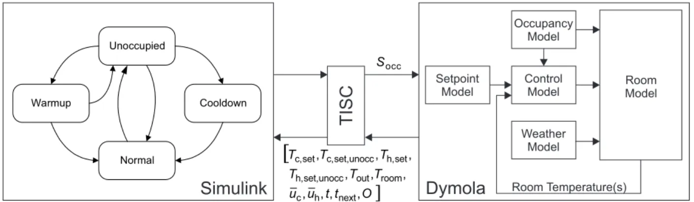
To compare models for predicting the return time from night setback, data are needed that relate return time to room air temperature, outdoor air temperature, and room heating or cooling demand at the beginning of the optimal start period, and the room air temperature at the end of the optimal start period. (Theoptimal start periodis the period of time between the beginning and end of the Warmup or Cooldown state. These states are introduced in the next paragraph.) Computer simulations were used to generate the data. The simulation platform consists of a Modelica building model implemented in Dymola, and the optimal start algorithm implemented as a Matlab function in Simulink. The Dymola and Simulink models run synchronously and exchange data through the middleware TISC (Kossel et al., 2006). Figure 1 illustrates the simulation platform and the data exchange between the simulation tools. At each time step the optimal start algorithm determines the state of operation (Unoccupied, Warmup, Cooldown or Normal) appropriate for the current time and conditions and passes a binary variableSoccto Dymola indicating whether the building model

should use occupied or unoccupied setpoints for room temperature control during the next time step. The building model executes using the appropriate room setpoints and then passes data back to the optimal start algorithm that are used to determineSoccfor the next time step. Included in these data are the occupied (Tc,set) and unoccupied (Tc,set,unocc)

cooling setpoints, the occupied (Th,set) and unoccupied (Th,set,unocc) heating setpoints, the room (Troom) and outdoor

(Tout) temperatures, and exponentially weighted moving averages (EWMAs) of the normalized room cooling (¯uc) and

heating (¯uh) demands. The data also include the current time (t), the time until the next occupied period (tnext), and the

occupancy status (O). The following sections provide more detailed descriptions of the building model and optimal start algorithm. Important factors influencing return time that are considered in this study are then described.

2.1 Description of the Building Model

The building model in Figure 1 consists of either a single-room or multi-room model interfaced to a control model, a weather model, an occupancy model, and models needed for data exchange (not shown). At each time step a setpoint model provides the room heating and cooling setpoints to the control model based on the value ofSocc. For the

multi-room model, a single multi-room was selected from the five controlled multi-rooms to be used in the optimal start algorithm. Thus, when the variableSoccchanges, indicating the setpoints for the representative room should be changed from unoccupied

Occupancy Model Setpoint

Model ControlModel Weather Model Room Model Room Temperature(s) Unoccupied Cooldown Warmup Normal

TISC

Dymola

Simulink





to occupied values (or from occupied to unoccupied), all the room setpoints are changed simultaneously.

The single-room model was adapted from the OneRoom_HVAC model distributed with the HumanComfort Library (Michaelsen & Eiden, 2009) and is modeled as a perimeter room on an intermediate floor of a multi-floor building. The multi-room model was adapted from the VAVReheat model distributed with the Buildings Library (Wetter et al., 2014) and consists of a core room coupled to four perimeter rooms. Collectively, the five rooms are modeled as an intermediate floor of a multi-floor building. Some of the heat transfer mechanisms in the room models are (Wetter et al., 2011; Michaelsen & Eiden, 2009): 1) transient heat conduction through multi-layered walls; 2) heat conduction and solar radiation transmitted through windows; 3) convection at interior and exterior surfaces of walls and windows; 4) solar radiation distribution within the room; and 5) infrared radiation exchange between surfaces in the room. The room models treat the air as well mixed. Individual rooms have a heat port that connects to the air volume of the room. In the simulations, the room temperature is controlled by adding a sensible convective heat flow to the air volume using this heat port. The air temperature of the individual room is input to a feedback controller (contained in the control model) to determine the sensible heat flow needed to maintain the room temperature within the limits defined by the current temperature setpoints. This sensible heat flow is the room heating (for positive values) or cooling (for negative values) demand.

2.2 Description of the Optimal Start Algorithm

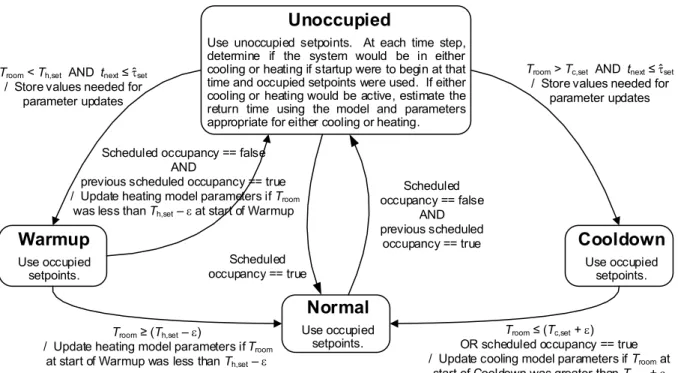
Figure 2 shows a detailed state transition diagram for the optimal start algorithm. As stated previously, there are four states: Unoccupied, Warmup, Cooldown, and Normal. During the Unoccupied state, unoccupied heating and cooling setpoints are used to control the room temperature. At each time step, the algorithm determines whether it is necessary to initiate either heating (Warmup) or cooling (Cooldown) using a model for predicting the return time for the current conditions. The model used for predicting the return timeˆτsetfor heating is given by

ˆτset=wh,1(Th,set−Troom)+wh,2¯uh+wh,3Tout (1)

wherewh,iare the heating model parameters and other variables are defined in the description of Figure 1. Equation 1

is used if the current value of the room temperatureTroomis less than the occupied heating setpointTh,set. The model

used for predicting the return time for cooling is given by

ˆτset=wc,1(Troom−Tc,set)+wc,2¯uc+wc,3Tout (2)

wherewc,i are the cooling model parameters. Equation 2 is used if the current value ofTroom is greater than the

occupied cooling setpoint Tc,set. The predicted return timeˆτset calculated from Equation 1 or 2 is compared with

the time remaining until the next occupied periodtnextand operation transitions to the appropriate state (Warmup or

Cooldown) if the time remaining until the next occupied period is less than or equal toˆτset. If the conditions for applying

Equations 1 and 2 are not satisfied, or iftnext>ˆτset, operation continues in the Unoccupied state unless the occupancy

schedule forces a transition to the Normal state. Prior to a transition to either the Warmup or Cooldown state, variables needed to update the parameters of the appropriate model must be stored.

The nomenclatureˆτsetin Equations 1 and 2 emphasizes that the initial prediction of the return time uses the occupied

heating setpoint as the target temperature during Warmup and the occupied cooling setpoint as the target temperature during Cooldown. The EWMA of the normalized heating demand¯uhis determined by calculating the EWMA of the

sensible heating divided by the maximum possible sensible heating (determined from sizing simulations). The EWMA of the normalized cooling demand¯ucis determined in a similar way. One-minute sampled values and a smoothing

constant of 0.05 are used to calculate the EWMAs.

During the Warmup state, the HVAC system is heating the room to raise the room temperature to the occupied heating setpoint temperature. If the room temperature rises above the target temperature (in this case the occupied heating setpoint minus an offsetε), control transitions to the Normal state. If the HVAC system has inadequate heating capacity, the room temperature may not reach the target temperature during the Warmup state. In this situation control transitions back to the Unoccupied state at the end of scheduled occupancy for that day. Prior to transitioning from the Warmup state, recursive least squares is used to update the heating model parameters provided the room temperature at the start of Warmup was less than the target temperature.

Unoccupied

Use unoccupied setpoints. At each time step, determine if the system would be in either cooling or heating if startup were to begin at that time and occupied setpoints were used. If either cooling or heating would be active, estimate the return time using the model and parameters appropriate for either cooling or heating.

Cooldown

Warmup

Normal

setpoints. OR scheduled occupancy == true Troom ≤ (Tc,set + e) / Update cooling model parameters if Troom at

start of Cooldown was greater than Tc,set + e

Troom ≥ (Th,set – e)

/ Update heating model parameters if Troom at start of Warmup was less than Th,set – e

Troom > Tc,set AND tnext ≤ tset / Store values needed for

parameter updates

Troom < Th,set AND tnext ≤ tset / Store values needed for

parameter updates Scheduled occupancy == false AND previous scheduled occupancy == true Scheduled occupancy == true Scheduled occupancy == false

AND

previous scheduled occupancy == true / Update heating model parameters if Troom

was less than Th,set – e at start of Warmup

ˆ ˆ

Figure 2: State transition diagram for optimal start algorithm

The offset parameterεis important for situations when the temperature asymptotically approaches the setpoint. Without the offset, the return time can include a period of time (perhaps significant in length) when the room temperature is nearly equal to the setpoint, but approaching it very slowly. If the model parameters are updated with this data point, the model will learn that it needs to start Warmup earlier (perhaps significantly earlier) for these conditions. The resultant impact on comfort will be minimal, but the impact on energy use could be significant.

During the Cooldown state, the HVAC system is cooling the room to lower the room temperature to the occupied cooling setpoint temperature. If the room temperature drops below the target temperature (in this case the occupied cooling setpoint plus an offsetε), or scheduled occupancy begins, control transitions to the Normal state. Prior to transitioning from the Cooldown state, recursive least squares is used to update the cooling model parameters provided the room temperature at the start of Cooldown was greater than the target temperature.

During the Normal state, the occupied heating and cooling setpoints are used to control the HVAC system. Control transitions to the Unoccupied state when the occupancy schedule changes to unoccupied.

At each time step, the optimal start algorithm uses internal variables and the inputs shown in Figure 1 to determine the state of operation and, based on the state, outputs the binary variableSoccindicating whether occupied or unoccupied

heating and cooling setpoints are to be used to control the room temperature. In addition, for each day that requires operation in either the Warmup or Cooldown state, the algorithm updates the appropriate model parameters using the actual return time and predictor variable values for that day. In particular, the room setpoint in Equations 1 and 2 is replaced by the actual room temperature at the end of the Warmup or Cooldown state.

2.3 Factors Affecting Return Time

The optimal start algorithm is intended for use in any building. As such, it is important to consider the main factors that are anticipated to affect the return time, and to assess the performance of the prediction models on a data set representative of these factors. The factors affecting return time considered in this study are climate, building thermal mass, room orientation (e.g., east facing, north facing), controller tuning, and unoccupied control strategy.

To study the influence of climate, simulations were performed using TMY3 weather data (Wilcox & Marion, 2008) for six U.S. cities representing a range of climatic conditions. The six cities considered are Baltimore, Boulder, Chicago, Miami, Phoenix, and Seattle.

The influence of the building mass on return time was studied by considering buildings with heavy and light construc-tions. For the simulations utilizing the room model from the Buildings Library, the heavy construction buildings have walls and floors that are the same as the Department of Energy (DoE) new construction reference large office building (Deru et al., 2010) for a particular location. The external wall layers of the heavy construction buildings consist of gypsum board, insulation, concrete, and stucco. The light construction buildings have walls and floors that are the same as the DoE reference medium office building for a particular location. The external wall layers of the light construction buildings consist of gypsum board, insulation and wood siding. The floors, ceilings and internal walls for the heavy and light construction buildings are identical.

The simulations utilizing the room model from the HumanComfort Library considered only a heavy construction build-ing. The external wall layer consists of concrete, insulation and a facade plate. The internal walls are hollow cinder blocks and the floor is concrete.

Room orientation can affect return time due to the potential for significant direct solar heat gain through east facing windows in the morning. For cooling, this will lengthen the return time compared to a day that is partly cloudy or cloudy, whereas for heating, it will reduce the return time. East and north facing rooms are included in the simulations. Controller tuning affects how aggressively the room temperature approaches the setpoint and therefore can influence return time. Cases with "well-tuned" proportional-integral (PI) controller parameters and other cases with controller parameters that result in "sluggish" and "very sluggish" controller behavior were simulated. The control loops of interest are used to regulate the sensible heating and cooling provided to the rooms. In the first step of the tuning process, relay auto-tuning was used to determine the ultimate period and ultimate gain for the rooms. From these values, the Tyreus-Luyben tuning relations (Seborg et al., 2004) were used to calculate the controller gains and integral times representative of "well-tuned" controllers. Sluggish and very sluggish controller behavior are obtained by dividing the well-tuned controller gain by five and ten, respectively.

The strategy used to control the room air temperature during unoccupied periods can impact the estimate of the return time because it affects the room temperature, a common input variable to return time models. Two different strategies are used in this study to control the heating and cooling during unoccupied periods, namely PI control and on-off control. Consider a situation in which the nighttime heating load on a room is sufficient to cause the room temperature to fall below the unoccupied heating setpoint. Assuming there is sufficient heating capacity, PI control will maintain the room air temperature at the unoccupied heating setpoint, whereas on-off control will cause the heating to cycle on and off and the room air temperature will rise and fall accordingly. During this period when the heating is cycling, the room air temperature could vary by several degrees. Because the model for predicting the return time commonly includes the room air temperature, the predicted return time could vary significantly over a 5-10 minute time period despite the fact that the load on the room has likely not changed in any significant way during this time.

Equipment sizing also affects return time. Since the HVAC equipment was not modeled in this study, sizing was performed by determining the maximum sensible convective heating and cooling inputs required to maintain the room temperature between its occupied setpoints for a one-year period (i.e., the building was assumed to be continuously occupied). The maximum sensible heating and cooling inputs for a given climate, building mass, and orientation are scaled by 120% and 140% to simulate equipment oversizing.

3. SUMMARY OF SIMULATION RESULTS

The results described in this section are based on data from 140 simulations. The simulations are one year in length and data were exchanged at one-minute intervals between the optimal start algorithm and building model. The multi-room model was occupied from 7 a.m. until 8 p.m. on weekdays and unoccupied on weekends. The single-room model was occupied from 6 a.m. until 6 p.m. on weekdays and unoccupied on weekends. Holidays were not simulated. All simulations include cooling data (days with return times of greater than 1 minute in the Cooldown state), while 104 of the simulations also had heating data (days with return times greater than 1 minute in the Warmup state). Each simulation took 3-6 hours to complete.

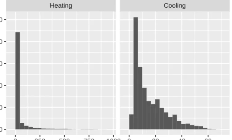
Histograms of the actual return times for heating and cooling are shown in Figure 3. Although difficult to see in Figure 3, the maximum return time for heating (888 minutes) is more than an order of magnitude larger than that for cooling (68 minutes). This is because the Cooldown state occurs early in the morning when the cooling load is relatively small compared to the peak load for which the equipment is sized, while the Warmup state coincides with the period when

the peak heating loads are experienced. It is evident that the histograms are heavily weighted toward shorter return times. For heating, 90% of the data have a return time less than 111 minutes, and for cooling, 90% of the data have a return time less than 34 minutes. The longest return times for both heating and cooling occur on Mondays after the building has been unoccupied and in night setback operation for the weekend.

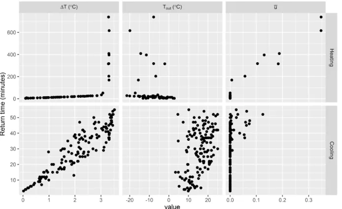
Plots of the return time versus candidate predictor variables for one simulation are shown in Figure 4 for both heating and cooling. The simulation case used the multi-room model, Chicago weather and wall construction, heavy mass, east orientation, very sluggish tuning, PI control during the unoccupied period and 20% oversizing. The plot label ΔT

corresponds to ΔTh=Tf−Tifor heating, whereTfandTiare the final and initial room temperatures during Warmup.

For cooling, ΔT=ΔTc=Ti−TfwhereTiandTfare the initial and final room temperatures during Cooldown. The plot

label¯ucorresponds to¯uhfor heating and¯ucfor cooling. The definitions of ΔTand¯ualso apply to tables that follow.

Although this is only one simulation out of more than 100, Figure 4 is illustrative when considering the results in the next section.

4. COMPARISON OF MODELS

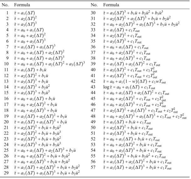
Table 1 lists the 57 models compared in this study. In Table 1,ai,biandciare the model parameters. The statistical

indices used for the model comparison and the results of that comparison are presented next.

4.1 Statistical Indices for Model Comparison

Results of the model comparison are reported in terms of two statistical indices. The root mean square of the prediction errors compares the actual and predicted return times for a single simulation and a single model and is given by

RMSPEm,s= ¿ Á Á Á Á À n ∑ i=1( τi−ˆτi,₋i)2 n (3)

whereτiis the actual return time for observationi,ˆτi,−iis the predicted return time for observationi,nis the number

of return times for a simulation, and subscriptssandmcorrespond to a particular simulation case and a particular model. ˆτi,−iis determined by removing observationifrom the data set, performing a regression with the remaining

observations, and using the parameter estimates to predict the return time for observationi. This procedure is called cross-validation with one sample left out. To summarize the performance of a model, the average RMSPE for each model over all simulations is determined from

Heating Cooling 0 1000 2000 3000 4000 5000 0 250 500 750 1000 0 20 40 60

Return time (minutes)

count

Figure 4: Actual return time versus candidate predictor variables for a single simulation RMSPEm= S ∑ s=1 RMSPEm,s S (4)

whereSis the total number of simulations. For each simulation, the difference between the root mean square of the prediction errors for model mand the minimum root mean square of the prediction errors for all models is given by

δm,s=RMSPEm,s− min

m=1 to 57(RMSPEm,s) (5)

Thus,δm,srepresents the performance of a particular model for a particular simulation relative to the best performing

model for that simulation. For each model, the worst case relative performance across all simulations is given by

δm,max= max

s=1 toS(δm,s) (6)

The statisticδm,maxcan help identify models that have poor performance on one or more simulations despite having

good performance on average. All other criteria being equal, preference in the model selection will be given to the model with the smallest value ofδm,max.

4.2 RESULTS

The top heating models based on their performance over all simulations are compared in Table 2. Each model in Table 2 has the lowest value of RMSPEmamong a subset of models from Table 1. For example, among the models with three

Table 1: Models compared for estimating return time from night setback

No. Formula No. Formula

1 ˆτ=a1(ΔT) 30 ˆτ=a3(ΔT)3+b1¯u+b2¯u2+b3¯u3 2 ˆτ=a2(ΔT)2 31 ˆτ=a2(ΔT)2+a3(ΔT)3+b1¯u+b2¯u2 3 ˆτ=a3(ΔT)3 32 ˆτ=a0+a2(ΔT)2+a3(ΔT)3+b1¯u+b2¯u2 4 ˆτ=a0+a1(ΔT) 33 ˆτ=a1(ΔT)+c1Tout 5 ˆτ=a0+a2(ΔT)2 34 ˆτ=a2(ΔT)2+c1Tout 6 ˆτ=a0+a3(ΔT)3 35 ˆτ=a3(ΔT)3+c1Tout 7 ˆτ=a1(ΔT)+a3(ΔT)3 36 ˆτ=a0+a1(ΔT)+c1Tout 8 ˆτ=a0+a1(ΔT)+a2(ΔT)2 37 ˆτ=a0+a2(ΔT)2+c1Tout 9 ˆτ=a0+a1(ΔT)+a3(ΔT)3 38 ˆτ=a0+a3(ΔT)3+c1Tout 10 ˆτ=a0+a1(ΔT)+a2(ΔT)2+a3(ΔT)3 39 ˆτ=a1(ΔT)+a2(ΔT)2+c1Tout 11 ˆτ=a1(ΔT)+b1¯u 40 ˆτ=a2(ΔT)2+c1Tout+c2T2out 12 ˆτ=a2(ΔT)2+b1¯u 41 ˆτ=a3(ΔT)3+c1Tout+c2T2out 13 ˆτ=a3(ΔT)3+b1¯u 42 ˆτ=a0+a1(1−w)(ΔT)+c1wTout 14 ˆτ=a3(ΔT)3+b2¯u2 43 logˆτ=a0+a1(ΔT)+c1Tout 15 ˆτ=a3(ΔT)3+b3¯u3 44 ˆτ=a0+a1(ΔT)+a2(ΔT)2+c1Tout 16 ˆτ=a0+a1(ΔT)+b1¯u 45 ˆτ=a0+a2(ΔT)2+c1Tout+c2T2out 17 ˆτ=a0+a2(ΔT)2+b1¯u 46 ˆτ=a0+a3(ΔT)3+c1Tout+c2T2out 18 ˆτ=a0+a3(ΔT)3+b1¯u 47 ˆτ=a2(ΔT)2+a3(ΔT)3+c1Tout+c2T2out 19 ˆτ=a1(ΔT)+a2(ΔT)2+b1¯u 48 ˆτ=a0+a2(ΔT)2+a3(ΔT)3+c1Tout+c2T2out 20 ˆτ=a1(ΔT)+a3(ΔT)3+b1¯u 49 ˆτ=a1(ΔT)+b1¯u+c1Tout 21 ˆτ=a2(ΔT)2+b1¯u+b2¯u2 50 ˆτ=a2(ΔT)2+b1¯u+c1Tout 22 ˆτ=a2(ΔT)2+b1¯u+b3¯u3 51 ˆτ=a3(ΔT)3+b1¯u+c1Tout 23 ˆτ=a3(ΔT)3+b1¯u+b2¯u2 52 ˆτ=a0+a1(ΔT)+b1¯u+c1Tout 24 ˆτ=a3(ΔT)3+b1¯u+b3¯u3 53 ˆτ=a0+a2(ΔT)2+b1¯u+c1Tout 25 ˆτ=a0+a1(ΔT)+a2(ΔT)2+b1u¯ 54 ˆτ=a0+a3(ΔT)3+b1¯u+c1Tout 26 ˆτ=a0+a2(ΔT)2+b1¯u+b2¯u2 55 ˆτ=a3(ΔT)3+b1¯u+b2¯u2+c1Tout 27 ˆτ=a0+a3(ΔT)3+b1¯u+b2¯u2 56 ˆτ=a1(ΔT)+a2(ΔT)2+b1¯u+c1Tout 28 ˆτ=a1(ΔT)+a2(ΔT)2+b1¯u+b2¯u2 57 ˆτ=a1(ΔT)+a3(ΔT)3+b1¯u+c1Tout 29 ˆτ=a1(ΔT)+a3(ΔT)3+b1¯u+b2¯u2

Among the models with one or two parameters, model 13 is clearly superior based on the statistical measures in Table 2. Performance exceeding that of model 13 can be achieved (e.g., by models 24, 51, 27, 55, and 32), but the improvement comes at a cost of one or more additional parameters and does not appear to be sufficient to justify a more complex model. It is interesting to note that models of the formˆτ =f(ΔTh,Tout)perform poorly compared with the

best performing models of the formˆτ=f(ΔTh,¯uh). For instance, model 13 is far superior to model 35. Furthermore,

the top six models in Table 2 use¯uhas an input, but only two of the six useTout. Although it is only one simulation, it

is apparent from Figure 4 that the return time for the heating data are better correlated to¯uhthanTout. Based on these

results, model 13 is recommended for predicting the return time from night setback when heating is needed.

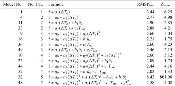
The top cooling models based on their performance over all simulations are compared in Table 3. Note the prediction errors quantified by RMSPEmare significantly smaller than those for heating in Table 2. This is expected because the

return times for cooling are significantly shorter than those for heating.

From Table 3 it can be seen that all the models perform well, with the exception of model 32. For model 32 there is a single simulation for which the RMSPE is 862.5 minutes. This results in the relatively large value of RMSPEm, and

the extreme value ofδm,max. Among the cooling models with one or two parameters, the performances of models 4, 11,

and 33 are nearly the same. Model 11 has a slightly larger value of RMSPEmthan the other two models, but a smaller

value ofδm,maxand is recommended over the other two models for this reason. Better performance can be achieved

with models having more parameters, but the additional complexity is not justified based on these results. Thus, model 11 is recommended for use for predicting the return time from night setback when cooling is needed.

Table 2: Top performing heating models for different numbers of parameters and inputs (Results in minutes)

Model No. No. Par. Formula RMSPEm δm,max

3 1 ˆτ=a3(ΔTh)3 66.43 141.15 7 2 ˆτ=a1(ΔTh)+a3(ΔTh)3 65.05 142.28 13 2 ˆτ=a3(ΔTh)3+b1¯uh 36.06 80.26 35 2 ˆτ=a3(ΔTh)3+c1Tout 65.79 142.40 9 3 ˆτ=a0+a1(ΔTh)+a3(ΔTh)3 64.24 142.62 24 3 ˆτ=a3(ΔTh)3+b1¯uh+b3¯u3h 35.29 80.26 38 3 ˆτ=a0+a3(ΔTh)3+c1Tout 65.53 142.81 51 3 ˆτ=a3(ΔTh)3+b1¯uh+c1Tout 35.37 75.56 10 4 ˆτ=a0+a1(ΔTh)+a2(ΔTh)2+a3(ΔTh)3 63.62 146.29 27 4 ˆτ=a0+a3(ΔTh)3+b1¯uh+b2¯u2h 34.89 79.63 47 4 ˆτ=a2(ΔTh)2+a3(ΔTh)3+c1Tout+c2T2out 65.64 145.00 55 4 ˆτ=a3(ΔTh)3+b1¯uh+b2¯u2h+c1Tout 34.79 75.56 32 5 ˆτ=a0+a2(ΔTh)2+a3(ΔTh)3+b1¯uh+b2¯u2h 35.81 61.19 48 5 ˆτ=a0+a2(ΔTh)2+a3(ΔTh)3+c1Tout+c2T2out 65.16 146.48

Table 3: Top performing cooling models for different numbers of parameters and inputs (Results in minutes)

Model No. No. Par. Formula RMSPEm δm,max

1 1 ˆτ=a1(ΔTc) 3.44 6.25 4 2 ˆτ=a0+a1(ΔTc) 2.77 4.98 11 2 ˆτ=a1(ΔTc)+b1¯uc 2.90 2.85 33 2 ˆτ=a1(ΔTc)+c1Tout 2.88 4.21 9 3 ˆτ=a0+a1(ΔTc)+a3(ΔTc)3 2.60 5.04 16 3 ˆτ=a0+a1(ΔTc)+b1¯uc 2.21 1.75 36 3 ˆτ=a0+a1(ΔTc)+c1Tout 2.60 4.23 49 3 ˆτ=a1(ΔTc)+b1¯uc+c1Tout 2.46 2.15 10 4 ˆτ=a0+a1(ΔTc)+a2(ΔTc)2+a3(ΔTc)3 2.60 5.12 25 4 ˆτ=a0+a1(ΔTc)+a2(ΔTc)2+b1¯uc 2.09 1.74 44 4 ˆτ=a0+a1(ΔTc)+a2(ΔTc)2+c1Tout 2.44 4.16 52 4 ˆτ=a0+a1(ΔTc)+b1¯uc+c1Tout 2.02 1.33 32 5 ˆτ=a0+a2(ΔTc)2+a3(ΔTc)3+b1¯uc+b2¯u2c 8.43 861.90 48 5 ˆτ=a0+a2(ΔTc)2+a3(ΔTc)3+c1Tout+c2T2out 2.58 4.08

To summarize, model 13 is recommended for predicting the return time from night setback for heating and is given by

ˆτh=wh,1(ΔTh)3+wh,2¯uh (7)

Model 11 is recommended for predicting the return time from night setback for cooling and is given by

ˆτc=wc,1(ΔTc)+wc,2¯uc (8)

Although the models recommended for predicting the return time for heating and cooling do not use the outdoor air temperature as a predictor variable, the outdoor temperature affects the normalized heating and cooling demand and, therefore, is indirectly included. By including an EWMA of the normalized heating and cooling demand in the models, the recent history of the heating and cooling in the room, including intermittent heating and cooling required to keep the room temperature within the bounds of the unoccupied setpoints, can be captured.

5. CONCLUSIONS AND FUTURE WORK

The performance of 57 models for predicting return time from night setback was compared using simulation data reflecting the influence of climate, building mass, controller tuning, room orientation, and the unoccupied control strategy. The return times for heating were significantly longer than those for cooling and separate models are recom-mended for the two cases. In each case, a two-parameter model is recomrecom-mended that uses the room air temperature and an EWMA of the normalized heating or cooling demand as predictor variables. The outdoor air temperature, a common input for predicting return time, is not used in the recommended models, but is indirectly included through its influence on the heating and cooling demands.

Future work will entail testing the preferred models using the same simulation test bed described here and will con-sider the energy and comfort tradeoffs associated with practical implementation issues such as limiting the maximum allowable return time and changing the unoccupied heating and cooling setpoints.

REFERENCES

Birtles, A. B., & John, R. W. (1985). A new optimum start control algorithm.Building Services Engineering Research and Technology,6(3), 117-122.

Deru, M., Field, K., Studer, D., Benne, K., Griffith, B., Torcellini, P., … Crawley, D. (2010). U.S. Department of Energy commercial reference building models of the national building stock (Tech. Rep.). Washington, DC: U.S. Department of Energy, Energy Efficiency and Renewable Energy, Office of Building Technologies. Fraisse, G., Virgone, J., & Yezou, R. (1999). A numerical comparison of different methods for optimizing

heating-restart time in intermittently occupied buildings. Applied Energy,62, 125-140.

John, R. W., & Salvidge, A. C. (1986). The BRE low energy office - five years on. Building Services Engineering Research and Technology,7(4), 121-128.

Kossel, R., Tegethoff, W., Bodmann, M., & Lemke, N. (2006). Simulation of complex systems using Modelica and tool coupling. InProc. of the 5th International Modelica Conference, Vienna, Austria(p. 485-490).

Levermore, G. J. (2000). Building energy management systems: Applications to low-energy HVAC and natural ventilation control. London: E & FN Spon.

Michaelsen, B., & Eiden, J. (2009). HumanComfort Modelica-library: Thermal comfort in building and mobile applications. InProc. of the 7th International Modelica Conference, Como, Italy(p. 403-412).

Seborg, D., Edgar, T. F., & Mellichamp, D. A. (2004).Process dynamics and control: Second edition. Hoboken, NJ: John Wiley & Sons, Inc.

Seem, J. E., Armstrong, P. R., & Hancock, C. E. (1989). Algorithms for predicting recovery time from night setback.

ASHRAE Transactions,95, 439-446.

Vrecko, D., Vodopivec, N., & Strmcnik, S. (2009). An algorithm for calculating the optimal reference temperature in buildings. Energy and Buildings,41, 182-189.

Wetter, M., Zuo, W., Nouidui, T., & Pang, X. (2014). Modelica Buildings library. Journal of Building Performance Simulation,7(4), 253-270.

Wetter, M., Zuo, W., & Nouidui, T. S. (2011). Modeling of heat transfer in rooms in the Modelica "Buildings" library. InProc. of the 12th Conference of International Building Performance Simulation Association, Sydney, Australia

(p. 1096-1103).

Wilcox, S., & Marion, W. (2008).Users manual for TMY3 data sets(Tech. Rep. No. NREL/TP- 581-43156). Golden, CO: National Renewable Energy Laboratory.

Yang, I., Yeo, M., & Kim, K. (2003). Application of artificial neural network to predict the optimal start time for heating system in building. Energy Conversion and Management,44, 2791-2809.

ACKNOWLEDGMENT

The authors would like to thank Tim Salsbury for his contribution to the discussion of the model selection proce-dure.