Calhoun: The NPS Institutional Archive
Faculty and Researcher Publications Faculty and Researcher Publications
2012-05
Analysis of multi-state systems with
multi-state components using EVMDDs
Nagayama, Shinobu
S. Nagayama, T. Sasao, and J. T. Butler,"Analysis of multi-state systems with multi-state
components using EVMDDs," International Symposium on Multiple-Valued Logic (ISMVL-2012),
Victoria, Canada, May 14-16, 2012, pp.122-127.
Analysis of Multi-State Systems with Multi-State Components Using EVMDDs
Shinobu Nagayama∗ Tsutomu Sasao† Jon T. Butler‡
∗Dept. of Computer and Network Eng., Hiroshima City University, Hiroshima, JAPAN †Dept. of Computer Science and Electronics, Kyushu Institute of Technology, Iizuka, JAPAN
‡Dept. of Electr. and Comp. Eng., Naval Postgraduate School, Monterey, CA USA
Abstract—This paper proposes a new analysis method of state systems with state components using multi-valued decision diagrams (MDDs). The multi-state systems with multi-state components can be considered as multi-valued func-tions, called structure functions. Since the structure functions are usually monotone increasing functions, they can be rep-resented compactly using edge-valued MDDs (EVMDDs). This paper proposes an efficient analysis method using EVMDDs. It shows that by using EVMDDs, the structure functions can be represented more compactly than existing methods using ordinary MDDs, and systems can be analyzed with comparable computation time.
Keywords-multi-state systems with multi-state components; fault tolerant systems; structure functions; system analysis based on decision diagrams; EVMDDs.
I. INTRODUCTION
In recent years, various systems such as computer server systems, telecommunication systems, water, gas, and elec-tricity distribution systems, become tolerant to faults and errors. Even if a fault occurs, these systems still keep on working with an acceptable or degraded performance level. Thus, these systems cannot be modeled by two states: work-ing and failure. In addition, with the advance of technology, each component in a system also becomes fault tolerant. To model such systems, a multi-state system with multi-state components are often used [11], [14], [16].
Fault tolerance is usually achieved by multiplexing com-ponents in a system. However, multiplexing noncritical components to design a fault tolerant system is inefficient and not cost effective. Also, if critical components are not sufficiently tolerant to faults, fault tolerance of the system is not sufficient. Thus, identifying which components are critical to achieve fault tolerance of the system, and mul-tiplexing them are important, especially for safety-critical systems such as flight control systems and nuclear power plant monitoring systems [2].
To identify critical components and system weaknesses, analyzing multi-state systems by various assessment mea-sures is required [11]. Among them, assessing the proba-bility of each state of a multi-state system is essential to the design of a dependable fault tolerant system [14], [16]. Various methods to analyze multi-state systems efficiently have been proposed. Many existing methods are based on the Markov model [3]. However, they are impractical for
a large multi-state system, since their time complexity is
O(m3n), where m is the number of states, and n is the number of components in a multi-state system [2]. To analyze large multi-state systems efficiently, methods based on binary decision diagrams (BDDs) [1], [2], [4], [16] and multi-valued decision diagrams (MDDs) [6], [13], [14] have attracted much attention.
Since multi-state systems with multi-state components can be considered as multi-valued functions, called structure functions, they can be represented by BDDs and MDDs. Probabilities of states can be computed using BDDs and MDDs with the time complexity proportional to the number of nodes in a decision diagram. BDDs represent structure functions by converting multi-valued variables and function values into binary vectors using one-hot encoding [16]. By using BDDs, various analysis methods well-established for binary-state systems can be directly applied to multi-state systems. However, converting into binary vectors produces many binary variables and many binary functions, and results in large BDDs. Thus, use of MDDs is more natural and more promising for larger multi-state systems.
For recent large and complex multi-state systems, how-ever, decision diagrams that represent systems more com-pactly are desired. Since structure functions are usually monotone increasing [13], they can be represented com-pactly using edge-valued MDDs (EVMDDs) [10]. How-ever, analysis of multi-state systems using EVMDDs is not straightforward. As far as we know, an analysis method using EVMDDs has never been reported. Thus, in this paper, we propose an efficient analysis method using EVMDDs.
This paper is organized as follows: Section II defines multi-state systems, and EVMDDs. Section III shows repre-sentations of structure functions using MDDs and EVMDDs, and in Section IV, we propose an analysis method using EVMDDs. Experimental results are shown in Section V.
II. PRELIMINARIES
This section defines multi-state systems, structure func-tions, and MDDs to represent structure functions.
A. Multi-State Systems and Structure Functions
Definition 1: Amulti-state systemis a model of systems, which represents performance, capacity, or reliability levels 2012 IEEE 42nd International Symposium on Multiple-Valued Logic
S
T
1
x
x
23
x
x
4(a) Multi-state system.
x1 x2 x3 x4 f 0 0 0 0 0 0 0 0 1 0 0 0 0 2 0 0 0 1 0 0 0 0 1 1 1 .. . ... 2 2 2 2 5 (b) Structure function. Figure 1. Multi-state system for network flow and its structure function.
of the systems as states. It usually has more than two states. When components in a system are modeled as well, it is called amulti-state system with multi-state components. In this paper, it is simply called multi-state system.
Definition 2: A state of a multi-state system depends only on states of components in the system. The system with n
components can be considered as a multi-valued function
f(x1,x2,...,xn) : R1×R2×...×Rn →M, where each xi
represents a component withristates,Ri={0,1,...,ri−1}
is a set of the states, andM={0,1,...,m−1} is a set of them system states. This multi-valued function is called a structure functionof the multi-state system.
Definition 3: A multi-valued function f(x1,x2,...,xn)is
amonotone increasing function iff for anyxi,
f(x1,x2,...,xi−1,α,xi+1,...,xn)
≤ f(x1,x2,...,xi−1,β,xi+1,...,xn),
whereα,β∈Ri, andα≤β.
In many applications, states of a system and its compo-nents are totally ordered, and deterioration of a component in the system affects deterioration of the whole system. Thus, structure functions usually become monotone increasing functions by assigning a value to each state in ascending order (i.e. the worst state is 0 and the best state ism−1 or
ri−1).
Example 1: Fig. 1(a) shows a multi-state system for net-work flow such as water, gas, and electricity distribution systems. In this figure, each edgexi has three states which
correspond to transmission capacities: 0 unit (disconnected), 3 units (deteriorated), and 5 units (fully transmittable). And, the system has six states which correspond to the maximum number of units that the target node T can receive from the source node S: 0, 3, 5, 6, 8, and 10.
By assigning six values (0, 1, 2, 3, 4, and 5) to these states in ascending order, we obtain the 6-valued structure function f shown in Fig. 1(b). This is a monotone increasing
function. (End of Example)
x4 0 1 2 x4 x3 x2 x2 x1 1 0 2 1 2 0 1 2 0 0 1 2 1 0 20 1 2 x4 1 3 4 x4 x3 0 1 2 1 0 20 1 2 x4 2 4 5 x4 x3 0 1 2 1 0 20 1 2 v1 v2 v3 v4 v5
Figure 2. MDD for the structure function.
2 x4 0 x4 x3 x2 x2 x1 1 0 2 1 2 01 2 0 0 1 2 1 0 2 0 1 2 x3 0 1 2 1 1 1 3 x4 x4 1 0 2 0 1 2 2 2 2 1 1 1 2
Figure 3. EVMDD for the structure function.
B. Multi-Valued Decision Diagrams
Definition 4: Amulti-valued decision diagram (MDD)
is a rooted DAG representing a multi-valued function f. The MDD is obtained by repeatedly applying the Shannon expansion to the multi-valued function [5]. It consists of non-terminal nodes representing sub-functions obtained from f
by assigning values to certain variables. It also has terminal nodes representing function values. Each non-terminal node has multiple outgoing edges that correspond to the values of multi-valued variable. The MDD is ordered; i.e., the order of variables along any path from the root node to a terminal node is the same. When an MDD represents a function for which multi-valued variables have different domains, it is a heterogeneous MDD [8]. In the following, a heterogeneous MDD is also denoted by the MDD.
Definition 5: An edge-valued MDD (EVMDD) [10] is
an extension of the MDD, and represents a multi-valued function. It consists of one terminal node representing 0 and non-terminal nodes with edges having integer weights; 0-edges always have zero weights. In an EVMDD, the function value is represented as a sum of weights for edges traversed from the root node to the terminal node.
Example 2: Fig. 2 and Fig. 3 show an ordinary MDD
and an EVMDD for the structure function of Example 1. (End of Example) III. MDDS ANDEVMDDS FORSTRUCTUREFUNCTIONS This section derives upper bounds on the number of nodes in an MDD and an EVMDD for a structure function. For simplicity, in the following theorems, we assume that all components xi in a system have the same number r of
states (i.e., all variablesxihave the same domain). However,
generalization to a case where all variablesxi have different
domains is straightforward.
Theorem 1: For a structure function, the number of nodes in an MDD is at most
rn−l−1
r−1 +m
rl
,
wherel is the largest integer satisfyingrn−l≥mrl,mis the
number of system states, n is the number of components, andr is the number of component states.
(Proof) See Appendix.
Theorem 1 shows that the upper bound for an MDD depends only on m, n, and r. It is independent of mono-tonicity of structure functions. However, in many applica-tions, structure functions are usually monotone increasing. Thus, decision diagrams suitable for monotone functions are preferable. Since EVMDDs can represent monotone functions compactly, EVMDDs are preferable for many monotone structure functions.
Definition 6: Let N0 be the set of nonnegative integers,
and let p be an integer. An integer function f(X):N0→Z
such that 0≤f(X+1)−f(X)≤pand f(0) =0 is anMp -monotone increasing functiononN0, whereZis the set of
integers. That is, an Mp-monotone increasing function f(X)
satisfies f(0) =0, and the increment ofX by one increases the value of f(X)by at most p.
A monotone multi-valued function can be converted into an Mp-monotone increasing function by considering the set of multi-valued variablesxi as anr-valued vector:
X= (xn,xn−1,...,x1)r,
and EVMDDs for monotone multi-valued functions have the same complexity as EVMDDs for Mp-monotone increasing functions [10]. Thus, we derive an upper bound of an EVMDD for an Mp-monotone increasing function in the following:
Theorem 2: For an Mp-monotone increasing function converted from a multi-valued function, the number of nodes in an EVMDD is at most rn−l−1 r−1 + l
∑
i=1 (p+1)ri−1−l,where l is the largest integer satisfying rn−l≥(p+1)rl−1, andnis the number of variables in the original multi-valued function.
(Proof) This is the straightforward generalization of the theorem for edge-valued binary decision diagrams (EVB-DDs) [9] (i.e., r=2). Thus, we can also extend the proof for EVBDDs to EVMDDs trivially.
Theorem 2 shows that the upper bound for an EVMDD depends on the value of p, not on the number of system statesm. Thus, even if mis large, EVMDDs have a small number of nodes when the value ofpis small. In the future, systems will become more complex, and thus,mwill become larger. For such systems, MDDs require many nodes. On the other hand, EVMDDs can represent even such systems compactly if the value of pis small.
IV. ANALYSISMETHODSUSINGMDDS ANDEVMDDS This section formulates a problem of system analysis, and then proposes an algorithm to solve the problem using EVMDDs.
Definition 7: The probability that a structure function
f has the value s is denoted by Ps(f = s), where s∈
{0,1,...,m−1}. The probability that a componentxihas the
valuecis denoted byPc(xi=c), wherec∈ {0,1,...,ri−1}.
Problem 1: Given a structure function f of a multi-state system and the probability of each state of each component in the system Pc(xi=c), compute the probability of each
state of the multi-state systemPs(f =s).
In this problem, we assume that all components are independent of each other. That is, each state of a component appears independently of the states of other components.
A. Analysis Method Using MDDs
Problem 1 can be solved efficiently usingnode traversing probabilitiesin an MDD that are introduced to compute the average path length on an MDD [7].
Definition 8: In an MDD, a sequence of edges and nodes leading from the root node to a terminal node is apath. The node traversing probability, denoted by NT P(vi), is the
probability that an assignment of values to variables selects a path that includes the nodevi.
Since terminal nodes of an MDD for a structure function represent system states, node traversing probabilities of terminal nodes correspond to the probabilities of system states. The node traversing probabilities can be computed by visiting each node only once in the breadth first order from the root node. Thus, the time complexity of this analysis method is O(NM), where NM is the number of nodes in
an MDD. Other existing methods whose time complexity is
O(NM)also analyze multi-state systems in a similar way [6],
[13], [14].
Example 3: Let us compute node traversing probabil-ities for the MDD in Fig. 2. In this example, we as-sume that all states of each component occur with the same probability 1/3. First, we have NT P(v1) = 1 for
the root node v1 since the root node occurs in all
Input: An EVMDD for a structure function of a multi-state system, and the probability of each state of each component in the systemPc(xi=c).
Output: Probability of each state of the multi-state system Ps(f =s).
Step: The following procedures are applied to each node recursively from the root node.
1. If a nodevhas been already visited, then return probabilities for the sub-function fv that have been already
computed. Else, go to the next step.
2. If the nodevis the terminal nodeT, then return the probability for the constant zero function:Ps(fT=0) =1.
Else, go to the next step.
3. Visit all child nodes ui ofv, and obtain probabilities for the sub-functions fui represented byui.
4. Multiply the obtained probabilities for a sub-function Ps(fui=s)by the probability that the componentxi selects the sub-functionPc(xi=c).
5. Each function value fui=sat each child nodeui becomes a function value fv=s+eiat the nodevbecause of its edge value ei. Thus, the probabilities Ps(fui =s)×Pc(xi=c) obtained by the step 4 are added to
Ps(fv=s+ei), and they are summed up (merged) in each function value atv.
6. Return the merged probabilities to a parent node.
Figure 4. Proposed analysis algorithm using EVMDDs.
NT P(v3) =NT P(v1)×1/3 in a breadth first order.
Sim-ilarly, NT P(v4) =NT P(v1)/3+NT P(v2)/3+NT P(v3)/3,
NT P(v5) = 2NT P(v2)/3+NT P(v3)/3, and finally we
have the node traversing probabilities of terminal nodes:
NT P(0) = 25/81, NT P(1) = 10/27, NT P(2) = 10/81,
NT P(3) = 1/9, NT P(4) = 2/27, and NT P(5) = 1/81. (End of Example)
B. Analysis Method Using EVMDDs
In an EVMDD, a function value is represented by a sum of edge values, rather than a terminal node. Thus, we cannot solve Problem 1 using only node traversing probabilities, and another analysis method is needed.
Fig. 4 shows the proposed analysis algorithm. This al-gorithm visits each node only once in depth first order starting from the root node, and analyzes a sub-function represented by each node recursively. Probabilities for a function represented by a node can be computed by merging probabilities for sub-functions represented by its child nodes. Thus, the algorithm shown in Fig. 4 can compute the probability of each state of a multi-state system correctly and efficiently. Since the algorithm visits each node only once, its time complexity isO(NE), whereNE is the number
of nodes in an EVMDD.
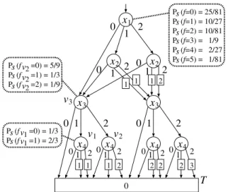
Example 4: Let us compute the probability of each state of the multi-state system using the EVMDD in Fig. 3. As with the previous example, we assume that all states of each component appear in the same probability 1/3. First, we have Ps(fT =0) =1 at the terminal node T. Then, we
compute probabilities for a sub-function at the node v1.
Since this node has two edges pointing to T whose values are 1, we have Ps(fT=0)×Pc(x4=1) =1/3, Ps(fT=0)×Pc(x4=2) =1/3,and thus, 2 x4 0 x4 x3 x2 x2 x1 1 0 2 1 2 0 1 2 0 0 1 2 1 0 2 0 1 2 x3 0 1 2 1 1 1 3 x4 x4 1 0 2 0 1 2 2 2 2 1 1 1 2 v1 v2 v3 P (f =0) = 1/3 P (f =1) = 2/3 P (f =0) = 5/9 P (f =1) = 1/3 P (f =2) = 1/9 P (f=0) = 25/81 P (f=1) = 10/27 P (f=2) = 10/81 P (f=3) = 1/9 P (f=4) = 2/27 P (f=5) = 1/81 s s v v11 T s s s s s s s s s v2 v2 v2
Figure 5. Analysis of the multi-state system using EVMDD.
Ps(fv1 =0+1) =Ps(fT =0)×Pc(x4=1)
+Ps(fT=0)×Pc(x4=2) =2/3
Similarly, at the nodev2, we have
Ps(fv2=0+0) =Ps(fT =0)×Pc(x4=0) =1/3, Ps(fv2=0+1) =Ps(fT =0)×Pc(x4=1) =1/3,and Ps(fv2=0+2) =Ps(fT =0)×Pc(x4=2) =1/3.
At v3, the probabilities at the terminal node, v1, and v2
are multiplied by 1/3, and are summed up. Thus, we have
Ps(fv3=0) =5/9,Ps(fv3=1) =1/3, andPs(fv3=2) =1/9.
By performing the same computation at each node in the depth first order, we have the following at the root node:
Ps(f =0) =25/81,Ps(f =1) =10/27,Ps(f=2) =10/81,
Ps(f =3) =1/9,Ps(f =4) =2/27, andPs(f =5) =1/81.
Table I
MDDS ANDEVMDDS FORm-STATE SYSTEMS WITHn3-STATE COMPONENTS. n m Number of nodes Computation time (μsec.)
MDD EVMDD Ratio MDD EVMDD Ratio
5 3 12 10 83% 0.30 1.20 406% 5 10 36 18 50% 1.10 2.52 230% 10 3 17 15 88% 0.52 1.85 355% 10 10 77 57 74% 2.83 7.84 277% 10 100 599 265 44% 26.41 49.27 187% 10 1,000 4,201 907 22% 231.10 317.79 138% 15 3 32 30 94% 1.16 3.72 320% 15 10 120 105 88% 4.94 14.07 285% 15 100 1,098 708 64% 59.43 110.72 186% 15 1,000 9,010 3,362 37% 589.10 744.59 126% 15 10,000 70,140 11,474 16% 4,705.00 4,701.00 100% 15 100,000 495,224 62,759 13% 65,303.00 60,901.00 93% n: Number of 3-state components. m: Number of states for systems. Ratio: EVMDD / MDD×100 (%)
The computation time is an average time obtained by running the same computation a million times, and dividing its total time by a million.
Note that these are consistent with the results obtained by MDDs in Example 3. (End of Example) When a structure function is monotone increasing, the number of nodes in an EVMDD NE is smaller than for
non-monotone increasing functions, and thus, computation time is shorter. Of course, the proposed method can be applied to nonmonotonic structure functions used in some applications [14], [16] as well.
V. EXPERIMENTALRESULTS
To show the effectiveness of the proposed method, we used various structure functions. Unfortunately, however, benchmark structure functions of multi-state systems were unavailable. Since structure functions are usually monotone increasing, we randomly generated M1-monotone increas-ing functions, and used them as structure functions for experiments in this paper. The analysis algorithms based on MDDs and EVMDDs are implemented using the follow-ing computer environment: CPU: Intel Core2 Quad Q6600 2.4GHz, memory: 4GB, OS: CentOS 5.7, and C-compiler: gcc -O2 (version 4.1.2). Table I shows the experimental results for randomly generated m-state systems with n 3-state components.
From this table, we can see that EVMDDs have fewer nodes than MDDs for all the functions. Especially, as the number of states m becomes larger, EVMDDs are much smaller than MDDs. We expect that systems will become more complex in the future, and thatmwould become larger. Thus, EVMDDs whose size is independent of the number of states are more promising. However, when m is very small, MDDs are better, since they are small enough and computation time is shorter. In Table I, when m=3, only two terminal nodes are reduced in EVMDDs. Thus, using EVMDDs for such systems is not effective.
As for computation time, the proposed method using EVMDDs is comparable to methods using MDDs.
There-fore, we can say that EVMDDs are suitable for compact representation and efficient analysis ofmany-state systems.
VI. CONCLUSION ANDCOMMENTS
This paper proposes an efficient analysis method of multi-state systems using EVMDDs. The proposed analysis method is somewhat more complicated than existing meth-ods using ordinary MDDs because a state of the system is represented by a sum of edge values. However, actual computation time of the proposed method is comparable to methods using MDDs since the time complexity is asymp-totically proportional to the number of nodes in an EVMDD, and EVMDDs have fewer nodes than MDDs. Especially, for systems with many states, the proposed method is effective because EVMDDs are much smaller than MDDs. Even if structure functions are not monotone, EVMDDs are not larger than MDDs. Thus, the proposed method is effective for a wide range of structure functions.
In this paper, we used randomly generated M1-monotone increasing functions for our experiments, since benchmarks of multi-state systems were unavailable. However, there could be functions more suitable for multi-state systems. Thus, we will study such functions. We will also study how to generate EVMDDs directly from multi-state systems without using MDDs for structure functions.
ACKNOWLEDGMENTS
This research is partly supported by the Grant in Aid for Scientific Research of the Japan Society for the Promotion of Science (JSPS), funds from Ministry of Education, Culture, Sports, Science, and Technology (MEXT) via Knowledge Cluster Project, the MEXT Grant-in-Aid for Scientific Re-search (C), (No. 22500050), 2011, and Hiroshima City University Grant for Special Academic Research (General Studies), (No. 0206), 2011.
REFERENCES
[1] J. D. Andrews and S. J. Dunnett, “Event-tree analysis using
binary decision diagrams,”IEEE Transactions on Reliability,
Vol. 49, No. 2, pp. 230–238, June 2000.
[2] Y.-R. Chang, S. V. Amari, and S.-Y. Kuo, “Reliability eval-uation of multi-state systems subject to imperfect coverage
using OBDD,” Proc. of the 2002 Pacific Rim International
Symposium on Dependable Computing (PRDC’02), pp. 193– 200, 2002.
[3] S. A. Doyle, J. B. Dugan, and F. A. Patterson-Hine, “A combinatorial approach to modeling imperfect coverage,”
IEEE Transactions on Reliability, Vol. 44, No. 1, pp. 87–94, Mar. 1995.
[4] S. A. Doyle and J. B. Dugan, “Dependability assessment
using binary decision diagrams (BDDs),”25th International
Symposium on Fault-Tolerant Computing (FTCS), pp. 249– 258, June 1995.
[5] T. Kam, T. Villa, R. K. Brayton, and A. L. Sangiovanni-Vincentelli, “Multi-valued decision diagrams: Theory and
ap-plications,”Multiple-Valued Logic: An International Journal,
Vol. 4, No. 1-2, pp. 9–62, 1998.
[6] T. W. Manikas, M. A. Thornton, and D. Y. Feinstein, “Using multiple-valued logic decision diagrams to model
system threat probabilities,”41th International Symposium on
Multiple-Valued Logic, pp. 263–267, May 2011.
[7] S. Nagayama A. Mishchenko, T. Sasao, and J. T. Butler, “Exact and heuristic minimization of the average path length
in decision diagrams,”Journal of Multiple-Valued Logic and
Soft Computing, Vol. 11, No. 5-6, pp. 437–465, Aug. 2005.
[8] S. Nagayama and T. Sasao, “On the optimization of
het-erogeneous MDDs,”IEEE Trans. on CAD, Vol. 24, No. 11,
pp. 1645–1659, Nov. 2005.
[9] S. Nagayama and T. Sasao, “Complexities of graph-based
representations for elementary functions,” IEEE Trans. on
Computers, Vol. 58, No. 1, pp. 106–119, Jan. 2009. [10] S. Nagayama, T. Sasao, and J. T. Butler, “A systematic
design method for two-variable numeric function generators
using multiple-valued decision diagrams,” IEICE Trans. on
Information and Systems, Vol. E93-D, No. 8, pp. 2059–2067, Aug. 2010.
[11] J. E. Ramirez-Marquez and D. W. Coit, “Composite impor-tance measures for multi-state systems with multi-state
com-ponents,” IEEE Transactions on Reliability, Vol. 54, No. 3,
pp. 517–529, Sept. 2005.
[12] T. Sasao and M. Fujita (eds.), Representations of Discrete
Functions, Kluwer Academic Publishers 1996.
[13] L. Xing and J. B. Dugan, “Dependability analysis using
multiple-valued decision diagrams,”Proc. of 6th International
Conference on Probabilistic Safety Assessment and
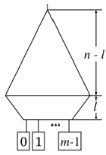
Manage-ment, June 2002. 0 n - l l ... 1 m-1
Figure A.1. Partition of MDD.
[14] L. Xing and Y. Dai, “A new decision-diagram-based method
for efficient analysis on multistate systems,” IEEE
Transac-tions on Dependable and Secure Computing, Vol. 6, No. 3, pp. 161–174, 2009.
[15] S. N. Yanushkevich, D. M. Miller, V. P. Shmerko, and
R. S. Stankovic,Decision Diagram Techniques for Micro- and
Nanoelectronic Design, CRC Press, Taylor & Francis Group, 2006.
[16] X. Zang, D. Wang, H. Sun, and K. S. Trivedi, “A BDD-based algorithm for analysis of multistate systems with multistate
components,” IEEE Transactions on Computers, Vol. 52,
No. 12, pp. 1608–1618, Dec. 2003. APPENDIX
Proof for Theorem 1: Suppose that an MDD is parti-tioned into two parts: the upper and the lower parts as shown in Fig. A.1. In this case, the lower part representsl-variable multi-valued functions, and the upper part represents the function that chooses one from them. The upper part has the maximum number of nodes when it forms a complete valued tree. The number of nodes in the complete multi-valued tree is 1+r+r2+...+rn−l−1. Thus, the maximum
number of nodes in the upper part is
rn−l−1
r−1 . (A.1)
The lower part has the maximum number of nodes when it represents all l-variable multi-valued functions. Since the number of alll-variable multi-valued functions is
mrl, (A.2)
that is the maximum number of nodes in the lower part including terminal nodes. From (A.1) and (A.2), the number of nodes in the MDD is at most
rn−l−1
r−1 +m
rl
.
The number of multi-valued functions which can be rep-resented in the lower part does not exceed the number of functions which can be chosen by the upper part: rn−l.
Therefore, we have the relation:
rn−l≥mrl.