UCC Library and UCC researchers have made this item openly available. Please let us know how this has helped you. Thanks!
Title Constraint programming for optimization under uncertainty in inventory control
Author(s) Rossi, Roberto Publication date 2008
Original citation Rossi, R. 2008. Constraint programming for optimization under uncertainty in inventory control. PhD Thesis, University College Cork. Type of publication Doctoral thesis
Rights © 2008, Roberto Rossi.
http://creativecommons.org/licenses/by-nc-nd/3.0/
Embargo information Not applicable Item downloaded
from http://hdl.handle.net/10468/5871
Constraint Programming for
Optimization Under Uncertainty in
Inventory Control
R
OBERTOR
OSSIA Thesis Submitted to the National University of Ireland
in Fulfillment of the Requirements for the Degree of
Doctor of Philosophy in the Faculty of Science.
October, 2008
Research Supervisors: Dr. S. Armagan Tarim,
Dr. Brahim Hnich, and
Dr. Steven D. Prestwich.
Head of Department: Prof. James Bowen
Department of Computer Science, National University of Ireland, Cork.
Contents
Abstract vi 1 Introduction 1 1.1 Preliminaries . . . 2 1.1.1 Motivations . . . 2 1.1.2 Structure . . . 5 1.2 Formal background . . . 7 1.2.1 Dynamic Programming . . . 7 1.2.2 Constraint Programming . . . 81.2.3 Stochastic Constraint Programming . . . 17
1.2.4 Inventory Control . . . 21
1.3 Related works . . . 34
1.3.1 Stochastic Constraint Programming . . . 34
1.3.2 Stochastic Inventory Control . . . 39
1.3.3 Integration of Operations Research and Constraint Pro-gramming Techniques in Combinatorial Optimization . . . 41
1.4 Thesis Statement . . . 43
1.4.1 Summary . . . 43
1.4.2 Contributions . . . 45
Global chance-constraints . . . 45
Optimization-oriented global chance-constraints . . . 46
A global perspective . . . 46 1.4.3 Paper I (Chap. 2): A Global Chance-Constraint for
1.4.4 Paper II (Chap. 3): Computing Replenishment Cycle
Pol-icy under Non-stationary Stochastic Lead Time [72] . . . 48
1.4.5 Paper III (Chap. 4): Cost-based filtering for stochastic constraint programming [74] . . . 49
1.4.6 Paper IV (Chap. 5): Cost-based Filtering Techniques for Stochastic Inventory Control under Service Level Con-straints [87, 88] . . . 49
1.4.7 Paper V (Chap. 6): Constraint Programming for Stochas-tic Inventory Systems under Shortage Cost [71, 73] . . . . 50
1.5 Future Work . . . 52
1.6 Conclusions . . . 54
2 Paper I: A Global Chance-Constraint for Stochastic Inventory Sys-tems under Service Level Constraints 55 Abstract 55 2.1 Introduction . . . 56
2.2 Formal background . . . 58
2.2.1 Stochastic Programming . . . 59
2.2.2 Constraint Programming . . . 59
2.2.3 Stochastic Constraint Programming . . . 61
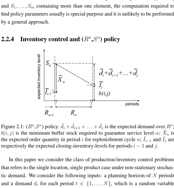
2.2.4 Inventory control and (Rn,Sn) policy . . . . 63
2.3 Existing approaches . . . 64
2.3.1 Stochastic programming model . . . 65
2.3.2 Tarim & Kingsman’s approach . . . 67
2.4 A stochastic constraint programming approach based on global chance-constraints . . . 71
2.4.1 Chance-constraints and policies . . . 71
2.4.2 Global chance-constraints . . . 72
2.4.3 A global chance-constraint for (Rn,Sn) policy . . . . 74
2.4.4 Deterministic equivalent model . . . 75
2.4.5 Propagating the service level global chance-constraint . . 75
2.4.7 Computing the objective function . . . 84
2.4.8 Cost-based filtering . . . 85
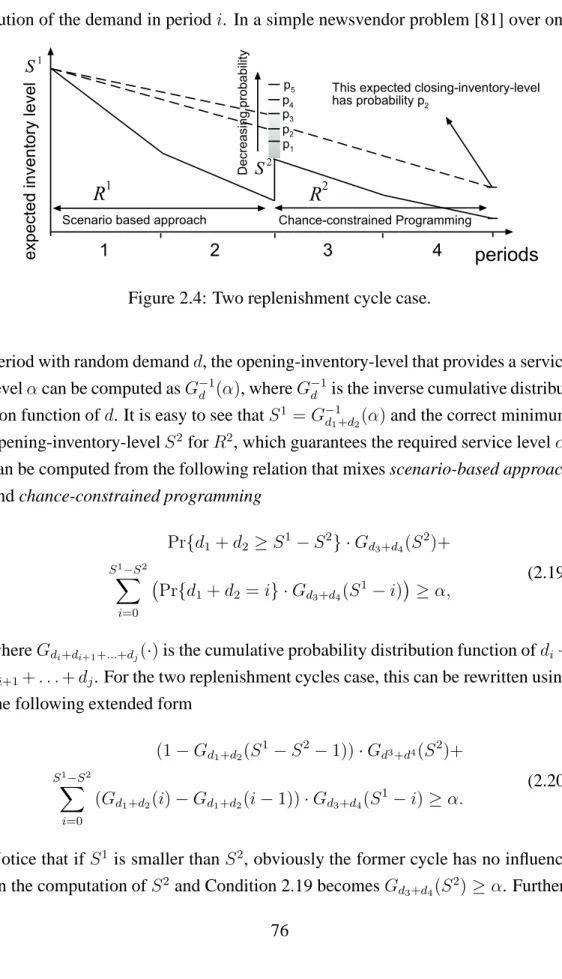
2.5 Comparison with Tarim & Kingsman’s approach . . . 86
2.6 Conclusions . . . 91
3 Paper II: Computing Replenishment Cycle Policy under Non-stationary Stochastic Lead Time 92 Abstract 92 3.1 Introduction . . . 93
3.2 Constraint Programming . . . 95
3.3 Problem Definition . . . 97
3.4 Dynamic Deterministic Lead Time . . . 98
3.5 Non-stationary Stochastic Lead Time . . . 106
3.6 Stochastic Lead Time: a CP Implementation . . . 111
3.7 Experiments . . . 118
3.7.1 Analyzing the cost associated with a set of optimal policy parameters . . . 124
3.8 Conclusions . . . 126
4 Paper III: Cost-based filtering for stochastic constraint programming127 Abstract 127 4.1 Introduction . . . 128
4.2 Formal Background . . . 129
4.3 Value of Stochastic Solutions . . . 130
4.4 Global optimization chance-constraints . . . 132
4.4.1 Expectation-based relaxation for stochastic variables . . . 135
4.4.2 Relaxing the expected value problem . . . 136
4.4.3 Cost-based filtering . . . 137
4.4.4 Finding good feasible solutions . . . 138
4.5 Experimental results . . . 139
4.5.1 Static Stochastic Knapsack Problem . . . 139
4.6 Related works . . . 145
4.7 Conclusions . . . 145
5 Paper IV: Cost-based Filtering Techniques for Stochastic Inventory Control under Service Level Constraints 147 Abstract 147 5.1 Introduction . . . 148
5.2 A CP model . . . 152
5.2.1 Domain pre-processing . . . 156
5.3 From pre-processing to cost-based filtering . . . 157
5.3.1 Tighter upper bounds for optimal replenishment cycle lengths158 5.3.2 Merging adjacent non-replenishment periods . . . 167
5.4 Cost-based filtering by relaxation . . . 175
5.4.1 Tarim’s relaxation . . . 176
5.4.2 Tarim’s relaxation as a shortest path problem . . . 177
5.4.3 Cost-based filtering . . . 178
Partial assignments forδkdecision variables . . . 179
Partial assignments forI˜kdecision variables . . . 180
5.5 Experimental results . . . 180
5.5.1 Effectiveness of filtering methods . . . 181
5.5.2 Comparison with state-of-the-art results . . . 182
5.5.3 More extensive tests . . . 183
5.6 Conclusions . . . 189
5.7 Appendix . . . 190
5.7.1 Considering a unit production costp . . . 190
5.7.2 Proof: Replenishment cycle length bound . . . 191
5.7.3 Modified Dijkstra’s Shortest Path Algorithm . . . 193
6 Paper V: Constraint Programming for Stochastic Inventory Systems under Shortage Cost 196 Abstract 196 6.1 Introduction . . . 197
6.2 Problem definition and(Rn, Sn)policy . . . 199
6.2.1 Stochastic cost component in single-period newsvendor . 202 6.2.2 Stochastic cost component in multiple-period newsvendor 203 6.2.3 Upper-bound for opening inventory levels . . . 206
6.2.4 Lower-bound for expected closing inventory levels . . . . 207
6.3 Deterministic equivalent CP formulation . . . 207
6.4 Comparison of the CP and MIP approaches . . . 212
6.4.1 Cost-based filtering by relaxation . . . 216
6.5 Experimental Results . . . 220
6.6 Conclusions . . . 221
Abstract
Constraint Programming (CP) is a programming paradigm where relations be-tween variables can be stated in the form of constraints. CP features discrete domains and global constraints. Global constraints capture interesting substruc-tures of a problem, encapsulate dedicated inference algorithms based on feasi-bility and/or optimality reasoning, and provide information to the search process on the most viable course. Stochastic Constraint Programming (SCP) is a novel framework that generalizes CP to stochastic problems, allowing both to model and solve this class of problems by using any available existing CP solver. Although this framework proves to be extremely flexible in terms of modeling power, its current implementation does not scale well.
In order to enhance this framework, in this dissertation we propose a gen-eral extension for SCP: global chance-constraints. In contrast to global con-straints, which represent relations among a non-fixed number of decision vari-ables, global chance-constraints represent relations among a non-fixed number of decision variables and stochastic variables. Nevertheless, as global constraints do, global chance-constraints encapsulate dedicated inference algorithms based on feasibility and/or optimality reasoning and may provide information to the search process. We call optimization-oriented global chance-constraints those global chance-constraints performing optimality reasoning.
We applied global chance-constraints encapsulating dedicated inference algo-rithms based on feasibility and/or optimality reasoning to problems in the area of stochastic inventory control. Our computational experience shows that global chance-constraints let us model and solve to optimality problems that could not or could be only approximately solved by other existing approaches. It also shows that filtering based on optimality reasoning is extremely effective for this class of problems.
Roberto Rossi, Cork Constraint Computation Centre, University College Cork, College Road, Cork, Ireland.
Declaration
This dissertation is submitted to University College Cork, in accordance with the requirements for the degree of Doctor of Philosophy in the Faculty of Science.
Parts of this dissertation are the results of collaboration with Dr. Armagan Tarim, Dr. Brahim Hnich and Dr. Steven D. Prestwich. I declare that I have made a substantial contribution to this work and this dissertation is composed by myself. This dissertation has not been submitted to any other university or higher education institution, or for any other academic award in this university. Where use has been made of other people’s work, it has been fully acknowledged and referenced.
The papers contained in this dissertation, or upon which this dissertation is based, have either been published in, been accepted for publication at, or been submitted for publication to, as indicated, at reviewed journals, conferences or workshops.
The papers have not been edited except to fix typographical or spelling errors and to update references. They have, however, been reformatted for this disserta-tion and thus floating objects, such as figures and tables, may have moved about with respect to their surrounding text.
Paper I S. A. Tarim, B. Hnich, R. Rossi, and S. Prestwich, “A Global Chance-Constraint for Stochastic Inventory Systems under Service Level Con-straints”, Constraints, an International Journal, Vol. 13(4):490-517, 2008
Paper II R. Rossi, S. A. Tarim, B. Hnich and S. Prestwich, “Computing Replen-ishment Cycle Policy under Non-stationary Stochastic Lead Time”,
submitted for possible publication to the International Journal of Pro-duction Economics
Paper III R. Rossi, S. A. Tarim, B. Hnich, and S. Prestwich, “Cost-based filter-ing for stochastic constraint programmfilter-ing”, In proceedfilter-ings of The 14th
International Conference on Principle and Practice of Constraint Pro-gramming (CP-2008), Sep. 14-18, 2008 - Sydney, Australia, Lecture
Notes in Computer Science, Springer-Verlag, LNCS 5202, pp.235-250, 2008
Paper IV R. Rossi, S. A. Tarim, B. Hnich, and S. Prestwich, “Cost-based Filter-ing Techniques for Stochastic Inventory Control under Service Level Constraints”, Constraints, an International Journal, forthcoming, 2009. Extended version of: S. A. Tarim, B. Hnich, R. Rossi, and S. Prestwich, “Cost-Based Filtering for Stochastic Inventory Control”, Recent
Ad-vances in Constraints: 11th Annual ERCIM International Workshop on Constraint Solving and Constraint Logic Programming, CSCLP 2006 Caparica, Portugal, June 26-28, 2006 Revised Selected and Invited Papers, Lecture Notes in Computer Science, Springer-Verlag, LNCS
4651, pp.169-183, 2007
Paper V R. Rossi, S. A. Tarim, B. Hnich and S. Prestwich, “Constraint Program-ming for Stochastic Inventory Systems under Shortage Cost”, submit-ted for possible publication to the European Journal of Operational Re-search. Extended version of: R. Rossi, S. A. Tarim, B. Hnich, and S. Prestwich, “Replenishment Planning for Stochastic Inventory Sys-tems with Shortage Cost”, In proceedings of The Fourth International
Conference on Integration of AI and OR Techniques in Constraint Pro-gramming for Combinatorial Optimization Problems (CP-AI-OR 07), May 23-26, 2007, Brussels, Belgium, Lecture Notes in Computer
Some of these papers are reprinted with the permission of the publishers. I will provide more details concerning joint work. In Chapter 2 (Paper I), I proposed the original idea of global chance-constraint, I developed the related software and I have written most of the articles. In Chapter 3 (Paper II), the motivation comes from Dr. Tarim, who first suggested to consider a stochastic lead time in our model. We developed together the mathematical model and I implemented the related software on my own. Again I have written most of the articles with the invaluable support of Dr. Hnich. The motivation for Chapter 4 (Paper III) comes from Dr. Tarim and myself. In particular the use of Jensen’s inequality was firstly suggested by Dr. Tarim. Nevertheless I proposed the idea of
optimization-oriented global chance-constraint in which this inequality is used to
generate bounds and perform filtering. I also identified the motivation problems and I implemented the software for running the experiments. Chapter 5 (Paper IV) presents ideas proposed by Dr. Tarim, Dr. Hnich and myself. Specifically I proposed the filtering strategy presented in Section 5.3.1. I implemented all the related software and also a graphical interface for visualizing results. I wrote most of the article. Finally, Chapter 6 (Paper V) presents ideas that I originally proposed, implemented, and put together in a conference paper first, and then in a journal article. Also in this case Dr. Tarim, Dr. Hnich and Dr. Prestwich made important comments and had an active role in the writing of the research articles.
Roberto Rossi July 2008.
Dedication
To my family.Acknowledgements
Roberto Rossi is supported by Science Foundation Ireland (SFI) under Grant No. 03/CE3/I405 as part of the Centre for Telecommunications Value-Chain Research (CTVR) and Grant No. 05/IN/I886.
After the formal acknowledgements, I would like to thank in this small part of my dissertation all the people that contributed to my personal and professional development during my PhD.
I will list people in chronological order to be fair with everyone. I want to thank Michela Milano, who sent me to Cork three years ago and made me dis-cover this incredible community of researchers. I am very grateful to the people in Cork who hosted me for my first six months and believed in me letting me stay for the following three years: Armagan Tarim and Brahin Hnich. I will never for-get our first lunch at Mercury Lounge (now closed down) and Gusto (still doing great business with 4C) and I will never forget our brainstorming sessions at 4C. I want to thank my (official) supervisor Steve Prestwich, who has been extremely supportive during my all PhD and in the last 2 years in particular, when both Ar-magan and Brahim left for the sunny Turkey. I want also to thank all the people of the Cork Constraint Computation Centre (4C) with who I had fruitful discussions and great laughters during pool tournaments, barbecues and other nice events. 4C has been an incredibly stimulating place for research. A special thank goes to Eleanor, Linda and Caitriona for all the administrative support. I wish to thank the people in Bell Labs Ireland for hosting me several times in Dublin and for the time of work and leisure we had. I am grateful to my family that did everything was possible to make me study and to let me get where I am now. Finally I am grateful to Lauren, for sharing with me in the last two years all the good and bad things of our life.
Chapter 1
Introduction
1.1
Preliminaries
In this section we firstly provide the motivations for the work presented in this dissertation; secondly we briefly state the topic discussed in this dissertation; and finally we discuss the structure of the rest of this chapter.
1.1.1
Motivations
Many computational problems can be described in terms of restrictions imposed on the set of possible solutions, and Constraint Programming is a problem-solving technique that works by incorporating those restrictions in a programming envi-ronment. It draws on methods from combinatorial optimization and Artificial In-telligence, and has been successfully applied in a number of fields from schedul-ing, computational biology, finance, electrical engineering and Operations Re-search through to numerical analysis.
Constraint Programming has been extremely successful in the field of deter-ministic production planning and scheduling [47]. The commercial success of off-the-shelf tools such as ILOG Scheduler [49] is remarkable.
Nevertheless, real-life management decisions are usually made in uncertain environments. Random behavior such as the weather, lack of essential exact in-formation such as the future demand, incorrect data due to errors in measurement, and vague or incomplete definitions, exemplifies the theme of uncertainty in such environments.
In this work we aim to investigate the application of Constraint Programming to decision problems under uncertainty and in particular to production/inventory control problems. Having an effective means to handle these problems is a key to profitability for retail business, which is particularly affected by uncertainty. Supply chains are plagued by uncertainty associated with customers’ demand, lead-times, suppliers’ capacity, and so forth. We now provide some evidence of the impact that uncertainty has on retail and on the importance of having state-of-the-art decision support systems for hedging against it.
Retail replenishment†is a high-value activity. According to the US Commerce
Department, $1.1 trillion in inventory supports $3.2 trillion in annual US retail sales. This inventory is spread out across the value chain, with $400 billion at retail locations,$290 billion at wholesalers or distributors and$450 billion with manufacturers. This is a colossal amount of capital tied up in inventory [...]. Improving distribution centre efficiency of just a few percentage points through advanced automation and real-time replenishment may deliver significant savings and require less capital to be tied up in inventory.‡
Table 1.1 shows inventory as a percentage of total assets for some major in-dustries. It appears that such an amount of inventory should significantly reduce
Industry Inventory relative to total assets
Automotive dealers and service stations (retail) 53.81% Apparel and accessory stores 41.14% Building materials, garden supplies and mobile home dealers (retail) 40.09%
Food stores 33.52%
Electrical and electronic equipment 19.57%
Total construction 17.20%
Table 1.1: Inventory as a percentage of total assets for some major industries. Data source: Internal Revenue Service, U.S. Treasury Department, Statistics of Income, 1977; Corporate Income Tax Returns (Washington, DC: Government Printing Of-fice, 1982), pp. 27-34.
the probability of stock-out§at retail level. In fact, many surveys reveal that what happens in reality is that a high percentage of shoppers, on average, fail to find products in stock. Stock-out events for many firms represent a significant portion of all retail sales. Even if some of these events are actually recouped via alterna-tive products, still the lost sales faced by these firms remain high. Obviously this is seriously affecting both retail margins and customer satisfaction. Overstocks¶, on the other hand, can be just as damaging financially to the organization. Nowa-days no retailer can afford to tie up capital unnecessarily in inventory, or risk lost sales and dissatisfied customers due to stock-outs. However, current practices put picking location, or to another mode of storage in which picking is performed.
‡“The Future of Retail Replenishment”, Manhattan Associates c, 2006,
http://www.manh.com/library/MANH-TechVis Whitepaper.pdf
§When at a given moment in a given inventory there is not the quantity of a part or a product
that is demanded. A stock-out occurs in a distribution center when there are orders that can not be filled within their due date.
in place by firms seem unable to produce a balanced situation where the right good is in the right place at the right time. High stockout levels in retail settings prove to be the norm, rather than the exception. As a study conducted in 1996 by the Andersen Consulting Group — today known as Accenture — revealed, on a typical afternoon in a typical US supermarket, 8.2% of items are out of stock, and this number is nearly doubled for items that are advertised. In 3.4% of stock-outs, consumers refuse to buy an alternative and often take their business to the competition. The costs of stockouts in US supermarkets alone are estimated at $7-12 billion of sales. This example illustrates the drastic consequences of stock-outs, and underlines the importance of properly managing inventory investments by means of sound modeling techniques and advanced decision support systems.
In the last few decades the Operations Research community developed a large amount of lore for decision making under uncertainty. Stochastic Programming (see Sengupta [78], Vajda [95], Kall and Wallace [54]) has been widely and suc-cessfully applied to problems from the retail world.
In contrast to what has happened in the Operations Research community with Stochastic Programming, only recently the Constraint Programming community has started to formalize general approaches that employ Constraint Programming for optimization under uncertainty. The probabilistic CSP framework [29] has been one of the first work in this direction. Relevant works are also Partial CSPs [36] and Soft CSPs [13]. Nevertheless, none of these approaches is as general as the techniques employed in Stochastic Programming. The very first step to-wards the integration of Constraint Programming and Stochastic Programming was made by Walsh, who introduced Stochastic Constraint Programming [98] a novel framework able to fully represent the stochastic nature of decision problems under uncertainty. Stochastic Constraint Programming is still a young field, and only recently a general purpose modeling and solution framework was proposed for stochastic constraint programs in [91]. There are still several issues open both in terms of expressiveness of the framework and of efficiency of the current solu-tion methods available. Applicasolu-tions to real world problems are also very limited. In this sense Stochastic Constraint Programming is indeed an interesting “green field” for research.
ben-efits in the field of stochastic inventory/production control. The results we present in this work fully support this thesis. In fact we propose Stochastic Constraint Programming approaches for inventory control that are:
• more accurate than other existing approaches in the literature. The quality
of the solution found is improved significantly, i.e. costs are reduced, and the expected cost predicted is closer to that realized in practice;
• more effective in terms of computational performance. Our Constraint
Pro-gramming reformulations proved to be orders-of-magnitude more efficient than other approaches in the literature;
• more effective in terms of expressiveness. Constraint programming
refor-mulations are particularly compact and, as shown in [92], require fewer constraints and decision variables than other existing approaches in the lit-erature.
As discussed above, large amount of capital are invested in inventories by firms. Having more effective, accurate and efficient approaches to inventory optimiza-tion is therefore desirable. The research presented in this dissertaoptimiza-tion tries to pursue these objectives.
Topic. In this dissertation we investigate the application of Stochastic Con-straint Programming techniques and in particular of global chance-conCon-straints, a novel modeling concept introduced here, in the area of stochastic inventory con-trol. We implemented global chance-constraints encapsulating dedicated infer-ence algorithms based on feasibility and/or optimality reasoning. Our computa-tional experience shows that global chance-constraints let us model and solve to optimality problems that could not or could be only approximately solved by other existing approaches. It also shows that filtering based on optimality reasoning is extremely effective for this class of problems..
1.1.2
Structure
• in Section 1.2, we provide the relevant formal background in Dynamic Pro-gramming, Constraint ProPro-gramming, Stochastic Constraint ProPro-gramming, and inventory control;
• in Section 1.3, we discuss the relevant literature in Stochastic Constraint Programming and stochastic inventory control; then we also discuss exist-ing techniques for integratexist-ing Operations Research and Constraint Program-ming approaches in Combinatorial Optimization;
• in Section 1.4, we summarize the content of this dissertation, we state at a high level our contributions, and finally for each of the following chapters we list the respective contributions in details;
• in Section 1.5, we discuss possible future research directions. Specifically, for each of the following chapters we discuss which questions remain open and which directions may be interesting to follow in the future research;
• in Section 1.6, we draw conclusions.
The general structure of this dissertation will be further discussed in Section 1.4.
1.2
Formal background
In this section we discuss the relevant formal background in the areas of Dy-namic Programming (Section 1.2.1), Constraint Programming (Section 1.2.2) and Stochastic Constraint Programming (Section 1.2.3), a framework that employs Constraint Programming for solving decision problems under uncertainty. Finally we discuss relevant topics in stochastic inventory control (Section 1.2.4).
1.2.1
Dynamic Programming
This section is mainly based on [33].
Dynamic Programming (DP) is an optimization procedure that solves opti-mization problems by decomposing them into a nested family of subproblems. The core of DP is the principle of optimality [8, 25].
In DP a problemP is associated with a state space graphSG= (S, T)where each element of the vertex set S is a state and each element of the arc set T
represents a feasible transition between two states. The original problem is solved by solving a shortest path problem in the state space graph from an initial state to a final state (boundary condition)k. If the original problem is NP-hard, the corresponding state space graph will have an exponential number of nodes.
Consider a discrete system defined onnsteps. Each step is characterized by:
• a final state sk that represents the system at the end of step k. sk ∈ Sk,
whereSkis the set of feasible states at the end of stepk.
• a decision variablexkthat represents a decision taken at step k. xk ∈ Xk,
whereXkis the set of feasible decisions that could be taken at stepk.
• a cost/profit function pk(sk, xk) representing the cost/profit achievable in
stepk ifskis the final state andxk the decision considered.
• a state transition tk(sk−1, xk) that leads the system toward the statesk =
tk(sk−1, xk).
Without loss of generality we will here refer to minimization problems. Op-timization problems aim at finding the set of optimal values to be assigned to decision variables such that the following objective function is minimized:
z = min ( n X k=1 pk(sk, xk) ) .
To determine the value of z, DP solves a set of problems i = 1, . . . , n, each corresponding to a system composed by isteps and characterized by the statesi
at the end of stepi. The recursive formulation of the cost function at stepiis:
fi(si) = min xi∈Xi min si∈Si−1{ fi−1(si−1) +pi(si, xi)}
wheresi =ti(si−1, xi). In addition, we have the following boundary condition:
f1(s1) = min
x1∈X1{
p1(s1, x1)}
wheres1 =t1(s0, x1).
DP is based on the principle of optimality [8] stating that an optimal policy is such that given whatever state si, and the decision xi, the decisionsx1, . . . , xi−1
corresponding to the remaining steps constitute an optimal policy w.r.t. the state
si−1resulting from the decision taken at stepi.
DP is often applied to problems requiring a sequence of interrelated decisions, and has been applied to solve a wide variety of combinatorial optimization prob-lems, as well as optimal control problems. Recently, effective hybrid optimization techniques involving DP and Constraint Programming have been proposed in [33]. In Chapters 5 and 6, we develop similar hybrid techniques in order to efficiently solve combinatorial optimization problems for inventory control. In the next sec-tion we formally introduce Constraint Programming.
1.2.2
Constraint Programming
This section is mainly based on [1].
v. In what follows we will restrict our attention to finite domains. Consider a finite set of variablesV ={v1, v2, . . . , vk}, wherek >0, with respective domainsD=
{D1, D2, . . . , Dk}. A constraintC on V is defined as a subset of the Cartesian
product of the domains of the variables inV, i.e. C ⊆D1×D2 ×. . .×Dk. The
cardinality of V, |V|, is the arity of C. C is a unary constraint if it has arity 1, it is a binary constraint if it has arity 2, and it is a non-binary constraint if it has arity k, with k > 2. Finally,C is a global constraint if it is a relation among a non-fixed number of variables.
A Constraint Satisfaction Problem (CSP) [1, 17, 62] is a triplehV,C,Di, where
V = {v1, v2, . . . , vk} is a finite set of variables with respective domains D =
{D1, D2, . . . , Dk}, andC is a finite set of constraints, each of which is defined on
a subset of the variables inV.
Consider a CSPhV,C,Di, a tuple(d1, . . . , dk)∈D1×D2×. . .×Dksatisfies
a constraintCi ∈ Con the variablesvi1, vi2, . . . , vimif(di1, di2, . . . , dim)∈Ci. A
tuple(d1, . . . , dk)∈D1×D2×. . .×Dkis a solution to a CSP if it satisfies every
constraintC ∈ C.
Consider the CSPs P = hV,C,Di andP0 =hV,C0,D0i. P andP0 are called
equivalent if they have the same solution set. P is said to be smaller thatP0 if
they are equivalent andDi ⊆Di0for alli. This relation is written asP P0. P is
strictly smaller thatP0, ifP P0 andD
i ⊂D0i for at least onei. This is written
P ≺P0. When bothP P0andP0 P we writeP ≡P0
Often we want to find a solution to a CSP that is optimal with respect to certain criteria. Consider a CSPhV,C,Di, whereD ={D1, D2, . . . , Dk}. Let S be the
solution set, that is the set of all the tuples(d1, . . . , dk) ∈ D1 ×D2 ×. . .×Dk
that are solutions to the CSP. A Constraint Optimization Problem, or a COP, is a CSP on the solution set of which an objective function,f : S → R, has to be optimized. An optimal solution to a COP is a solution to the CSP that is optimal with respect tof. The objective function value is often represented by a variable
z, together with the “constraint”maximizez orminimizez, respectively for a maximization or a minimization problem.
In Constraint Programming (CP), the goal is to find a solution (or all solutions) to a given CSP, or an optimal solution (or all optimal solutions) to a given COP. A filtering algorithm is typically associated with every constraint. This algorithm
re-moves values from the domains of the variables participating in the constraint that cannot belong to any solution of the CSP. These filtering algorithms are repeat-edly called until no new deduction can be made. This process is called constraint
propagation or propagation in short. In conjunction with this process CP uses
a search procedure (like a backtracking algorithm) where filtering algorithms are systematically applied when the domain of a variable is modified. The solution process interleaves propagation and search to reach the given goal.
Example 1.2.1. Letx1, x2be variables with respective domainsD1 ={0,1,2,3},
D2 = {0,1,2,3,4,5}. Letx3 be a binary variable with domainD3 ={0,1}. On
these variables we impose the following constraints: x1 ≥ 3 x1 +x2 ≥ 8 and
(x2 >0)↔(x3 = 1). We denote the resulting CSP as
x1 ∈ {0,1,2,3}, x2 ∈ {0,1,2,3,4,5}, x3∈ {0,1},
x1 ≥3,
x1+x2 = 8,
(x2 >0)↔(x3 = 1).
A solution to this CSP isx1 = 3,x2 = 5andx3 = 1.
Propagation. Constraint propagation is a process that removes a subset or all the inconsistent values from the domains, by reasoning on the individual con-straints. This process may significantly reduce the search space. Thus constraint propagation is a key instrument to improve the efficiency of CP solvers.
Let C be a constraint on the variables x1, . . . , xm with respective domains
D1, . . . , Dm. A propagation algorithm for C removes values from D1, . . . , Dm
that do not participate in a solution toC. A propagation algorithm does not have to remove all such values, as this may lead to an exponential running time due to the nature of some constraints.
We consider the CSPP =hV,C,Di. P can be transformed into a smaller CSP
P0 by repeatedly applying the propagation algorithm for all constraints inC until
there is no more domain reduction. This process is called constraint propagation. When no more domain reduction can be achieved by iterating the process, we say
that each constraint, and the CSP, is locally consistent and that we have achieved a notion of local consistency on the constraints and the CSP. The term “local consistency” reflects the fact that the CSP obtained through the discussed process is not globally consistent. It is instead a CSP in which all the constraints are “locally”, i.e. individually, consistent. A comprehensive discussion on the process of constraint propagation is given by Apt [1].
If we demand that every domain value of every variable in the constraint be-longs to a solution to the constraint then what we achieve is hyper-arc consistency, that is the strongest local consistency notion for a constraint. This still does not guarantee a solution to the whole CSP because other constraints in it are not con-sidered in such a process.
Example 1.2.2. Consider again the CSP of Example 1.2.1, i.e. variablesx1, x2, x3
with respective domainsD1 = {0,1,2,3}, D2 = {0,1,2,3,4,5}, D3 = {0,1},
and
x1 ≥3, (1.1)
x1+x2 = 8, (1.2)
(x2 >0)↔(x3 = 1). (1.3)
We apply constraint propagation until the constraints are hyper-arc consistent:
x1∈ {0,1,2,3} x2∈ {0,1,2,3,4,5} x3∈ {0,1} (1.1) −→ x1∈ {3} x2∈ {0,1,2,3,4,5} x3∈ {0,1} (1.2) −→ x1∈ {3} x2∈ {5} x3∈ {0,1} (1.3) −→ x1∈ {3} x2∈ {5} x3∈ {1}
The three constraints are examined sequentially, as indicated above the arcs. We first examine constraint 1.1, and deduce that values 0,1 and 2 in D1 do not
appear in a solution to it. Then we examine constraint 1.2, and remove all the values except 5 from D2. This is because 5 is the only value that supports the
remaining value 3 inD1. Finally we examine constraint 1.3 and we remove value
0 fromD3. The resulting CSP is hyper-arc consistent. In fact, we found a solution
to the CSP.
as possible, in fact constraint propagation is applied each and every time a deci-sion variable domain has been changed. This happens very frequently during the solution process. Note that both the efficiency of the propagation algorithms and the order in which the propagation algorithms are applied directly influences the efficiency of constraint propagation.
Search. In the solution process CP employs a search tree. A search tree is com-posed by a set of vertices, or nodes, and a set of arcs, or branches. A nodev is a
direct descendant of a nodeuand, conversely,uis the parent ofv, if (u, v) is an arc of a search tree.
Definition 1.2.1 (Search tree [1]). LetP be a CSP with a sequence of variables
X. A search tree forP is a (finite) tree such that
• its nodes are CSPs,
• its root isP,
• ifP1, . . . , Pmwherem >0are all direct descendants ofP0, then the union
ofP1, . . . , Pmis equivalent w.r.t.X toP0, for every nodeP0.
A nodeP of a search tree is at depthdif the length of the path from the root toP isd.
In CP, a search tree is dynamically built by splitting a CSP into smaller CSPs, until we reach an inconsistency , i.e. some decision variable domain becomes empty, or a solution to the CSP. There are two possible ways to split a CSP into smaller CSPs: we can either split a constraint (for instance a disjunction) or split the domain of a variable. The second being the most common technique.
A direct consequence of what we discussed is that a CSP is associated with each node in the search tree. At each node we can therefore apply constraint propagation and we may detect that the corresponding CSP is inconsistent, or we may achieve some domain reduction for it. Obviously, in both cases we will generate and explore less nodes, this is the reason why constraint propagation can speed up the solution process. However, in order to do so, constraint propagation must be efficient. This means that the time spent on propagation should be less than the time that is gained by it.
In splitting the domain of a variable, we first select a variable and then decide how to split its domain. This process is guided by variable and value ordering
heuristics. These heuristics impose an ordering on the variables and values,
re-spectively. The ordering imposed by these heuristics has a great impact on the search process.
First we give the following definitions that are relevant to introduce variable and value ordering heuristics. A relationon a setSis called a partial order if it is reflexive (s sfor alls ∈ S), transitive (s tandt uimpliess u), and antisymmetric (s tandt simpliess= t). A partial orderis a total order ifs t ort sfor allt, s ∈ S. Given a partial orderon a set s, an element
s ∈ S is called a least element ifs t for allt ∈ S. Two elementss, t∈ S are
incomparable with respect toifstandt s.
A variable ordering heuristic imposes a partial order on the variables with non-singleton domains. The most constrained first variable ordering heuristic is of common use. Variables are ordered according to the respective number of oc-currences in the constraints. A variable that appears the most often, is ordered least. The ratio behind this is that, most likely, changing the domains of such vari-ables will cause more values to be removed by constraint propagation. Another variable ordering heuristic is the smallest domain first heuristic, also known as the first fail heuristic. Variables are ordered, in this heuristic, with respect to the size of their domains. A variable that has the smallest domain is ordered least. By using this heuristic less nodes are generated in the search tree and inconsistent CSPs are detected earlier. If two or more variables are incomparable, a common strategy is to apply the lexicographic ordering to the variables in order to obtain a total order.
A value ordering heuristic induces a partial order on the domain of a variables. Values in the domains are ordered according to a certain criterion, such that val-ues that are ordered least are selected first. For instance, the lexicographic value ordering heuristic orders the values according to a lexicographic ordering. The
random value ordering heuristic, instead, orders the variables randomly.
Simi-larly to what discussed for the variable ordering heuristics, if a value ordering heuristic imposes a partial order on a domain, we can apply the lexicographic or random value ordering heuristic to incomparable values in order to create a total
order. A value ordering heuristic is also referred to as branching heuristic because it decides the order of the branches in the search tree.
A domain splitting procedure is applied after a variable has been selected and a value ordering heuristics imposed a total order on its domain. Given a domain, a domain splitting procedure generates a partition of the domain. Con-sider a domain D = {d1, d2, . . . , dm} and a total order such thatd1 d2
. . . dm. Two common domain splitting procedures are labeling and
bisec-tion. Labeling splits Dinto {d1},{d2}, . . . ,{dm}. In practice the labeling
pro-cedure is often implemented to split a domain D into {d1},{d2, . . . , dm}. This
procedure is also called enumeration in the literature. Bisection splits D into
{d1, . . . , dk},{dk+1, . . . , dm}, wherek=bm/2c.
Consider a CSPP0 =hV,C,Diand a variablev ∈ V whose domain has been
split into the partition D1, . . . , Dk. Then we define the direct descendants ofP0
as Pi = hV,C ∪ {v ∈ Di},Di for i = 1, . . . , k. In practice, we modify the
domain of a variable instead of adding a constraint to define a descendant. If the partition “respects” the value ordering heuristic that was applied to the domain, i.e.di djfor alldi ∈Di,dj ∈Dj,i < jandi= 1, . . . , k−1, the corresponding
descendants inherit the ordering of the value ordering heuristic, i.e. P1 . . .
Pk.
A search strategy defines the traversal of the search tree. Assume that all the direct descendants of a node in a search tree are totally ordered, for instance according to the given value ordering heuristic. The least element corresponds to the first descendant.
Depth-first search (DFS): starting from the root node, proceed by descending to its first descendant. Continue until a leaf is reached, then backtrack to the parent of the leaf and descend to its next descendant, if it exists. Continue the process until the root node is reached again and all its descendants have been visited. DFS is a complete (or exact) search strategy, not redundant. This means
that it explores all paths from the root to a leaf exactly once. In DFS backtracking to a previous node only takes place after we have visited a leaf. This leads to the more general notion of depth-first based search strategies.
Depth-first based search strategies: we start at the root node and we pro-ceed by descending to its first descendant. This process continues until a leaf
is reached. Then we backtrack to some previously visited node and descend to its next descendant, if it exists and if it is allowed. This process continues until all leafs have been visited. Other examples of depth-first based search strategies,
in addition to DFS, are limited discrepancy search or LDF [38], depth-bounded discrepancy search or DDS [97], and discrepancy-bounded depth-first search, or DBDFS [7].
Optimization. By recalling that a COP consists of a CSP together with an ob-jective functionf, it is easy to see why the search for an optimal solution (or all the optimal solutions) to a COP operates in a similar fashion to the search for a solution to a CSP. By restricting (without loss of generality) ourselves to mini-mization problems, we represent the objective value using a variable z. When a solutions to the CSP is found, the corresponding value ofz, sayz =β, represents an upper bound for the optimal value of f. It follows that we can add the con-straintz < βto all the CSPs in the search tree and continue. This will, in practice, replace the maximum value in the domain ofz withβ.
Example 1.2.3. We present the solution process of CP, using the following COP
P0: x1 ∈ {3,8}, x2 ∈ {0,1,2,3,4,5}, x3∈ {0,1}, minimizez, z =x1+ 6x3, x1 ≥3, x1+x2 = 8, (x2 >0)↔(x3 = 1).
To build a search tree, we apply the lexicographic variable and value ordering heuristic and use labeling as domain splitting procedure. As search strategy we use DFS. At each node we apply hyper-arc consistency constraint propagation. The CSP P0 is the root. The search tree is depicted in Fig. 1.1. We first apply
P
1P
2P
0x
1Î
{3}
x
1Î
{8}
Figure 1.1: The search tree of Example 1.2.3
constraint propagation toP0. It follows that
x1 ∈ {3,8}, x2 ∈ {0,5}, x3 ∈ {0,1}, z∈ {8,9}.
We select the lexicographically least variable, x1, split its domains into{3}and {8}, and generate the descendants P1 and P2 where P1 = P0 ∪ x1 ∈ {3} and
P2 =P0 ∪x1 ∈ {8}.
We descend to nodeP1and apply constraint propagation. It follows that
x1 ∈ {3}, x2∈ {5}, x3 ∈ {1}, z ∈ {9}.
We have found a solution with z = 9. Hence we add to all CSPs the constraint
z <9.
Next we backtrack to P0, descend toP2, and apply constraint propagation. It
follows that
x1 ∈ {8}, x2∈ {0}, x3 ∈ {0}, z ∈ {8}.
We have found a solution with z = 8. Hence we add to all CSPs the constraint
z < 8. Next we backtrack toP0 and stop because all its descendants have been
visited.
We return the optimal solution we found in leafP2.
Optimization-oriented global constraints embed an optimization compo-nent, representing a proper relaxation of the constraint itself, into a global con-straint [32]. The relaxation employed can be a continuous relaxation, as in the examples provided in [32], a DP relaxation, as discussed in [33], or it can be
any other suitable relaxation. The optimization component provides three pieces of information: (a) the optimal solution of the relaxed problem; (b) the optimal value of this solution representing an upper bound on the original problem objec-tive function; (c) a gradient function grad(V,v), which returns for each couple
variable-value (V,v) an optimistic evaluation of the profit obtained ifvis assigned to V. These pieces of information are exploited both for propagation purposes and for guiding the search.
1.2.3
Stochastic Constraint Programming
In order to extend CP to decision problems under uncertainty, Walsh [98] proposed an extension of CP called Stochastic Constraint Programming (SCP) in which there is a distinction between decision variables, which can be set freely, and stochastic (or observed) variables, which follow some probability distribution.
We first provide some basic notions on probability theory.
Probability theory. In probability theory uncertainty is represented in terms of random experiments. Let ω be an outcome of an experiment, the set of all the possible outcomes is represented byΩ.
Subsets of Ω are called events, which combine one or more outcomes. We denote byAa collection of random events.
To each eventA ∈ Ais associated a value Pr{A}, called a probability, such that0 ≤ Pr{A} ≤ 1, Pr{∅} = 0, P r{Ω} = 1 andPr{A1 ∪A2} = Pr{A1}+
Pr{A2}ifA1∩A2 =∅.
The triplethΩ,A,Priis called a probability space that must satisfy a number of conditions (see, e.g, [54]). Several random variables associated with a prob-ability space can be defined, namely, all the variables that are influenced by the random events inA.
In some cases the elements ω ∈ Ω are used to describe a few states of the
world or scenarios. All random elements then jointly depend on these finitely
many scenarios.
For a particular random variable ξ, its cumulative distribution is defined as
A discrete random variable takes a finite or countable number of different values. It is described by its probability mass function. This is the list of possible valuesξk,k ∈K, with associated probability
fξ(ξk) = Pr{ξ=ξk},
such thatPk∈Kfξ(ξk) = 1.
Continuous random variables can often be described through a so-called
den-sity function fξ(ξ). The probability of ξ being in an interval [a, b] is obtained
as Pr{a≤ξ≤b}= Z b a fξ(ξ)dξ, or equivalently Pr{a≤ξ≤b} = Z b a dFξ(ξ),
whereFξ(.)is the cumulative distribution as earlier. Contrary to the discrete case,
the probability of a single valuePr{ξ=a}is always zero for a continuous random variable. The distributionFξ(.)must be such that
R∞
−∞dFξ(ξ) = 1.
The expectation of a random variable is computed asµ = Pk∈Kξkfξ(ξk)or
µ=R−∞∞ ξdFξ(ξ)in the discrete and in the continuous case, respectively.
The variance of a random variable isE[(ξ−µ)2], whereE[.]denotes the
ex-pectation.
The expectation of ξr is called ther-th moment of ξ. A point ηis called the
α-quantile ofξif and only if for0< α <1,η= min{x|Fξ(x)≥α}.
Letφ :R→Rbe a convex function andξa random variable. Thenφ(E[ξ])≤
E[φ(ξ)](Jensen’s inequality).
Equipped with these notions, we now formally introduce SCP.
Semantics. A stochastic CSP is defined as a 6-tuplehV, S, D, P, C, θi, whereV
is a set of decision variables andSis a set of stochastic variables,Dis a function mapping each element ofV and each element ofSto a domain of potential values. A decision variable in V is assigned a value from its domain. P is a function mapping each element ofSto a probability distribution for its associated domain.
inSis a chance-constraint. θhis a threshold value in the interval[0,1], indicating
the minimum satisfaction probability for chance-constrainth. Note that a chance-constraint with a threshold of 1 (or without any explicit threshold specified) is equivalent to a hard constraint.
A stochastic CSP consists of a number of decision stages. A decision stage is a pairhVi, Sii, whereVi is a set of decision variables and Siis a set of stochastic
variables.
One-stage Stochastic CSP. In a one-stage stochastic CSP, a single stage is con-sidered,hV, Si, and the decision variables are set before observing the realizations of the stochastic variables. A solution can be therefore expressed as an assignment for decision variables inV such that, given random values for stochastic variables inS, the hard constraints are satisfied and the chance-constraints are satisfied in the specified fraction of all possible scenarios.
m-stage Stochastic CSP. In anm-stage stochastic CSP,V andSare partitioned into disjoint sets, V1, . . . , Vm and S1, . . . , Sm, and we consider multiple stages,
hV1, S1i,hV2, S2i, . . . ,hVm, Smi. A decision variablexi ∈Vjis set to a value only
after realizations of stochastic variables
n yi yi ∈Sjt=1−1St o
in former stages have been observed. To solve anm-stage stochastic CSP an assignment to the variables in V1 must be found such that, given random values forS1, assignments can be
found forV2such that, given random values forS2, ..., assignments can be found
for Vm so that, given random values for Sm, the hard constraints are satisfied
and the chance constraints are satisfied in the specified fraction of all possible scenarios. The solution of anm-stage stochastic CSP is represented by means of a policy tree [91]. A policy tree is a set of decisions where each path represents a different possible scenario and the values assigned to decision variables in this scenarios.
Stochastic Constraint Optimization. Let S denote the space of policy trees representing all the solutions of a stochastic CSP. We may be interested in finding a feasible solution, i.e. a policy tree s ∈ S, that maximizes the value of a given objective function f(·)over the stochastic variables S (edges of the policy tree)
and over a subsetVb ⊆ V of the decision variables (nodes in the policy tree). A
Stochastic COP is then defined in general as
max
s∈S f(s).
Solution methods. Two solution methods have been proposed so far in the liter-ature: the first relies on backtracking and forward checking algorithms proposed in [98], the second [91] adopts a scenario based approach.
Policy based view. In the policy based view of [98], the semantics is based on a tree of decisions. Each path in a policy represents a different possible scenario (set of values for the stochastic variables), and the values assigned to decision variables in this scenario. To find satisfying policies, backtracking and forward checking algorithms, which explores the implicit AND/OR graph, are presented. Stochastic variables give AND nodes as we must find a policy that satisfies all their values, whilst decision variables give OR nodes as we only need find one satisfying value. In [5] the authors extend the forward checking procedure to better take advantage of probabilities and thus achieve stronger pruning. They also define arc consistency for stochastic CSPs and introduce an arc consistency algorithm that can handle constraints of any arity.
Scenario based approach. In a scenario based approach [11, 91], a scenario tree is generated which incorporates all possible realization of discrete random variables into the model explicitly. A path from the root to an extremity of the event tree represents a scenarioω∈Ω, whereΩis the set of all possible scenarios. With each scenario a given probability is associated. IfSi is theith random
vari-able on a path from the root to the leaf representing scenarioωandai is the value
given toSi in theith stage of this scenario, then the probability of this scenario
is given byPr{ω} = QiPr(Si = ai). Within each scenario, we have a
conven-tional (non-stochastic) constraint program to solve. All we have to do is replacing the stochastic variables by the values taken in the scenario and ensure that the values found for the decision variables are consistent across scenarios as certain decision variables are shared across scenarios. Constraints are defined (as in
tradi-tional constraint satisfaction) by relations of allowed tuples of values, and can be implemented with specialized and efficient algorithms for consistency checking. The great advantage of this approach is that conventional constraint solvers can be used to solve stochastic constraint programs. The scenario-based view of stochas-tic constraint programs also allows later stage stochasstochas-tic variables to take values which are conditioned by the earlier stage stochastic variables. This is a direct consequence of employing the scenario representation, in which stochastic vari-ables are replaced with their scenario dependent values. Of course, there is a price to pay as the number of scenarios grows exponentially with the number of stages. For this reason, the authors also proposed several approximate solution methods based on scenario reduction methods. We here mention two of the reduction ap-proaches employed. The “most likely scenario” approach only consider a few of the most probable scenarios and ignore rare events. Latin Hypercube Sampling [84] ensures that the ensemble of random numbers is representative of the real variability whereas traditional random sampling (sometimes called brute force) is just an ensemble of random numbers without any guarantee.
1.2.4
Inventory Control
In the previous sections we formally introduced CP and its extension for decision problems under uncertainty, SCP. We now introduce the relevant formal back-ground in inventory control, since the rest of this dissertation will extensively discuss the application of SCP techniques to inventory control problems.
This section is mainly based on [81].
Lot-sizing is a very active research area in combinatorial optimization.
Ana-lyzing and controlling inventory systems that have to cope with dynamic demand patterns is a challenging task [14, 30]. Therefore it does not surprise that control-ling stochastic inventory systems is even harder and that stochastic multi-period lot-sizing problems currently represent a challenging research area [100]. In the following sections we will provide some background on stochastic lot-sizing.
In lot-sizing problems, when the demand is assumed to be stochastic, the cost of insufficient capacity in the short run — that is the cost associated with shortages, or with averting them — assumes a great importance. The problem in
stochastic lot-sizing is typically to determine the “correct” quantity of buffer (or safety) stocks that must be kept to meet unexpected fluctuations of the demand. There are several possible choices for the shortage costing method or for the cus-tomer service level measure. In what follows we will firstly recall the Newsvendor problem, probably the most studied problem in stochastic lot-sizing, and then we will extend the discussion to multi-period stochastic lot-sizing problems under continuous and periodic review strategies.
The Newsvendor problem. The Newsvendor problem is the prototype of the problem faced by a news vendor who needs to decide how many newspapers to buy and stock on a news stand before observing demand. In other words, it is the problem of controlling the inventory of a single item with stochastic demand over a single period. As demand occurs, he may face both overage costs — if he orders too much — or underage costs — if he orders too little. Therefore he must hedge against overage costs and underage costs in order to minimize the respective effects. The problem becomes particularly significant for problem with high demand uncertainty and large overage and underage costs.
The problem inputs are as follows:
• d: the one period random demand, with meanµ= E[d]and varianceσ2 =
V[d]
• c: the unit cost,
• p: the selling price, wherep > c
• s: the salvage value, wheres < c.
Ifxunits are ordered, thenmin(x, d)units are sold and(x−D)+ = max(x−
d,0)units are salvaged.
The news vendor profit is given bypmin(x, d)+s(x−d)+−cx. The expected
profit is well defined and given by:
We now use the fact thatmin(x, d) = d−(d−x)+ and we rewrite the expected
profit as
π(x) = (p−c)µ−G(x) (1.4) where
G(x) = (c−s)E[x−d)++ (p−c)E[(d−x)+]≥0.
Often, it is convenient to formulate the problem in terms of per unit holding and penalty cost. Leth=c−sandb=p−c, wherehandbare respectively the per unit holding cost and penalty cost. Sometimes the penalty cost is inflated to take into account the ill-will cost associated with unsatisfied demand. Eq. 1.4 allows us to view the problem of maximizingπ(x)as that of minimizing the expected holding and penalty costG(x).
Obviously, the Newsvendor problem is only interesting when the demand is random. In fact, let Gdet(x) = h(µ − x)+ + b(x − µ)+ be the cost when d
is deterministic, i.e. Pr{d = µ} = 1. Then x = µ minimizes Gdet(x) and
Gdet(µ) = 0, so πet(µ) = (p−c)µ. The problem is also trivial whens = c. In
this (unrealistic) case we can order an infinite amount, satisfy all the demand, and then return all the unsold items.
We now introduceg(x) =hx++bx−. G(x)can then be rewritten asG(x) =
E[g(x−d)]. Function g is convex, by recalling that convexity is preserved by linear transformations and by expectation operator, it follows that Gis also con-vex. By Jensen’s inequality [54]G(x)≥ Gdet(x). As a result,π(x)≤πdet(x)≤
πdet(µ) = (p−c)µ. We can never expect, in the stochastic case, a higher profit than
the one obtained when the demand is deterministic. Note that this result imme-diately suggests an effective strategy for obtaining bounds for convex stochastic programs, in Chapter 4 we will present in details such a strategy.
Consider a continuous distribution for d, an optimal solution to the above problem can be found by taking the derivative ofGand setting it to zero. Since we can interchange the derivative and the expectation operators, it follows that
G0(x) =hE[δ(x−d)−bE[δ(d−x)whereδ(x) = 1ifx >0and zero otherwise.
SinceE[δ(x−d)] = Pr{x−d >0}andE[δ(d−x)] = Pr{d−x >0}, it follows that
Setting the derivative to zero reveals that
F(x)≡Pr{d≤x}= b
b+h = p−c
p−s ≡α. (1.5)
whenF is continuous then at least onex exists that satisfies Eq. 1.5. We select the smallest of these by letting
x∗ = inf{x≥0|F(x)≥α}.
Clearlyx∗, selected this way, is increasing inαand therefore it is increasing inb
and decreasing inh.
WhenF is strictly increasing then the inverse functionF−1 exists and there is
a unique optimal solution given by
x∗ =F−1(α). (1.6) Nevertheless,dis often defined over the set of natural numbersN={0,1, . . .}. In this case we must consider the forward difference∆G(x) =G(x+ 1)−G(x),
x∈N. By writingE[(d−x)+] =P∞
j=xPr{d > j}, it is easy to see that
∆G(x) =h−(h+b) Pr{d > x}
is non-decreasing inx, and thatlimx→∞∆G(x) = h >0, so an optimal solution
is given byx∗ = min{x∈N|∆G(x)≥0}, or equivalently,
x∗ = min{x∈N|F(x)≥α},
The Newsvendor model dates back to the 1888 paper by Edgeworth [26] who used the Central Limit Theorem to determine the amount of cash to keep at a bank in order to satisfy random cash withdrawals from deposit with high probability. The fractile solution 1.5 appeared in 1951 in Arrow, Harris and Marchar [2].
The Newsvendor solution can be interpreted as the smallest order quantity that guarantees that all demand will be satisfied with probability 100α%. In practice, managers often specify α and then find x∗ accordingly. This service
level, also known as cycle service level, should not be confused with the fill-rate, that is instead the fraction of demand served from stock. This is defined as
β = E[min(d, x)]/E[d].
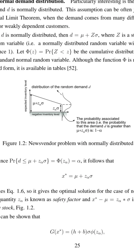
Normal demand distribution. Particularly interesting is the case when the demandd is normally distributed. This assumption can be often justified by the Central Limit Theorem, when the demand comes from many different indepen-dent or weakly depenindepen-dent customers.
Ifd is normally distributed, thend = µ+Zσ, whereZ is a standard normal random variable (i.e. a normally distributed random variable with mean 0 and variance 1). LetΦ(z) = Pr{Z < z} be the cumulative distribution function of the standard normal random variable. Although the functionΦis not available in closed form, it is available in tables [52].
zas negative inventory level
distribution of the random demand d
expected inventory level
m+zas
The probability associated to this area (i.e. the probability that the demand d is greater than
m+zas) is: 1-a
Figure 1.2: Newsvendor problem with normally distributed demand
SincePr{d≤µ+zασ}= Φ(zα) =α, it follows that
x∗ =µ+z
ασ
satisfies Eq. 1.6, so it gives the optimal solution for the case of normal demand. The quantity zα is known as safety factor and x∗ −µ = zα∗σ is known as the
safety stock, Fig. 1.2.
It can be shown that
whereφis the density function of the standard normal random variable, and that
π(x∗) = (p−c)µ−(p−s)σφ(zα).
In addition the fill-rate can be also easily written as
β= 1−cv[φ(zα)−(1−α)zα]
wherecv =σ/µis the coefficient of variation of the demand. Sinceφ(zα)−(1−
α)zα ≥ 0 is decreasing inα, it follows thatβ is increasing inα and decreasing
in cv. Notice, for example that β = 0.97 whenα = 0.75 and cv = 0.2, while
β = 0.991whenα = 0.9andcv = 0.2.
Example 1.2.4. Suppose thatdis normal with meanµ= 100and standard devi-ationσ = 20. Ifc = 5,h = 1andb = 3, thenα = b/(b+h) = 0.75andx∗ =
100 + 0.6745·20 = 113.49, in factΦ−1(0.75) ∼= 0.6745. Note that the order is for
13.49units (safety stock) more than the mean. Note also thatφ(0.6745) = 0.3178
soG(113.49) = 4·20·0.3178 = 25.42andπ(113.49) = 274.58, withβ = 0.97.
Inventory control policies. In the previous paragraph we introduced the Newsven-dor problem. The key aspect of this problem is the fact that a single replenishment decision concerning an order quantity has to be taken in advance, to meet the ran-dom demand till the end of the time horizon considered.
Nevertheless, what usually happens in the reality is that management has to take multiple decisions to meet the demand. These decisions usually concern the number of planned replenishments, the timing of such replenishments, and the quantity of items that has to be ordered at each replenishment. Obviously there are many different strategies to decide on replenishment periods and replenish-ment quantities. For instance we could fix a rule stating that a replenishreplenish-ment should be performed every time the inventory level falls below a given threshold. In this case the decision would concern two aspects: choosing the “threshold” and the quantity that has to be ordered when the inventory position falls below this threshold. Alternatively, a strategy could consist in ordering according to
prede-fined time intervals. Moreover, instead of deciding in advance the exact quantity to be ordered, we could instead try to fix a level for each replenishment (order-up-to-level) up to which we will raise the stocks. Each of these different strategies constitutes an inventory control policy.
For many replenishment policies a challenging problem is that of finding the optimal “settings”, for instance the reorder levels and the order-up-to-levels min-imizing some cost structure or meeting certain service level requirements [89]. Often people are also interested in comparing different policies in such a way to determine which policy always guarantees the best cost performance [76].
Notation and terminology. We shall now introduce some important issues and terminology concerning inventory control policies. When demand is stochas-tic, it is useful to conceptually categorize inventories as follows:
• On-hand stock: This is stock that is physically on the shelf; it can never
be negative. This quantity is relevant in determining whether a particular customer demand is satisfied directly from the shelf;
• Backorders: These denote an existing demand that cannot be fulfilled since
no stock is available on the shelf;
• On order: These are stocks which have been ordered, but that for some
reason have not reached the shelf yet. Reasons for this may comprise: stock inspection, transportation etc.;
• Net stock = (On hand) - (Backorders).
This quantity can become negative (namely, if there are backorders). It is used in some mathematical derivations and is also a component of the following important definition:
• Inventory position: The inventory position is defined by the relation
![Figure 2.2: In Tarim & Kingsman [89] the event that actual stock exceeds the order-up-to-level S n for a given review R n is assumed to be rare](https://thumb-us.123doks.com/thumbv2/123dok_us/10217065.2925549/84.918.194.726.220.886/figure-tarim-kingsman-event-actual-exceeds-review-assumed.webp)