Air Force Institute of Technology
AFIT Scholar
Theses and Dissertations Student Graduate Works
9-1-2018
Multi-Level Multi-Objective Programming and
Optimization for Integrated Air Defense System
Disruption
Aaron M. Lessin
Follow this and additional works at:https://scholar.afit.edu/etd
Part of theOperational Research Commons
This Dissertation is brought to you for free and open access by the Student Graduate Works at AFIT Scholar. It has been accepted for inclusion in Theses and Dissertations by an authorized administrator of AFIT Scholar. For more information, please [email protected]. Recommended Citation
Lessin, Aaron M., "Multi-Level Multi-Objective Programming and Optimization for Integrated Air Defense System Disruption" (2018).Theses and Dissertations. 1917.
MULTI-LEVEL MULTI-OBJECTIVE PROGRAMMING AND OPTIMIZATION FOR
INTEGRATED AIR DEFENSE SYSTEM DISRUPTION
DISSERTATION
Aaron M. Lessin, Major, USAF AFIT-ENS-DS-18-S-035
DEPARTMENT OF THE AIR FORCE AIR UNIVERSITY
AIR FORCE INSTITUTE OF TECHNOLOGY
Wright-Patterson Air Force Base, OhioDISTRIBUTION STATEMENT A
The views expressed in this document are those of the author and do not reflect the official policy or position of the United States Air Force, the United States Department of Defense or the United States Government. This material is declared a work of the U.S. Government and is not subject to copyright protection in the United States.
AFIT-ENS-DS-18-S-035
MULTI-LEVEL MULTI-OBJECTIVE PROGRAMMING AND OPTIMIZATION FOR INTEGRATED AIR DEFENSE SYSTEM DISRUPTION
DISSERTATION
Presented to the Faculty
Graduate School of Engineering and Management Air Force Institute of Technology
Air University
Air Education and Training Command in Partial Fulfillment of the Requirements for the Degree of Doctor of Philosophy in Operations Research
Aaron M. Lessin, BS, MS Major, USAF
September 2018
DISTRIBUTION STATEMENT A
AFIT-ENS-DS-18-S-035
MULTI-LEVEL MULTI-OBJECTIVE PROGRAMMING AND OPTIMIZATION FOR INTEGRATED AIR DEFENSE SYSTEM DISRUPTION
Aaron M. Lessin, BS, MS Major, USAF Committee Membership: Brian J. Lunday, PhD Chair Raymond R. Hill, PhD Member Kenneth M. Hopkinson, PhD Member Adedeji B. Badiru, PhD
AFIT-ENS-DS-18-S-035
Abstract
The U.S. military’s ability to project military force is being challenged. This dissertation develops, and demonstrates the application of, three respective sensor location, relocation, and network intrusion models to provide the mathematical basis for the strategic engagement of emerging technologically advanced, highly-mobile, Integrated Air Defense Systems. Herein, this research addresses each of these related problems via three distinct modeling and analysis efforts, each building upon the previous work.
First, a bilevel mathematical programming model is proposed for locating a het-erogeneous set of sensors to maximize the minimum exposure of an intruder’s pene-tration path through a defended region. This formulation also allows a defender to specify minimum probabilities of coverage for a subset of the located sensors (e.g., the most valuable sensors) and for high-value asset locations in the defended region. The bilevel program is reformulated to a single-level optimization problem for which instances can be readily solved using a commercial solver. Given the locations of a defender’s sensors, three alternative path identification models are formulated, each corresponding to conceptually-motivated intrusion-path metrics. A test instance is examined for the air defense of a border region against intrusion by an enemy air-craft; upon identifying the optimal, respective defender asset location and intruder routing solutions, intruder-optimal solutions corresponding to each of three alterna-tive metric-specific paths are examined, illustrating the relaalterna-tive impact of an intruder choosing an inappropriate metric. Sensitivity analyses are conducted to examine the effect of several model parameters on solution quality and required computational effort.
Next, consider a set of sensors having varying capabilities and respectively located to maximize an intruder’s minimal expected exposure to traverse a defended border region. Given two subsets of the sensors that have been respectively incapacitated or degraded, a multi-objective, bilevel optimization model is formulated to relocate surviving sensors to maximize an intruder’s minimal expected exposure to traverse a defended border region, minimize the maximum sensor relocation time, and minimize the total number of sensors requiring relocation. This formulation also allows the defender to specify minimum preferential coverage requirements for high-value asset locations and emplaced sensors. Adopting theε-constraint method for multi-objective optimization, a single-level reformulation is subsequently developed that enables the identification of non-inferior solutions on the Pareto frontier and, consequently, iden-tifies trade-offs between the competing objectives. The aforementioned model and solution procedure are demonstrated for a scenario in which a defender is relocating surviving air defense assets to inhibit intrusion by a fixed-wing aircraft.
Lastly, this research considers an attacker seeking an optimal intrusion path through a region defended by a sensor network, as measured by the expected exposure of the intruding attacker to the defender’s sensors. Herein, a trilevel mathematical programming formulation is presented in which an attacker respectively identifies a subset of the defender’s heterogeneous sensors to incapacitate and a subset of the de-fender’s network to degrade, subject to budget constraints; a defender subsequently relocates the surviving sensors, considering multiple, competing objectives; and in the third level, the attacker selects an optimal intrusion path to traverse through the defender’s sensor network. A bilevel reformulation is derived, new heuristics are devel-oped and tested, and the performance of the heuristics on synthetic-but-representative scenarios is reported.
AFIT-ENS-DS-18-S-035
To my Grandpa, my hero,
Acknowledgements
I would like to extend a sincere thank you to my advisor, Dr. Brian Lunday, for his unwavering support and guidance throughout this research. His passion for learning and pursuit of excellence has been a constant inspiration, and this work would not have been possible without his mentorship.
Thanks also to the other members of my research committee, Dr. Raymond Hill and Dr. Kenneth Hopkinson, for their support and assistance which helped bring this academic endeavor to fruition.
Table of Contents
Page Abstract . . . iv Acknowledgements . . . vii List of Figures . . . x List of Tables . . . xi I. Introduction . . . 1 1.1 Motivation . . . 11.2 Research Focus and Organization . . . 6
II. A Bilevel Exposure-oriented Sensor Location Problem for Border Security . . . 8
2.1 Introduction . . . 8
2.1.1 Literature Review . . . 10
2.1.2 Major Contributions and Organization . . . 16
2.2 Model & Methodology . . . 17
2.2.1 Assumptions . . . 17
2.2.2 Model . . . 19
2.2.3 Alternative Intrusion Paths . . . 25
2.3 Testing, Results, & Analysis . . . 31
2.3.1 Illustrative Instance for Air Defense of a Border Region . . . 31
2.3.2 Test Instance Generation . . . 33
2.3.3 Results . . . 35
2.3.4 Sensitivity Analysis . . . 39
2.4 Conclusions & Recommendations . . . 43
III. A Multi-objective, Bilevel Sensor Relocation Problem for Border Security . . . 45
3.1 Introduction . . . 45
3.1.1 Literature Review . . . 47
3.1.2 Major Contributions & Organization . . . 53
3.2 Model & Methodology . . . 54
3.2.1 Assumptions . . . 54
3.2.2 Model . . . 57
3.2.3 Methodology . . . 62
Page 3.3.1 Representative Scenario for Air Defense of a
Border Region . . . 65
3.3.2 Results . . . 69
3.3.3 Sensitivity Analysis . . . 77
3.4 Conclusions & Future Work . . . 80
IV. A Multi-objective, Trilevel Sensor Network Intrusion Problem . . . 83
4.1 Introduction . . . 83
4.1.1 Literature Review . . . 85
4.1.2 Major Contributions & Paper Organization . . . 92
4.2 Model & Methodology . . . 93
4.2.1 Assumptions . . . 94
4.2.2 Model Formulation . . . 97
4.3 Heuristic Solution Methods . . . 105
4.3.1 Heuristic 1 (H1): Piecewise incapacitation and degradation strategy determination . . . 105
4.3.2 Heuristic 2 (H2): Sequential incapacitation and degradation strategy determination . . . 113
4.4 Testing, Results, & Analysis . . . 115
4.4.1 Representative Scenario for the Intrusion of an Air Defense Network . . . 115
4.4.2 Results . . . 120
4.5 Conclusions & Recommendations . . . 125
V. Conclusion . . . 127
5.1 Contributions . . . 127
5.2 Recommendations for Future Research . . . 129
Appendix A. 2018 WDSI Proceedings: A Multi-objective Bilevel Optimization Model for the Relocation of Integrated Air Defense System Assets . . . 132
List of Figures
Figure Page
1 Hexagonal tessellation example . . . 19
2 Probability-of-kill curve for each SAM battery type . . . 33
3 Baseline Maximin Exposure Problem solution . . . 35
4 Exposure values by path edge for four alternative intrusion paths . . . 38
5 Probability-of-kill curve for each SAM battery type . . . 67
6 Initial IADS layout . . . 69
7 Initial IADS layout before asset relocations showing incapacitated and degraded assets . . . 70
8 Multi-Objective Sensor Relocation Problem solution with ε2, ε3 unrestricted . . . 71
9 Optimal minimal exposure values for discretized (ε2, ε3)-combinations . . . 72
10 Percentage of maximum recoverable minimal exposure achievable for (ε2, ε3)-combinations . . . 74
11 Pareto optimal relocation solution with (ε2, ε3) = (1,1) . . . 76
12 Pareto optimal relocation solution with (ε2, ε3) = (2.5,4) . . . 77
13 Effect of SAM battery spacing level on problem size. . . 79
14 Effect ofdhex and ABR onLBhex. . . 80
15 Initial IADS layout . . . 117
16 Heuristic 1 solution to Instance 3 . . . 122
17 Heuristic 1 solution to Instance 2 . . . 124
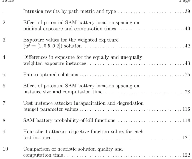
List of Tables
Table Page
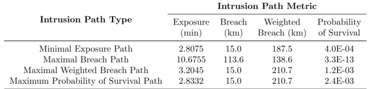
1 Intrusion results by path metric and type . . . 39 2 Effect of potential SAM battery location spacing on
minimal exposure and computation times . . . 40 3 Exposure values for the weighted exposure
(wt = [1,0.5,0.2]) solution . . . 42
4 Differences in exposure for the equally and unequally
weighted exposure instances . . . 43 5 Pareto optimal solutions . . . 75 6 Effect of potential SAM battery location spacing on
instance size and computation time. . . 78 7 Test instance attacker incapacitation and degradation
budget parameter values . . . 116 8 SAM battery probability-of-kill functions . . . 118 9 Heuristic 1 attacker objective function values for each
test instance . . . 121 10 Comparison of heuristic solution quality and
MULTI-LEVEL MULTI-OBJECTIVE PROGRAMMING AND OPTIMIZATION FOR INTEGRATED AIR DEFENSE SYSTEM DISRUPTION
I. Introduction
1.1 Motivation
A key to the United States military’s overwhelming historical success is due in large part to its ability to achieve and maintain air superiority. For the past half century, the United States has conducted combat operations relatively unimpeded, projecting power across the globe at will. However, this level of success has not gone unnoticed, and enemy nations have been forced to reassess their strategies in hope of achieving future success. As a result, many nations have adopted an antiaccess/area-denial (A2/AD) strategy to inhibit the United States’ ability to penetrate their borders and project military power.
Unfortunately, past performance does not guarantee future success for the United States military. The operational environment is changing, and the United States’ future military success will also depend on its own ability to adapt. This level of con-cern has risen to the highest ranks within the U.S. Air Force. In August 2016, during his “State of the Air Force” address, Air Force Chief of Staff General David Goldfein expressed his concern, stating that “air superiority is not an American birthright. It’s actually something you have to fight for and maintain” (Goldfein & James, 2016).
Current U.S. doctrine for the suppression of enemy air defenses (SEAD) in Joint Publication (JP) 3-01, Countering Air and Missile Threats (specifically, Chapter 4, “Offensive Counterair Planning and Operations”) highlights the need for a serious
reassessment of our strategy. JP 3-01 acknowledges that “potential adversaries’ IADS [Integrated Air Defense Systems] have become increasingly complex and needs to be analyzed in-depth with an eye to potential strengths and weaknesses” (United States Joint Chiefs of Staff, 2012b). The document also discusses the change in mobility and effectiveness of enemy IADS as compared to past technologies. “SAM [Surface to Air Missile] forces have become more mobile and lethal, with some systems demonstrating a ‘shoot-and-move’ time in minutes rather than hours or days” (United States Joint Chiefs of Staff, 2012b). Although current doctrine recognizes the emergence of a more effective, modern A2/AD threat, JP 3-01 fails to provide a comprehensive approach to defeat such a threat.
In its section on “Suppression of Enemy Air Defenses,” JP 3-01 details three cate-gories of SEAD execution, namely (1) area of responsibility/joint operations area-wide (AOR/JOR-wide) air defense (AD) system suppression, (2) localized suppression, and (3) opportune suppression. AOR/JOR-wide air defense system suppression targets “high payoff AD assets that result in the greatest degradation of the enemy’s to-tal system,” focusing on the destruction of “key C2 [Command and Control] nodes” (United States Joint Chiefs of Staff, 2012b). Unfortunately, enemy IADS command and control networks are becoming highly dispersed, decentralized, and redundant. Therefore, this category of SEAD execution will become much less effective in the future. The second category of SEAD, localized suppression, is focused on escort operations that are “normally confined to geographic areas associated with specific targets or transit routes for a specific time” (United States Joint Chiefs of Staff, 2012b). Under this category are two subcategories - planned localized suppression and immediate localized suppression. Planned localized suppression is a bottom-up, reactive approach whereby “localized suppression requests are processed from the lowest echelon of command to to the highest using the appropriate air control
sys-tem” (United States Joint Chiefs of Staff, 2012b). Immediate localized suppression is similar to its counterpart except with the added necessity of an immediate response, “similar to immediate requests for CAS [Close Air Support]” (United States Joint Chiefs of Staff, 2012b). It is clear that both subcategories of localized suppression are highly reactive as opposed to a deliberate, offensive approach. The final category of SEAD, opportune suppression, is also “unplanned and includes aircrew self-defense and attack against surface-AD targets of opportunity” (United States Joint Chiefs of Staff, 2012b). Included under the opportune suppression category of SEAD are also the following four subcategories: aircrew self-defense, targets of opportunity, targets acquired by observers or controllers, and targets acquired by aircrews. Again, a com-mon theme characterized by a defensive and reactive strategy is present, complicated by the “proliferation of highly mobile AD weapon systems, coupled with deception and defensive tactics” (United States Joint Chiefs of Staff, 2012b).
Recognizing the gap in U.S. doctrine for defeating an ever developing and in-creasingly modern IADS threat, Lt Elliot Bucki recently proposed the addition of a new category of SEAD, termed “planned opportune suppression” (Bucki, 2016). This category of SEAD would combine the “planned nature of localized suppression and the tactics of opportune suppression” to produce a strategy that is more offensive-minded and proactive as opposed to the current doctrine which is more defensive and reactive (Bucki, 2016). This strategy makes three key assumptions about the nature of the new IADS threat which helps focus and shape its approach. First, it assumes that “almost all IADS components will be mobile and linked together in a system with considerable redundancy” (Bucki, 2016). Second, it assumes that non-stealth aircraft or those aircraft not equipped with long range standoff weapons will be “out-ranged” by technologically advanced IADS threats (Bucki, 2016). Third, it assumes that modern IADS will be “inherently resistant to jamming and electronic attack”
(Bucki, 2016). All of these assumptions help provide a realistic assessment of the modern IADS threat the U.S. is certain to face in an A2/AD environment.
It is important to note that Bucki’s SEAD category of planned opportune suppres-sion also accounts for the important temporal aspect in engaging an enemy IADS. By adding planned opportune suppression to JP 3-01, U.S. SEAD doctrine would con-tain a proactive approach that offers flexibility in attacking a highly mobile enemy IADS threat, providing a strategy that focuses on “planned on-call targets,” while still offering the necessary flexibility to handle time critical targets of opportunity (United States Joint Chiefs of Staff, 2012b).
There has also been recent doctrinal development on the part of the Joint Chiefs of Staff as found in their “Joint Operational Access Concept (JOAC)” (United States Joint Chiefs of Staff, 2012a). Recognizing the “dramatic improvement and prolifer-ation of weapons and other technologies,” the document proposes a new concept for achieving operational access against an increasingly capable enemy that has adopted an antiaccess/area-denial strategy (United States Joint Chiefs of Staff, 2012a). Op-erational access is defined as “the ability to project military force into an opOp-erational area with sufficient freedom of action to accomplish the mission” (United States Joint Chiefs of Staff, 2012a). The JOAC doctrine notes that “the ability to ensure oper-ational access in the future is being challenged - and may well be the most difficult operational challenge U.S. forces will face over the coming decades” (United States Joint Chiefs of Staff, 2012a).
In order to combat this emerging threat, the document lists multiple precepts de-scribing how future joint forces could achieve operational access in the face of armed opposition. Some suggestions include: (1) “conduct operations based on the require-ments of the broader mission, while also designing subsequent operations to lessen access challenges, (2) seize the initiative by deploying and operating on multiple,
inde-pendent lines of operations, (3) create pockets or corridors of local domain superiority to penetrate the enemy’s defenses and maintain them as required to accomplish the mission, (4) maneuver directly against key operational objectives from strategic dis-tance, (5) attack enemy antiaccess/area-denial defenses in depth rather than rolling back those defenses from the perimeter, and (6) maximize surprise through deception, stealth, and ambiguity to complicate enemy targeting” (United States Joint Chiefs of Staff, 2012a). This verbiage is strikingly different than the current SEAD doctrine found in JP 3-01. Here, a set of precepts outlines the development of a comprehen-sive operational concept for conducting planned, offencomprehen-sive operations in support of achieving the broader strategic objectives in a highly contested A2/AD environment. In order to aid counter-A2/AD efforts, the JOAC recommends that future joint forces leverage “cross-domain synergy - the complementary vice merely additive em-ployment of capabilities in different domains such that each enhances the effectiveness and compensates for the vulnerabilities of the others - to establish superiority in some combination of domains that will provide the freedom of action required by the mis-sion” (United States Joint Chiefs of Staff, 2012a). Whereas synergy between joint forces has historically been a U.S. military strength, the unity of effort required for cross-domain synergy will require a higher level of integration, acting across domains and at lower echelons. This will allow the joint forces to exploit “fleeting local op-portunities for disrupting the enemy system” because the temporal aspect of warfare will be critical in achieving cross-domain success. The days of overwhelming air supremacy will be far less likely, and air superiority as mentioned in the JOAC may not be “widespread or permanent; it more often will be local and temporary” (United States Joint Chiefs of Staff, 2012a).
1.2 Research Focus and Organization
Although the U.S. has taken significant steps in identifying the gaps in doctrine and proposing concepts for confronting a highly mobile, technologically advanced A2/AD enemy threat, the greater difficulty will be in operationally implementing these new concepts. This research provides a mathematical lens to analyze the emerg-ing A2/AD threat with the aim of understandemerg-ing how to engage and defeat future adversaries. To accomplish this task, this dissertation focuses on three main avenues of research, each building upon the previous work.
To ultimately defeat an advanced A2/AD threat, it is critical to first understand how an enemy may construct (i.e., layout) an air defense network consisting of a set of ground-based air defense assets to prevent intrusion of a defended region. To wit, Chapter II presents a bilevel math programming model to determine the optimal layout of a given set of heterogeneous assets to maximize the minimum exposure of an intruder’s penetration path through a defended border region.
Considering the rapid increase in air defense asset mobility, it is also important to determine how an enemy may reposition surviving ground-based IADS assets fol-lowing an attack. Given two subsets of the assets that have been respectively inca-pacitated or degraded, Chapter III formulates a multi-objective, bilevel optimization model to relocate surviving assets to maximize an intruder’s minimal expected ex-posure to traverse a defended border region, minimize the maximum asset relocation time, and minimize the total number of assets requiring relocation.
Once a better understanding has been achieved regarding how an enemy may optimally locate and relocate ground-based elements of an A2/AD IADS, the research herein shifts its focus to the ultimate goal of the dissertation - determining how to optimally attack and penetrate an enemy air defense system. To accomplish this, Chapter IV proposes a trilevel mathematical programming formulation in which an
attacker respectively identifies a subset of the defender’s heterogeneous sensors to incapacitate and a subset of the defender’s network to degrade, subject to budget constraints; a defender subsequently relocates their sensors to maximize the attacker’s minimal exposure, minimize the maximum relocation time, minimize the maximum number of sensors requiring relocation, and minimize the under coverage of high-value assets and emplaced sensors; in the third level, the attacker selects an optimal intrusion path through the defender’s sensor network.
For each of the three main research efforts presented in Chapters II, III, and IV, detailed solution techniques are presented, and their application is demonstrated via a representative air defense scenario. A discussion of selected analyses is also provided therein. Chapter V concludes with a summary of the contributions and recommendations for future research.
By accomplishing each of these research goals, this dissertation provides a basis for the operational implementation of the concepts outlined in the JOAC and the proposed improvements to JP 3-01 to provide the strategic planning that will be necessary to effectively engage and defeat the emerging A2/AD IADS threat.
II. A Bilevel Exposure-oriented Sensor Location Problem
for Border Security
2.1 Introduction
National, group, and individual sovereignty requires protection against threats. At the national level, potential threats include the illegal or unauthorized movement of people, weapons, or drugs. At the group level, corporations seek to defend their computer networks against malicious code. Individual sovereignty concerns include protection of a residence against burglary. The defense against such threats begins at a border or boundary of the region under a defender’s control, whether it be physical or virtual. Moreover, the defense against threats occurs within a border region, wherein a defender will locate and use assets to detect and/or interdict a would-be intruder.
Evidence of the growing requirement for border security can be seen in a 2017 memorandum from the U.S. Department of Homeland Security (DHS) which indi-cates “the surge of illegal immigration at the southern border has overwhelmed federal agencies and resources and has created a significant national security vulnerability to the United States” (Kelly, 2017). As a result, the U.S. House of Representatives Homeland Security Committee passed a $10 billion bill (McCaul, 2017) to “deter, impede, and detect illegal activity” through the use of integrated surveillance and intrusion detection assets such as the Integrated Fixed Tower (IFT) System and the Remote Video Surveillance System (RVSS). IFTs are fixed sensors that provide long-range, persistent surveillance by automatically detecting and tracking targets of interest. Similarly, RVSS assets are fixed sensors that use cameras, radio, and mi-crowave transmitters to “provide short-, medium-, and long-range persistent surveil-lance mounted on stand-alone towers, or other structures” (Alles et al., 2016). The bill also sets aside $10 million to implement Vehicle and Dismount Exploitation Radars
(VADER) in border security operations (McCaul, 2017). Since 2006, unmanned sys-tems equipped with VADER sensors have been credited with interdicting over “13,144 pounds of cocaine and 321,330 pounds of marijuana worth an estimated $1.8 billion” (Alles et al., 2016).
Oriented against aerial threats to border security, ground-based air defense weapons are emplaced as part of an antiaccess/area-denial (A2/AD) strategy to defend against enemy aircraft attempting to penetrate a country’s border region during active con-flict. Many countries have adopted A2/AD strategies (Schmidt, 2016) and signif-icantly advanced their Surface to Air Missile (SAM) technology. Over the last 10 years, Russia has developed and fielded the S-400 Triumf air defense weapon system which can destroy aerial targets at ranges of 40-400 km (Foss & O’Halloran, 2014). This highly-effective SAM system is capable of engaging the world’s most premier aircraft, as well as cruise missiles and ballistic missiles. Recent reports indicate the Russian military currently operates 39 S-400 battalions, with each battalion consisting of eight launchers and up to 112 missiles, along with radar systems and a command post (Gady, 2017). China, Turkey, India, and Saudi Arabia have all signed contracts for the purchase of multiple S-400 systems from Russia (TAS, 2017). Motivated by this trend in air defense posturing, in this study we construct an air defense test instance as an illustrative border security application.
Border security is no longer limited to physical borders but now includes virtual, software-defined borders, creating vulnerabilities from the economic market to the energy sector. Due to recent threats “targeting government entities and organizations in the energy, nuclear, water, aviation, and critical manufacturing sectors” the DHS and the Federal Bureau of Investigation (FBI) released an alert “to educate network defenders and enable them to identify and reduce exposure to malicious activity” (DHS, 2017). This emerging threat is not simply a U.S. problem; in December 2015,
a cyberattack on the Ukrainian power grid left over 225,000 people without power (Lee et al., 2016). Daniel Tobok, CEO and co-owner of Toronto-based Cytelligence, estimates that cyberattacks “cost Canada $3 billion to $5 billion per year in proceeds to criminals, adding one Calgary energy company was forced to pay $200,000 in ransom three years ago to regain control of its corrupted digital production systems” (Healing, 2017). In his 2017 State of the Union Address, European Commission President Jean-Claude Juncker said that “cyber-attacks can be more dangerous to the stability of democracies and economies than guns and tanks” (Juncker, 2017).
Common to each of these border security applications is that a defender must decide where to locate a set of assets to prevent an adversary from traversing through a region; the defender’s assets may also have differing capabilities to detect or en-gage the adversary; some defensive assets may be important enough to the defender because of their high cost or limited supply to warrant protection, once emplaced; specific locations of the defended region may require preferential coverage due to their importance; and an adversary will be able to observe the location of defender assets and select a route through the border region to minimize their likelihood of detection.
2.1.1 Literature Review.
Our modeling efforts for this research focus on implementing and extending pre-vious work in facility location. Schilling et al. (1993) presented a detailed overview of covering problems in facility location. They classified models as either a Set Covering Problem (SCP) or a Maximal Covering Location Problem (MCLP), where coverage is either required or optimized, respectively. The MCLP was first introduced by Church & ReVelle (1974) to maximize the amount of demand covered within a spec-ified service distance by locating a fixed number of facilities. White & Case (1974) extended the work of Church & ReVelle (1974) by considering equal weights on all
demand points. Church (1984) later introduced the MCLP on a planar surface using Euclidean and rectilinear distance measures, where potential facility locations are no longer discrete (and finite).
One of the main assumptions of the MCLP is that coverage is binary. That is, a demand point is either fully covered or not covered at all by a located facility. However, this assumption is often unrealistic. Berman & Krass (2002) extended the MCLP to the Generalized Maximal Covering Location Problem (GMCLP), allowing for “partial coverage of customers, with the degree of coverage being a non-increasing step function of the distance to the nearest facility.” Additionally, Berman et al. (2003) extended the GMCLP by way of a gradual covering decay model. Drezner et al. (2004) also solved the gradual covering problem on a planar surface.
Traditional facility location models do not address the need to prevent the passage of an adversary into friendly territory, which is the main concern for border security applications. However, a related field of research pertaining to the location of sensors in a Wireless Sensor Network (WSN) presents coverage models designed specifically for such a purpose. One of the three main coverage problems discussed in WSNs is
barrier coverage (Cardei & Wu, 2006). In the context of WSNs, “a given belt region is said to be k-barrier covered with a sensor network if all crossing paths through the region are k-covered, where a crossing path is any path that crosses the width of the region completely” (Kumar et al., 2005). A path is said to bek-covered if it intersects at least k sensors’ sensing ranges (Huang & Tseng, 2005).
As the defender, the goal of a barrier coverage model is to locate a set of sensorsS
such that some chosen measure of coverage is maximized. Alternatively, an attacker seeks to interdict or locate areas of the region where the value of the coverage measure is minimized. One such measure of coverage often used in WSN models is exposure. First introduced by Meguerdichian et al. (2001), exposure can informally be thought
of as the “expected average ability of observing a target in the sensor field.” More formally, exposure is defined as “an integral of a sensing function that generally depends on distance from sensors on a path from a starting point pS to destination
point pD” (Meguerdichian et al., 2001). Unlike some coverage metrics, the element
of time is important for exposure, since the ability of a sensor to detect a target can improve as the sensing time (i.e., exposure) increases.
For a sensor s, the general sensing model S at an arbitrary point p is:
S(s, p) = λ
[d(s, p)]K, (1)
where d(s, p) is the Euclidean distance between the sensor s and the point p, and positive constants λ and K are technology-dependent parameters (Meguerdichian et al., 2001). The parameter λ can be thought of as the energy emitted by a target, and K is an energy decay factor, typically ranging from 2 to 5 (Amaldi et al., 2008). The exposure of an object in the sensor field during the interval [t1, t2] along the
path p(t) is defined by Meguerdichian et al. (2001) as:
E(p(t), t1, t2) = Z t2 t1 I F, p(t) dp(t) dt dt, (2)
wherein the sensor field intensityI F, p(t) is implemented using anAll-Sensor Field Intensity model or aClosest-Sensor Field Intensity model, depending on the applica-tion and types of sensors used. TheAll-Sensor Field Intensity model is a summation of the sensing function values (1) from target p to all sensors in the sensor net-work, defined asIA(F, p) =Pn
i=1S(si, p), whereas theClosest-Sensor Field Intensity
model only utilizes the sensing function value of the closest sensor to the target (Meguerdichian et al., 2001).
algo-rithm to find the minimal exposure path in a sensor network. The algorithm first transforms the problem into a discrete domain utilizing a generalized grid approach and then creates an edge-weighted graph. The algorithm then applies Dijkstra’s single-source shortest-path algorithm (Dijkstra, 1959) to find the minimal exposure path from the source point pS to the destination point pD. Meguerdichian et al.
(2001) also extended this initial work by developing a localized minimal exposure path algorithm using Voronoi diagrams.
Understanding that signals traveling from a target to a sensor are often corrupted by noise, Clouqueur et al. (2002) added an Adaptive White Gaussian Noise term
Ni, i = 1, ..., n, to the initial sensor model in Equation (1). Clouqueur et al. (2002)
also presented the concepts of value fusion and decision fusion as alternative tech-niques for collaborating sensors to decide whether a target is actually present in the field to avoid false alarms. In the same paper, Clouqueur et al. (2002) developed a multi-phase random deployment strategy to minimize the cost of sensor deployment while achieving a desired detection performance. Adlakha & Srivastava (2003) deter-mined the minimum number of randomly deployed sensors required to guarantee a given exposure level. Veltri et al. (2003) presented a localized algorithm that enables a sensor network to determine its minimal exposure path. More recently, Amaldi et al. (2008) formulated two exposure-based optimization problems to respectively minimize the number of sensors required while guaranteeing a minimum exposure and, alternatively, to maximize the exposure of the least exposed path subject to a budget constraint on the sensors’ installation cost. Tian et al. (2014) presented a motion-planning scheme to direct the movement of mobile sensors for better detect-ing “smart” intruders. Lastly, Feng et al. (2016) proposed a minimal exposure path problem that requires the passage of a path around the boundary of an inaccessible region, and is solved using a hybrid genetic algorithm.
Another metric used to evaluate the quality of service provided by a WSN is
maximal breach, first proposed by Meguerdichian et al. (2001). Given a field A with
n sensorssi ∈S ={1, ..., n} located at (xi, yi), let pointsI and F be initial and final
locations, respectively, of an intruder traveling throughA. Given a pathP connecting
I to F, breach is defined as the minimum Euclidean distance from P to any sensor in S (Megerian et al., 2005). Furthermore, among all possible paths connecting I
and F, the path that has the maximum breach value is called the maximal breach path, PB (Duttagupta et al., 2007). For an intruder, thebreach of PB represents the closest the intruder will be to any sensor in A when traveling from point I to F. For the defender, breach represents how close to a sensor the intruder is guaranteed to travel, no matter which path the intruder traverses through the field for a given sensor layout.
In many WSN models wherein the objectives involve partial, if not complete, cov-erage of all grid points, the number of sensors available for deployment is typically not limited. However, in some situations resources may be limited and must be optimally allocated across a vast geographical area. WSN algorithms that make use of Voronoi diagrams and breach values are often better suited for this purpose. Meguerdichian et al. (2001) demonstrated how the critical edges of a maximal breach path could be used as a guide for determining where to add sensors in order to improve overall cover-age. Duttagupta et al. (2007) developed a sensor insertion-based heuristic procedure to achieve the maximum possible improvement in average breach. This procedure provides an approach that builds up a sensor network by successively adding sensors to reduce the breach value as much as possible. Cavalier et al. (2007) presented a heuristic based on Voronoi diagrams to locate a finite number of sensors to detect an event in a given planar region where the objective is to minimize the maximum prob-ability of non-detection. Recently, Karabulut et al. (2017) presented a mixed-integer
linear bilevel programming formulation, called the Maximal Breach Path Coverage Problem (MBPCP), along with three Tabu search heuristics; the defender determines the best sensor locations to maximize security, and the intruder reacts by destroying a subset of the sensors to increase the probability of evading detection, as computed using a maximal breach path approach.
There are several important distinctions that should be made between minimal exposure and maximal breach coverage models. Exposure models incorporate the element of time, assuming that sensors are more likely to detect an intruder given a longer period of observation. The minimal exposure problem seeks a path between pointspSandpDsuch that thetotal exposure acquired from the sensors by the moving
target is minimized. Alternatively, the maximal breach problem seeks a path from point pS topD such that the maximum exposure to the sensors at any given point is
minimized (Veltri et al., 2003). This is a key distinction between the two approaches. In terms of exposure, it may be beneficial to move closer to a sensor for a period of time to shorten the total path length and decrease the total exposure.
From the defender’s perspective, our goal is to determine the optimal sensor lay-out to prevent an intruder from crossing a defended region of interest. We employ a minimal exposure path approach, and our objective is to maximize the intruder’s min-imal exposure. We are not concerned with forcing a specified probability of coverage during at least one segment of the intrusion path, but we instead seek to maximize the intruder’s total exposure across the entire path. If we were to adopt a maximal breach path approach to solve this problem, our objective would be to minimize the intruder’s maximal breach. That is, we would want to guarantee that, at some point in the traversal of the defended region, the intruder is within a certain distance of a sensor. However, it is unlikely, if not impossible, that we could force an intruder to always be within the coverage range across the entire space; we would be seeking to
ensure at least one opportunity exists for which the intruder is within the coverage range of a sensor. As the defender, an exposure-based approach may offer many more opportunities to engage an intruder relative to a maximal breach path approach.
2.1.2 Major Contributions and Organization.
A majority of the research implementing breach- and exposure-coverage metrics focuses on determining the maximal breach path or calculating the minimal exposure path for a given sensor layout. Our chief concern, however, is to find the optimal de-ployment of a given set of sensors to maximize the minimal exposure of an intruder’s traversal of a defended region. Extending the work of Amaldi et al. (2008), this paper develops the notion of weighted exposure, considering a set of heterogeneous sensor types. The exposure weights represent the defender’s sensor preferences in terms of which sensors the defender prefers to employ when interdicting the intruder. Our formulation also allows the defender to specify required minimum probabilities of coverage for a subset of the located sensors (e.g., the most valuable sensors) and for high-value asset locations in the defended region (e.g., fielded force locations, popu-lation centers, command and control centers, etc.), balancing the exposure objective with the protection of sensors and high-value asset locations. We also demonstrate the robustness of the exposure metric for border protection by formulating and analyzing three additional alternative intrusion path metrics. That is, the optimal objective value of the minimal exposure solution results in the worst-case exposure of an in-truder’s traversal of the defended region, regardless of the inin-truder’s chosen metric for intrusion path determination.
Section 2.2 presents the bilevel mathematical formulation for solving the sen-sor location problem as well as a single-stage reformulation, and it proposes three conceptually-motivated, alternative intrusion path metrics an intruder might
con-sider adopting. Section 2.3 provides a military air defense scenario as an illustrative example for the application of the model, and it details the test instance generation, presents solutions, and provides sensitivity analysis results. Section 2.4 concludes with a summary of our findings and recommendations for future research.
2.2 Model & Methodology
In this section, we present a baseline formulation for the optimal sensor location problem, extending a modeling approach presented by Amaldi et al. (2008) wherein the authors seek to maximize the exposure of the least exposed path subject to a budget on the sensor installation cost. Unlike Amaldi et al. (2008), our model includes a heterogeneous set of sensors, and we introduce the notion of weighted exposure, allowing for defender-specified preferences between sensor types. We also add constraints to ensure defender-specified minimum probabilities of coverage for a set of high-value asset locations the defender seeks to protect. Considering instances where the loss of a sensor is highly undesirable, we include additional constraints to provide minimum probabilities of coverage for located sensors, by sensor type. Therefore, given a specified set of heterogeneous sensors, we determine the optimal layout that maximizes the minimal expected exposure of an intruder attempting to traverse the region, while ensuring adequate coverage of emplaced sensors and high-value asset locations.
2.2.1 Assumptions.
We make several assumptions related to the defender’s objectives and sensors. Regarding the objectives, we assume that, in addition to constructing a sensor network to inhibit an adversary traversing the defended region, the defender also wants to provide specific coverage of a set of high-value asset locations (e.g., population centers,
command and control centers, etc.) and a subset of the located sensors (e.g., the most valuable sensors). A minimum probability of protection is specified for each high-value asset location of interest and for each sensor type. The overall objective is to determine the location of sensors to maximize the ability to intercept intruding targets while protecting the high-value asset locations and a subset of the located sensors.
In many instances, points within a sensor coverage ring are not fully covered, whereas points outside remain completely uncovered. Rather, a probability of cov-erage exists for a target located at a given distance from a sensor location. As the distance from target to sensor decreases, the probability of coverage increases. In-stead of assuming binary sensor coverage (i.e., covered/not covered), we implement a probability-of-coverage curve as a function of the distance from target to sensor, for each of the heterogeneous sensor types. Furthermore, we assume the defender’s incoming threat is a single target with a specified constant velocity.
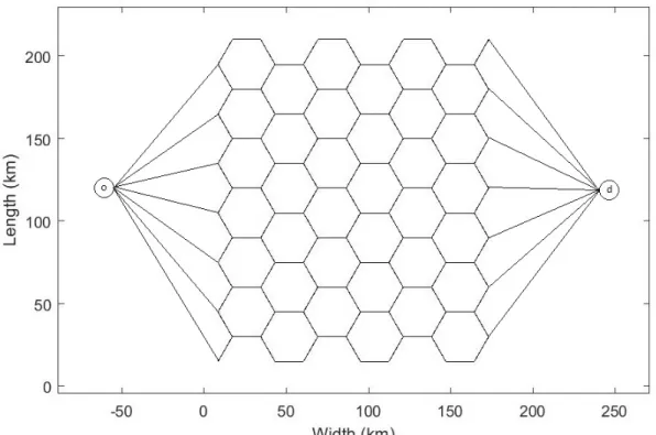
To formulate instances of our model, we construct a hexagonal tessellation over the border region of interest, as shown in Figure 1. The intruding target traverses the arcs of the graph, traveling from artificial origination node o on the left side of the hexagonal grid to the artificial destination node d on the right. Potential sensor locations are positioned at the center of each hexagon in the grid. We choose to discretize the border region using a mesh of uniformly-sized regular hexagons, as Yousefi & Donohue (2004) demonstrated it to be superior to alternative uniform tessellation means (e.g., square, rhombus, triangle) as it provides more freedom of movement for the intruder.
Lastly, we assume the adversaries know each others’ capabilities, and the intruder has sufficiently capable intelligence to know the defender’s sensor locations.
Figure 1. Hexagonal tessellation example
2.2.2 Model.
The following list of sets, parameters, and decision variables are used to formulate the mathematical programming models considered herein.
Sets:
T : the set of all types of sensors available to locate, indexed by t.
S : the set of all sites where sensors can be located, indexed bys.
F : the set of all sites where high-value assets are located, indexed byf.
A : the set of arcs over which an intruding target can traverse, indexed by (i, j).
N : the set of all nodes at which arcs intersect and through which an intruding target can traverse, indexed byn.
G= (N, A) : the graph over which an intruding target will traverse, as induced by the set of potential sensor sitess ∈S.
Parameters:
wt : the exposure weight for sensor type t∈T.
est
ij : the exposure time of a target traversing arc (i, j)∈A to a sensor
of typet ∈T located at site s∈S.
Bt : the maximum number of type t∈T sensors available to locate.
pt
sp : the probability that a sensor of typet ∈T located at site s∈S
can cover the point p.
Cf : the minimum probability of coverage required for each high-value
asset location f ∈F.
Ct: the minimum probability of coverage required for each located sensor of typet ∈T.
Decision Variables:
xts : 1 if the defender locates a type t∈T sensor at sites ∈S, and 0 otherwise.
yij : 1 if the intruder traverses arc (i, j)∈A, and 0 otherwise.
Given our assumptions, the game theoretic view of this problem is that of a two-player, extensive-form, two-stage, zero-sum game with perfect and complete in-formation. In the upper-level problem, the defender determines the locations of a set of heterogeneous sensors. Observing this decision, the intruder reacts in the lower-level problem by selecting arcs to traverse the region. The defender and intruder seek
to respectively maximize and minimize the total expected weighted exposure of the least exposed path. Leveraging the aforementioned notation, we formulate the bilevel
Maximin Exposure Problem (MmEP) corresponding to this Stackelberg game as follows: MmEP: max x miny X (i,j)∈A X s∈S X t∈T wtestijxts yij (3) s.t. X s∈S xts=Bt, ∀t ∈T, (4) X t∈T xts≤1, ∀s∈S, (5) X s∈S X t∈T ln 1−ptsf xts ≤ln 1−Cf , ∀f ∈F, (6) X s∈S\{s¯} X t∈T ln1−ptss¯xts ≤ln1−Ctxt¯s, ∀s¯∈S, t∈T (7) X j:(i,j)∈A yij− X j:(j,i)∈A yji = 1, i=o, −1, i=d, 0, i=N \ {o, d}, ∀i∈N, (8) yij ≥0, ∀(i, j)∈A, (9) xts∈ {0,1}, ∀s ∈S, t∈T. (10)
The objective function (3) maximizes the total expected weighted exposure of the intruder’s minimal exposure path, where P
s∈S P t∈T
wtestijxts represents the expected weighted exposure of a target traversing a given arc (i, j) ∈ A to sensors of type
t ∈ T emplaced (i.e., xt
s = 1) at locations s ∈ S. The exposure weights wt account
for the defender’s preferences of sensors for engaging the intruder. We propound that cardinality weighting is appropriate for most applications, as it results in an objec-tive calculation of exposure times for an intruder. However, we retain the general
model havingwt-parameters for a special case wherein the defender may exhibit
pref-erences over the sensor types t ∈ T. As a defender-focused model, the purpose of these weights is to determine the optimal location of the sensors,given the defender’s sensor preferences. For a given set ofwt-parameter values, the resulting formulation
corresponds to the framework of a zero-sum game with perfect and complete infor-mation. Were the intruder to assume any other set of weights than the actual ones adopted by a defender, a different intrusion path may result; however, such a different path can only yield a better objective function value for the defender. If the intruder does perceive the defenders priorities correctly, the optimal solution identified via our model represents the worst-case solution from the defender’s perspective.
For example, the defender could specify exposure weights of 1.0, 0.5, and 0.2 for a model with three different sensor types. For such a case, the defender would prefer to use the first sensor type over all other sensor types to engage the intruder. Alterna-tively, exposure weights may be parameterized to account for qualitative differences in sensor effectiveness not captured by the quantitative differences inherent in the sensor probability functions. Qualitative differences in sensor performance may re-sult from factors such as insufficient sensor operator training or operational technical complexity of a given sensor type. Under this interpretation, the defender may be half as effective at employing the second type of sensor against a target compared to using the first sensor type.
Constraint (4) specifies the number of each type of sensor the defender can locate. Constraint (5) prevents more than one sensor from being located at the same site. Constraint (6) ensures that all high-value asset locations receive the required coverage. The form of Constraint (6) results from a logarithmic transformation of the constraint
1−Y s∈S Y t∈T 1−ptsf xt s ≥Cf, ∀f ∈F, (11)
wherein independence is assumed among the probabilities of coverage,pt
sf over sensor
locations, s ∈ S, and sensor types, t ∈ T. (Implied is the assumption that Cf <1,
which is appropriate for this probabilistic metric wherein certain coverage is not attainable.) Likewise, Constraint (7) provides for the coverage of emplaced sensors by other sensors, as may be required by specific applications to protect valuable sensors. That is, for every site ¯s∈S, if a defender locates a sensor of typet∈T (i.e.,xts¯= 1), Constraint (7) requires a specified level of coverage,Ct, via the effects ofother sensors the defender chooses to locate (i.e., xts,∀s∈S\ {s¯}). In contrast, if a defender does not locate a sensor of type t ∈ T at a site ¯s ∈ S (i.e., xt
¯
s = 0), then the constraint
effectively requires at least Ct = 0 (i.e., no coverage requirement). Constraint (8)
induces the flow balance constraints for the path from the intruder’s point of origin,o, to destination point,d. Constraint (9) is the non-negativity constraint associated with the minimal exposure path variables, and Constraint (10) enforces binary restrictions on the sensor location decision variables.
Adopting an approach similar to Wood (1993), Colson et al. (2007), and Amaldi et al. (2008), we reformulate the bilevel MmEP (3)-(10) by replacing the lower-level problem with its dual formulation, enabling the identification of an optimal solution via direct optimization using a commercial solver. Treating the upper-level variables
xt
sas parameters, the lower-level minimization problem becomes a shortest path
prob-lem in which the exposure objective is minimized, subject to Constraints (8) and (9). Replacing the primal, lower-level problem with its dual in Equations (12)-(15),
max π πd−πo (12) s.t. −πi+πj ≤ X s∈S X t∈T wtesijxts, ∀(i, j)∈A, (13) πo = 0, (14) πi unrestricted,∀i∈N \ {o}, (15)
where πi is the dual variable associated with the ith Constraint (8), we obtain the
following single-level reformulation of the MmEP:
max x,π πd−πo (16) s.t.X s∈S xts=Bt, ∀t∈T, (17) X t∈T xts≤1, ∀s∈S, (18) X s∈S X t∈T ln1−ptsfxts ≤ln1−Cf, ∀f ∈F, (19) X s∈S\{s¯} X t∈T ln1−ptss¯xts ≤ln1−Ctxt¯s, ∀s¯∈S, t∈T (20) −πi+πj ≤ X s∈S X t∈T wtestijxts, ∀(i, j)∈A, (21) πo = 0 (22) πi unrestricted, ∀i∈N \ {o}, (23) xts∈ {0,1}, ∀s ∈S, t ∈T. (24)
The sensor location formulation presented in Equations (16)-(24) provides a base-line model to determine the optimal location of sensors to maximize the exposure of the least exposed intruder path. Although our focus is on border security, the model is easily generalizable for surveillance or coverage of any type of region by any type of device (e.g., cameras, police units, air defense batteries, cell phone towers, etc.). Numerous model enhancements can be added to the above formulation to incorporate other situation-specific requirements. For example, if sensors represent police units, the defender may want to specify the maximum (or minimum) distance between any two sensor locations to ensure backup coverage for officer safety concerns. The de-fender may also need to prevent the placement of sensors in certain locations for
geographical or political reasons.
2.2.3 Alternative Intrusion Paths.
For a given instance, the MmEP not only determines the optimal sensor locations, but it also identifies an intruder’s minimal exposure path. However, we recognize that an intruder may not adopt such an exposure metric when determining its intrusion path, but may instead consider the maximal breach metric or some other metric of choice. Accordingly, for a fixed sensor location solution to the MmEP, we also identify three alternative intrusion paths: the maximal breach path, the maximal weighted breach path, and the maximum probability of survival path.
As a defender-focused model, the goal of the bilevel programming formulation is to determine the optimal sensor locations to maximize the exposure of an intruder. For the worst-case scenario, the intruder adopts the same exposure-oriented metric as the defender. This scenario corresponds to a zero-sum game that is represented by our baseline MmEP formulation. Should the intruder adopt a different metric, the defender will do no worse with respect to their objective function for a given (i.e., fixed) sensor location strategy and, as demonstrated via our test results, may yield a markedly better outcome.
Should the defender assume (correctly or otherwise) that the intruder adopts a different metric, the solution to a modified bilevel programming formulation may identify a better outcome for the defender. However, if that defenders assumption is incorrect, the sensor location solution will not address the worst-case scenario, yielding a suboptimal solution for the defender, for whom the exposure metric is of paramount importance.
As such, we contend that the adopted framework should not be set aside for a defender to change their strategy based on assumptions about the intruders metric
in lieu of considering the worst-case scenario. Defining ds
ij as the minimum Euclidean distance between arc (i, j) ∈ A and the
sensor located at site s∈S, we develop the following multi-objective, binary Maxi-mal Breach Path (MBP)programming model to determine the intruder’s maximal breach path, given a defender’s sensor layout solution to the MmEP:
MBP: max dmin,y f(dmin,y) = f1(dmin),−f2(y) (25) s.t.f1(dmin) =dmin, (26) f2(y) = X (i,j)∈A yij, (27) dmin ≤dsij X t∈T xts yij +M 1− X t∈T xts yij , ∀(i, j)∈A, s∈S, (28) X j:(i,j)∈A yij − X j:(j,i)∈A yji = 1, i=o, −1, i=d, 0, i=N\ {o, d}, ∀i∈N, (29) yij ∈ {0,1}, ∀(i, j)∈A. (30)
Traditional maximal breach path approaches in the literature are single-objective formulations which seek to maximize the minimum distance between the intruder’s path and any sensor in the region. These formulations determine a path that typi-cally identifies one critical arc in the intruder’s path (i.e., the arc with the maximal breach value). The other non-critical arcs are therefore insignificant in that they do not affect the maximal breach objective value, yielding many alternative optimal solutions. Without the inclusion of additional constraints or path length objectives, single-objective maximal breach formulations can yield (alternative optimal) intruder
paths that wander throughout a region and are unrealistic for many practical appli-cations. This solution characteristic motivates our construction of a multi-objective maximal breach path approach to preemptively maximize the metric corresponding to the intruder’s maximal breach path, dmin, and subsequently differentiate among
alternative optimal solutions by minimizing the total path length, f2(y). Constraint
(28) bounds dmin based on the intruder path selected, wherein the values of the
lo-cation decisions xts are fixed parameters from the optimal solution to the MmEP. Constraint (??) induces the flow balance constraints for the path from the intruder’s point of origin,o, to destination point,d. Constraint (30) enforces binary restrictions on the path traversal decision variables.
Instead of solving the MBP (25)-(30) using a weighted sum or lexicographic ap-proach, we implement theε-constraint method and reformulate the MBP as follows:
MBPε: max y dmin (31) s.t. X (i,j)∈A yij ≤ε2, (32) Constraints (28)−(30),
wherein we utilize Constraint (32) to bound our second objective, the minimization of the intruder path length, to be no more than ε2, a maximum path length. We
do not specify the value used for ε2 because it is a tunable parameter for which
the appropriate value is instance-specific. Its purpose is to inhibit the generation of solutions having intruder paths that wander, in that any routing that is not affected by the binding constraint is otherwise allowable in an optimal solution. During initial testing, setting ε2 equal to the intruder path length corresponding to the optimal
solution to Problem MmEP was effective, but it may not hold for every instance, and tuning may be required. Since we discretized the defended region using a
uniformly-sized regular hexagon tessellation, the intruder’s path length is simply the number of arcs in the maximal breach path. More generally, we could include the length lij
of each arc (i, j) ∈ A in Constraints (27) and (32) to minimize the intruder’s path length for tessellation schemes having disparate arc lengths.
If the entire sensor network consisted of a homogeneous set of sensors, the maximal breach path would indeed remain as far away from every sensor as possible across the intrusion path. However, since a sensor network may consist of sensors having differ-ent capabilities, an intruder will most likely seek to remain further away from more capable sensors. We captured this effect by examining two additional intruder path-selection metrics: the maximal weighted breach path and the maximum probability of survival path.
Using a maximal weighted breach path approach, we weight the breach distances from sensor location to intruder path by sensor type, using a weighting scheme based on the maximum effective sensor range (rmax) of each sensor type. For example,
consider a sensor network with three types of sensors with maximum effective ranges of rmax= [250,20,6] km. We then assign the following breach distance weights:
γt = 1.0,rmax1 rmax2 ,rmax1 rmax3 = 1.0,250 20 , 250 6 =1.0,12.5,41.¯6], (33)
for the first (t= 1), second (t= 2), and third (t = 3) sensor types, respectively. Mod-ifying the MBP formulation (25)-(30) by incorporating the breach distance weights,
γt, we obtain the following multi-objective Maximal Weighted Breach Path (MWBP) formulation: MWBP: max dmin,y f(dmin,y) = f1(dmin),−f2(y) (34) s.t. f1(dmin) = dmin, (35)
f2(y) = X (i,j)∈A yij, (36) dmin ≤dsij X t∈T γtxts yij+· · · · · ·+M 1− X t∈T xts yij , ∀(i, j)∈A, s∈S, (37) X j:(i,j)∈A yij − X j:(j,i)∈A yji= 1, i=o, −1, i=d, 0, i=N \ {o, d}, ∀i∈N, (38) yij ∈ {0,1}, ∀(i, j)∈A. (39)
Moreover, adopting the ε-constraint method results in the followingε-constrained MWBP formulation: MWBPε: max y dmin (40) s.t. X (i,j)∈A yij ≤ε2, (41) Constraints (37)−(39),
Alternatively, we determined the path that maximizes the intruder’s probability of survival during sensor network traversal, using the probability-of-coverage function for each sensor type as a proxy weighting scheme. Assuming independence among sensors and arcs (i, j)∈A, an intruder’s probability of not surviving across an intrusion path is: ¯ p= 1−p= 1− Y (i,j)∈A Y s∈S Y t∈T 1−ptsijx t syij , (42)
where ¯pis the probability of not surviving and pt
sij is the probability of being covered
s∈S.
Such a modeling construct is erroneous for a defender to adopt; compared to the Minimal Exposure Path, a so-called “Maximum Probability of Survival Path” does not account for the time spent traversing any given arc in the network. However, its conceptual simplicity portends that an adversary may consider it, so we examine it as an alternative intrusion path metric within this study.
Imposing a logarithmic transformation, maximizing the probability of survival is equivalent to maximizing: ln(p) = X (i,j)∈A X s∈S X t∈T ln1−ptsijxtsyij. (43)
To determine the maximum probability of survival path, we solved the following binary programmingMaximum Probability of Survival Path (MPSP)problem:
MPSP: max y X (i,j)∈A X s∈S X t∈T ln 1−ptsij xts yij (44) s.t. X j:(i,j)∈A yij − X j:(j,i)∈A yji = 1, i=o, −1, i=d, 0, i=N \ {o, d}, ∀i∈N, (45) yij ∈ {0,1}, ∀(i, j)∈A. (46)
Since the values of the location decisionsxts are fixed parameters from the optimal solution of the MmEP (3)-(10), we could replace the objective function (44) with min
y
P
(i,j)∈A
cijyij, where cij = −P s∈S
P t∈T
ln1− ptsijxts, and the MPSP problem (44)-(46) is equivalent to a shortest path problem.
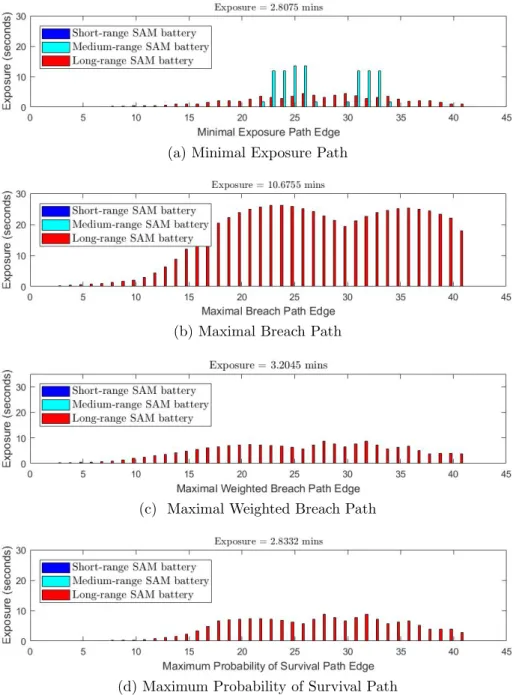
In addition to providing the defender with knowledge of potential alternative intruder path locations, analyzing the exposure values associated with each of the
alternative intrusion paths provides the defender with an assessment of the robustness of the MmEP sensor location solution. We demonstrate the MmEP solution approach and provide alternative intrusion path analysis via an air defense application example in the following section.
2.3 Testing, Results, & Analysis
We solve the mixed integer linear reformulation (16)-(24) of the bilevel Maximin Exposure Problem (3)-(10) on a 3.2 GHz PC with 6 GB of RAM, using the commercial solver IBM ILOG CPLEX 12.7. The following subsections present the chosen border security application, discuss test instance generation, and provide numerical results of the testing.
2.3.1 Illustrative Instance for Air Defense of a Border Region.
Adopting the viewpoint of a defender, we illustrate via a representative test in-stance the applicability of our MmEP formulation and solution approach to the border security application of locating ground-based assets within an Integrated Air Defense System (IADS).
Given a 600 km long by 520 km wide border region, the defender’s objective is to optimally locate two long-range (e.g., SA-21 Growler), four medium-range (e.g., SA-22 Greyhound), and six short-range (e.g., SA-24 Grinch) SAM battery assets (i.e., Bt = [2,4,6]) to maximize the ability to intercept intruding aircraft (Foss &
O’Halloran, 2014). The defender also seeks to protect three high-value assets (e.g., fielded force locations, population centers, command and control centers, etc.) located atF ={(375,420),(405,30),(450,565)}, with minimum probabilities of protection of
Cf = [0.75,0.5,0.5]. Additionally, the defender requires the long-range SAM batteries
defender’s air defense asset location solution, the intruder’s objective is to determine the least exposed intrusion path.
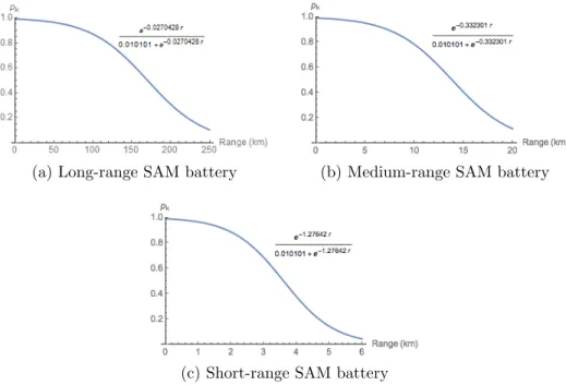
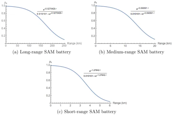
Instead of assuming binary SAM battery coverage (i.e., covered/not covered), we implement a representative probability-of-kill curve as a function of the distance from target to SAM battery, for each SAM battery type. Capabilities of these weapons for parameterizing model instances in this study are obtained from an open-source, unclassified reference (Foss & O’Halloran, 2014). The construction of the probability-of-kill curves for instances herein is notional but representative; we utilized a logit model for the probability of kill as a function of the range, assuming a probability of 0.99 for a range of zero and a probability of between 0.04 and 0.11 at the maxi-mum effective range (rmax) (Foss & O’Halloran, 2014). To artificially induce different
interceptor performance, we specified a probability of 0.55 at 65% ofrmax for the
long-range SAM batteries, a probability of 0.2 at 90% of rmax for the medium-range SAM
batteries, and a probability of 0.5 at 60% of rmax for the short-range SAM batteries.
The probability-of-kill function for each SAM battery type is depicted in Figure 2. These functions are used to calculate the exposure values for each arc resulting from the hexagonal tessellation of the border region.
In addition to the aforementioned SAM battery types, the long-range assets re-quire separate targeting and tracking radars to engage a target. However, to simplify the model, we assume that each SAM battery possesses the required radar coverage to engage enemy targets.
Furthermore, we assume for this study the defender’s incoming threat consists only of aircraft, as opposed to a wide range of threats not limited to, but including, cruise missiles and ballistic missiles. This assumption determines the coverage capabilities for each SAM battery instead of requiring the model to account for a myriad of target types. The intrusion aircraft travel at a constant velocity of 1,800 km/hr (i.e.,
(a) Long-range SAM battery (b) Medium-range SAM battery
(c) Short-range SAM battery
Figure 2. Probability-of-kill curve for each SAM battery type
|v| = 1,800 km/hr). For the baseline instance, we further assume equal exposure weights (i.e.,wt= [1,1,1]). That is, the defender does not wish to specify preferences
between SAM battery types for engaging the intruder.
2.3.2 Test Instance Generation.
Test instances for our analysis are generated by first constructing a hexagonal grid with potential sensor (i.e., SAM battery) locations positioned in the center of each hexagon. Neighboring hexagon centers are located at a defender-specified distance (in km) from each other. Herein, we adopt a distance of 30 km for initial testing in Section 2.3.3 and explore alternatives through sensitivity analyses in Section 2.3.4. The granularity of grid construction is easily adapted to suit a given situation or modeler’s needs for fidelity.
node, o, on the (w.l.o.g.) Western side of the border region to an artificial destination node, d, on the (w.l.o.g.) Eastern side of the border region, where these nodes are connected by arcs to the leftmost and rightmost hexagon arc nodes, respectively.
Unlike previous definitions of exposure in the literature which utilize the standard sensing model (1), we leverage the specific probability-of-kill functions depicted in Figure 2, as well as the target’s velocity. That is, for a type t ∈ T SAM battery located at site s ∈ S, the sensing model for a target located at the point l on arc (i, j)∈A is:
St(s, l) = pt(s, l), (47)
where pt(s, l) is the probability of kill for a target located at the Euclidean distance
from SAM battery s ∈S of type t∈T to the point l on arc (i, j)∈A.
Given a target’s location as a function of time, denoted l(τ), the cumulative exposure time of a target traversing arc (i, j) ∈ A from SAM batterys ∈ S of type
t∈T is represented as a function of either time or distance via Equation (48), wherein
τ1 and τ2 indicate the respective times at which a target starts and completes the arc
traversal, corresponding to points l1 and l2 for a given constant target velocity, |v|.
estij = Z τ2 τ1 St(s, l(τ))dτ = Z τ2 τ1 pt(s, l(τ))dτ = Z l2 l1 pt(s, l) |v| dl (48)
This exposure calculation within Equation (48) differs slightly from that used by Meguerdichian et al. (2001), wherein the author calculates cumulative exposure in-tensity vis-`a-vis cumulative exposure time, the metric of interest for the parameter
est ij.
The exposure value for each arc is calculated via numerical integration and in-cluded as a model parameter. The numerical integration requires an assumed, con-stant speed of the intruder and the probability of kill (i.e., detection) at each of a set
of discrete points along the arc. The specific probability-of-kill values at each point are determined by the probability-of-kill functions for each of the three sensor types,
t ∈T, shown in Figure 2 and the Euclidean distance between the point l and sensor locations. Therefore, we can interpret the objective function (3) as the total expected time the defender can intercept an intruder, which the defender and intruder seek to maximize and minimize, respectively.
2.3.3 Results.
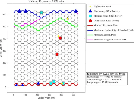
Figure 3 depicts the solution to the single-level MmEP reformulation (16)-(24) for this instance, using a 30 km spacing between potential SAM battery locations. It further depicts the four respective intruder paths, each of which is optimal for its given metric.
Figure 3. Baseline Maximin Exposure Problem solution

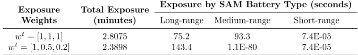
![Table 3. Exposure values for the weighted exposure (w t = [1, 0.5, 0.2]) solution](https://thumb-us.123doks.com/thumbv2/123dok_us/10217649.2925620/55.918.142.773.146.269/table-exposure-values-weighted-exposure-w-t-solution.webp)