Controlling Liu Chaotic System with Feedback Method and Its Circuit Realization

http://dx.doi.org/10.4236/ijmnta.2016.51004

Controlling Liu Chaotic System with

Feedback Method and Its Circuit Realization

Mingjun Wang

School of Information Engineering, Dalian University, Dalian, China

Received 15 October 2015; accepted 4 March 2016; published 7 March 2016

Copyright © 2016 by author and Scientific Research Publishing Inc.

This work is licensed under the Creative Commons Attribution International License (CC BY). http://creativecommons.org/licenses/by/4.0/

Abstract

In the paper, the Liu system with a feedback controller is discussed. The influence of the feedback coefficient of the controlled system is studied through Lyapunov exponents spectrum and bifurca-tion diagram. Various attractors are demonstrated not only by numerical simulabifurca-tions but also by circuit experiments. Only one feedback channel is used in our study, which is useful in communi-cation. The circuit experiments show that our study has significance in practical applications.

Keywords

Liu System, Chaotic Circuit, Chaotic Control, Circuit Realization

1. Introduction

In 1990, Ott, Grebogi and Yorke presented the OGY method to control chaos [1]. After their pioneering work, chaotic control has become a focus in nonlinear problems and a lot of work has been done in the field [2]-[4]. Nowadays, many methods have been proposed to control chaos [5] [6]. Generally speaking, there are two kinds of control ways: feedback control and nonfeedback control. Feedback methods [7]-[11] are used to stabilize the unstable periodic orbit of chaotic systems by feeding back their states. Nonfeedback methods [11]-[14] are adopted to change chaotic behaviors by applying perturbations to some parameters or variables. In the paper, we use feedback method to control the dynamic behavior of Liu system. By adjusting feedback coefficient, Liu sys-tem can be stabilized at equilibrium point or limit cycle around its equilibrium. Lyapunov exponents spectrum and bifurcation diagram are adopted to analyze the dynamic behavior of the controlled system. Numerical simu-lations and circuit experiments show the effectiveness of this method.

2. The Description of Liu System

(

)

2

x a y x

y bx kxz

z cz hx

= −

 

= −



 = − + 

  

(1)

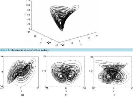
When a=10, b=40, c=2.5, h=4 and k=1, system (1) exhibits a chaotic behavior. Its attractor is shown inFigure 1. The projections of system (1)’s attractor are shown inFigure 2. System (1) has three equili-briums: S₀

(

0, 0, 0

)

, S₁

(

5, 5, 40

)

, S₂

(

− −5, 5, 40

)

.

Considering the voltage restraint of practical electronic components, let

10 , 10 , 10 .

x x

y y

z z

′ = 

 _{= ′}



 _{= ′}



(2)

Then in the new coordinate system, system (1) will be described as

(

)

2 ,

10 ,

10 .

x a y x

y bx kx z

z cz hx

′= ′− ′ 

 ′= ′− ′ ′ 

 ′= − ′+ ′ 

  

(3)

System (3) can be seemed as a reduced Liu system and the equilibriums are S₀′

(

0, 0, 0

)

, S₁′

(

0.5, 0.5 4，

)

,

(

)

2 0.5, 0.5, 4

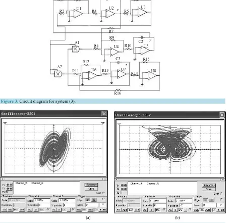
S′ − − . The circuit realization of Equation (3) is shown inFigure3.

[image:2.595.94.538.382.710.2]

InFigure 3, the voltages of C1, C2, C3 are used as variables. The relevant function can be described as

Figure 1. The chaotic attractor of Liu system.

(a) (b) (c) Figure2. The projections of Liu attractor.

120 100 80 60 40 20 0 z

y

x 40

20 0

−20

−40 −20 −10

0

10 20

−20 0 20 −30 0 30 −20 0 20

−30 0 30

0 60 120

0 60 120

3 6 3

1 4 1 5 2 4 1

9 9 6

7 10 2 5 8 10 2

2 2

12 15 12 6

2

13 14 16 3 5 11 13 3

,

,

.

R R R

x y x

R R C R R R C

R R R

y x xz

R R C R R R C

R R R R

z z x

R R R C R R R C



= −

 

 _{= −}

  

 = − +









(4)

When we choose R1 = 10 kΩ, R2 = 20 kΩ, R3 = 10 kΩ, R4 = 100 kΩ, R5 = 10 kΩ, R6 = 20 kΩ, R7 = 10 kΩ, R8

= 80 kΩ, R9 = 40 kΩ, R10 = 100 kΩ, R11 = 10 kΩ, R12 = 10 kΩ, R13 = 100 kΩ, R14 = 10 kΩ, R15 = 10 kΩ, R16 = 40

kΩ, C1 = C2 = C3 = 1 μF, the circuit system (4) is equivalent to system (3). The supplies of all active devices are

[image:3.595.242.403.88.179.2]

±18 V and the initial voltages of C1, C2, C3 are random, we obtain the experiment observations of system (4) as Figure 4(with Multisim 7.0).

Figure3. Circuit diagram for system (3).

(a) (b)

Figure4. The experiment observations of system (4). (a) x-y plane; (b) y-z plane.

R1 R3

R2 R4 R5

R6

R7

R8

R11 R12

R13

R14 R15

R16 R10 A1

A2

C2 U4

U7 _U8

C3 C1

U1 U2 _x

y U3

R9

U5

[image:3.595.90.544.269.710.2]

ComparingFigure2 andFigure4, we can know that a reduced Liu system has been realized by circuit expe-riment. Next, we will add a feedback controller to this circuit to control chaos. Various attractors will be demon-strated not only by numerical simulations but also by the circuit experiment observations.

3. Feedback Control of Liu System

Suppose we want to stabilize Liu system at equilibrium S₁ and the limit cycle surrounding S₁ respectively. For convenience, choose x as feedback variable, this feedback can be added to any of the three functions of Liu system. Applying the controller to the second function, then the controlled Liu system is described as

(

)

(

)

2

5

x a y x

y bx kxz x

z cz hx

γ

= −

 

= − − −



 _{= − +}

   

, (5)

where γ is feedback coefficient.

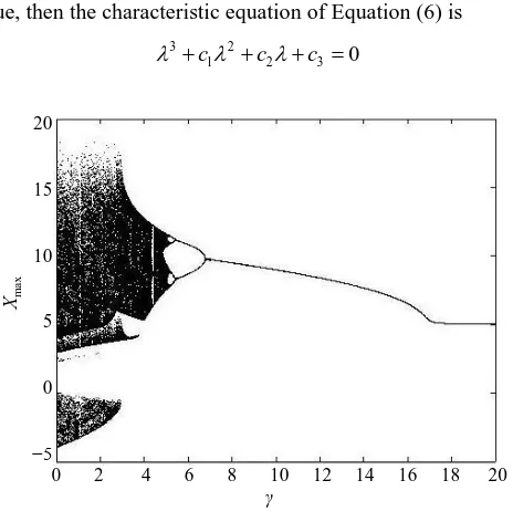
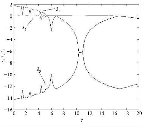
In order to study the relation between γ and system (5)’s behavior, we make the bifurcation diagram of sys-tem (5) with 0≤ ≤γ 20 inFigure5. X_max stands for the largest x in every unsteady period or steady period. When system (5) is stabilized at fixed point or system (5)’s behavior is periodic, X_max has only one value or numbered values with certain γ; When system (5)’s behavior is chaotic, X_max will have numberless values with certain γ . According to the method presented by Ramasubramanian et al. [16], we obtain the Lyapunov exponents spectrum of system (5) with 0≤ ≤γ 20 inFigure6. When the largest Lyapunov exponent λ >₁ 0, system (5)’s behavior is chaotic; When λ =₁ 0, system (5)’s behavior is periodic; When λ <₁ 0, system (5) is stabilized at fixed point. FromFigure5 andFigure6, we have the following conclusions: when γ <4.9, system (5) is chaotic (except a very narrow zone near γ =4.3, where system (5) may be periodic); when 4.9≤ <γ 16.9, system (5) is periodic; when γ ≥16.9, system (5) is stabilized at S₁.

We obtain the above conclusions by numerical calculation. In fact, the accurate range for γ to stabilize sys-tem (5) at S₁ can be obtained by theoretical calculation. Substitute the values of parameters and equilibriums, we obtain the Jacobian matrix of system (5) at S₁

(

5, 5, 40

)

:

( )

1

10 10 0

0 5 .

40 0 2.5

S

γ

−

 

 

= −_ − _

 ₋ 

 

J (6)

Suppose λ as eigenvalue, then the characteristic equation of Equation (6) is

3 2

1 2 3 0

c c c

[image:4.595.148.524.418.719.2]

λ + λ + λ+ = (7)

Figure 5.Bifurcation diagram of system (5). γ

0 2 4 6 8 10 12 14 16 18 20 20

15

10

5

0

−5

Xma

[image:4.595.197.429.474.710.2]

[image:5.595.196.429.83.291.2]

Figure 6. Lyapunov exponents spectrum of system (5).

where c₁=12.5, c₂=10γ+25, c₃=25γ +2000.

According to Routh-Hurwitz criterion, when c₁>0, c₂>0, c₃ >0 and c c_{1 2}−c₃>0, the real parts of all the eigenvalues of Equation (6) are negative, then system (5) will be stabilized at S₁

(

5, 5, 40

)

. It’s easy to ob-tain the solution γ >16.875.

4. Numerical Simulations and Circuit Realization

As for the reduced Liu system, it’s easy to obtain the relevant controlled system:

(

)

(

)

2 ,

10 0.5 ,

10 .

x a y x

y bx kxz x

z cz hx

γ = −   = − − −   = − +     (8)

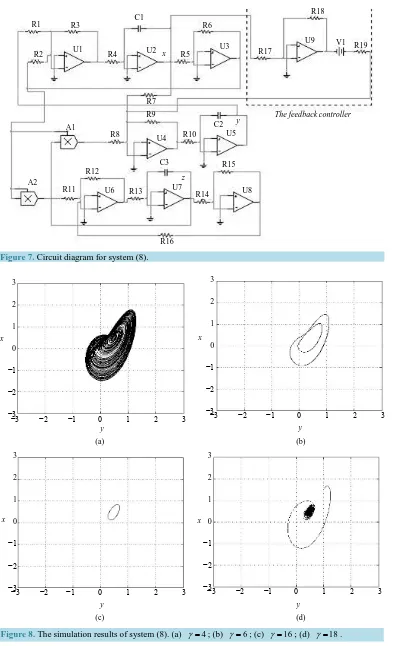
Obviously the above conclusions about γ are still available to system (8). Next we will use system (8) for numerical simulations and circuit experiments. The circuit diagram for system (8) is shown inFigure7. The re-levant function can be described as

3 6 3

1 4 1 5 2 4 1

9 9 6 9 18

1

7 10 2 5 8 10 2 19 10 2 17

2 2

12 15 12 6

2

13 14 16 3 5 11 13 3

,

,

.

R R R

x y x

R R C R R R C

R R R R R

y x xz x V

R R C R R R C R R C R

R R R R

z z x

R R R C R R R C

 = −    _{ }  = − − −         = − +     (9)

When we choose R₁₇ =R₁₈=10 kΩ, V₁=0.5 V, all other cognominal electronic components are defined as the above, then circuit system (9) is equivalent to system (8) and we can adjust R₁₉ to obtain proper feedback coefficient.

Substitute the value of R₁₇,R₁₈,R R₉, ₁₀,C V₂, ₁, we have

( )

19 400 kΩ .

R = γ (10)

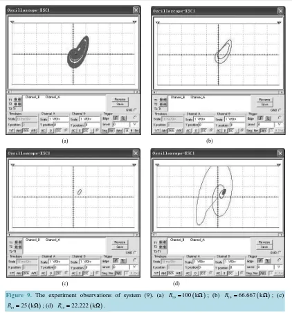
Choose typical value γ =4, 6,16,18 for numerical simulations, the simulation results of system (8) are shown inFigure8. Choose R₁₉ =100, 66.667, 25, 22.222 kΩ

( )

, we can obtain the equivalent circuit system (9), the experiment results are shown inFigure 9 (with Multisim 7.0).

2 0 −2 −4 −6 −8 −10 −12 −14 −16

Figure 7.Circuit diagram for system (8).

(a) (b)

[image:6.595.121.515.79.725.2]

(c) (d) Figure 8. The simulation results of system (8). (a) γ =4; (b) γ =6; (c) γ=16; (d) γ=18.

R1

R2

R3

R4 R5

R6

R17

R18

R19 V1 U9 U3

U2

U1 _x

y A1

R8

R7 R9

R10 U4

C2 U5

U7 z A2

R11 R12

R13 _R14

R15

R16 C3

U8 U6

The feedback controller C1

x

−3 −2 −1 0 1 2 3 y

3

2

1

0

−1

−2

−3

x

y

−3 −2 −1 0 1 2 3 3

2

1

0

−1

−2

−3

x

y

−3 −2 −1 0 1 2 3 3

2

1

0

−1

−2

−3

x

y

−3 −2 −1 0 1 2 3 3

2

1

0

−1

−2

(a) (b)

(c) (d)

Figure 9. The experiment observations of system (9). (a) R₁₉=100 kΩ

( )

; (b) R₁₉=66.667 kΩ

( )

; (c)

( )

19 25 kΩ

R = ; (d) R19=22.222 k

( )

Ω .

FromFigure 8 andFigure 9, we can know that system (8) is equivalent to system (9) in troth. When γ =4 (R₁₉ =100 kΩ), the reduced Liu system is chaotic; When γ =6 (R₁₉ =66.667 kΩ), the reduced Liu system is periodic; When γ =16 (R₁₉ =25 kΩ), the reduced Liu system’s behavior is a limit cycle around the equili-brium

(

0.5, 0.5, 4 ; When

)

γ =18 (R₁₉ =22.222 kΩ), the reduced Liu system is stabilized at

(

0.5, 0.5, 4

)

lastly. These results accord with the conclusions in Section 3.

5. Conclusion

We study the chaotic control of Liu system with feedback method in the paper. Liu chaotic system and its con-trol are realized not only by numerical simulations but also by circuit experiments. Computer simulation and circuit experiment results show the effectiveness of our method. Moreover, our control needs only one commu-nication channel, which is significant in practical applications.

Acknowledgements

[image:7.595.103.525.78.530.2]

References

[1] Ott, E., Grebogi, C. and Yorke, J.A. (1990) Controlling Chaos. Physical Review Letters, 64, 1196-1199.

http://dx.doi.org/10.1103/PhysRevLett.64.1196

[2] Chen, G. and Dong, X. (1998) From Chaos to Order: Methodologies, Perspectives and Applications. World Scientific, Singapore. http://dx.doi.org/10.1142/3033

[3] Wang, G.R., Yu, X.L. and Chen, S.G. (2001) Chaotic Control, Synchronization and Utilizing. National Defence Indus-try Press, Beijing.

[4] Guan, X.P., Fan, Z.P., Chen, C.L. and Hua, C.C. (2002) Chaotic Control and Its Application on Secure Communication. National Defence Industry Press, Beijing.

[5] Chen, G.R. and Lü, J.H. (2003) Dynamical Analyses, Control and Synchronization of the Lorenz System Family. Science Press, Beijing.

[6] Wang, X.Y. (2003) Chaos in the Complex Nonlinearity System. Electronics Industry Press, Beijing.

[7] Jang, M.J., Chen, C.L. and Chen, C.K. (2002) Sliding Mode Control of Hyperchaos in Rössler Systems. Chaos, Soli-tons & Fractals, 14, 1465-1476. http://dx.doi.org/10.1016/S0960-0779(02)00084-X

[8] Ghosh, D., Saha, P. and Chowdhury, A.R. (2010) Linear Observer Based Projective Synchronization in Delay Rössler System. Communications in Nonlinear Science and Numerical Simulation, 15, 1640-1647.

http://dx.doi.org/10.1016/j.cnsns.2009.06.019

[9] Zheng, Y.A. (2006) Controlling Chaos Using Takagi-Sugeno Fuzzy Model and Adaptive Adjustment. Chinese Physics, 15, 2549-2552. http://dx.doi.org/10.1088/1009-1963/15/11/015

[10] Gong, L.H. (2005) Study of Chaos Control Based on Adaptive Pulse Perturbation. Acta Physica Sinaca, 54, 3502- 3507.

[11] Roopaei, M., Sahraei, B.R. and Lin, T.C. (2010) Adaptive Sliding Mode Control in a Novel Class of Chaotic Systems. Communications in Nonlinear Science and Numerical Simulation, 15, 4158-4170.

http://dx.doi.org/10.1016/j.cnsns.2010.02.017

[12] Paula, A.S. and Savi, M.A. (2011) Comparative Analysis of Chaos Control Methods: A Mechanical System Case Study. International Journal of Non-Linear Mechanics, 46, 1076-1089.

http://dx.doi.org/10.1016/j.ijnonlinmec.2011.04.031

[13] Dadras, S. and Momeni, H.R. (2010) Adaptive Sliding Mode Control of Chaotic Dynamical Systems with Application to Synchronization. Mathematics and Computers in Simulation, 80, 2245-2257.

http://dx.doi.org/10.1016/j.matcom.2010.04.005

[14] Wu, Z.M., Xie, J.Y., Fang, Y.Y. and Xu, Z.Y. (2007) Controlling Chaos with Periodic Parametric Perturbations in Lo-renz System. Chaos, Solitons & Fractals, 32, 104-112. http://dx.doi.org/10.1016/j.chaos.2005.10.060

[15] Liu, C.X., Liu, T., Liu, L. and Liu, K. (2004) A New Chaotic Attractor. Chaos, Solitons & Fractals, 22, 1031-1038.

http://dx.doi.org/10.1016/j.chaos.2004.02.060