Two new approaches to spatial interpolation with inherent sidelobe suppression for imaging riometers

Two New Approaches to Spatial Interpolation with Inherent

Sidelobe Suppression for Imaging Riometers

Martin Grill, Andrew Senior, Farideh Honary

All at Department of Communication Systems, Lancaster University, UK

Abstract

Absorption images as obtained by imaging riometers such as IRIS are usually created by interpolating between absorption values for individual beams. For IRIS, the locations of the beam centres serve as grid points for subsequent linear interpolation. Although generally producing good results, the fact that the actual shape of the imaging beams is not considered, potentially introduces errors and can lead to misinterpretations.

In this paper, two alternative interpolation methods are introduced. Method A is based on measuring the similarity between simulated reception of individual point sources and actually received data. Method B uses a mathematical model of the sky brightness distribution parametrised by the received data.

All interpolation methods are applied to power data, as opposed to absorption data, in order to avoid any errors that might be introduced by intermediate processing steps, especially QDC (quiet-day curve) generation.

We apply all methods to synthetically generated test data as well as to three exemplary real datasets which are also compared to a calculated sky brightness distribution obtained from a skymap.

1 Introduction

Riometers (Relative Ionospheric Opacity Meters) have been around for decades [9]. They measure absorp-tion of cosmic background noise, caused by energetic particles ionising layers of the Earth’s ionosphere. The first riometers were widebeam riometers with a large field of view in the order of

around zenith. The search for smaller scale structures led to the development of imaging riometers which divide a similar field of view into smaller areas by forming multiple beams, usually employing phased array antennas. Cur-rent imaging riometers have between 49 beams [2] and 256 beams [13], an even higher resolution imaging riometer based on a Mills Cross beamforming technique [12] currently being under development [14].

Along with the imaging capabilities of such riometers came the necessity to spatially interpolate be-tween the measurements in order to form a real image of the observed area. Time series of these images can then be used for further studies like analysing the motion of absorption patches [10] and serve as a source for more advanced diagrams such as keograms, movies and virtual beams. These images can also be directly compared to images from other imaging instruments, for example optical cameras [5].

Currently, riometer images are usually created by interpolating between absorption values for individual beams. For IRIS, the Imaging Riometer for Ionospheric Studies [2], the locations of the beam centres serve as grid points for subsequent linear interpolation. This technique generally produces good results. However, the fact that the actual shape of the imaging beams is not considered, potentially introduces errors and can lead to misinterpretations. In particular, any given imaging beam receives signals not from one direction but from a range of directions around the beam centre, depending on the beamwidth, which itself is inversely proportional to the aperture of the receiving antenna. Also, a not always negligible fraction of signal is received from sidelobes that point in a significantly different direction from the main beam.

2 Prerequisites

In this section we introduce some general facts that are used for the observations in the following sections. We introduce the dataset that we will be using throughout this paper, highlight the role that obliquity factors play for the observations and introduce the coordinate system and the FLATM projection method that we use in this paper.

2.1 Power data, role of obliquity factors

The interpolation algorithms as discussed in this paper all deal with interpolation of power data on the positive hemisphere seen by the receiving instrument. The data is not interpreted in any way prior to processing. In particular, no assumptions are implied as to the media that the incoming signals traversed prior to reception, i.e. no correction factors (in this case known as obliquity factors) for the varying observed thickness of the absorbing layer etc. are applied to the data. In order to compare actual signals to theoretical signals based on convolution of beampatterns and skymap (see section 6), obliquity factors need to be taken into account as soon as there is an absorbing layer of electrons present. This layer appears thicker with decreasing elevation angles. See figure 1: The apparent thickness of the absorption layer decreases with

Figure 1: Obliquity factor correcting for apparent thickness of absorption layer (drawing not to scale)

observation elevation angle . The law of sines for allows us to derive angle :

!

"

#%$

'& ( # $

(1)

from which we can derive the obliquity factor ) simply by looking at*+,- (as long as/.

# $ '& ):

) "

0

1324 (2)

The left panel in figure 1 shows a plot of ) for elevation angles

,5 5 6

and&78

km (blue line). For comparison reasons, ) is also shown for an (unrealistic) height&9

0:"

km (red line). This is essentially a ‘lower amplitude’ version of ) for&;<

km. The dashed line is ) 0%=

1324 >

? )

as used in [7]. This is an approximation to equation 2 that works well for elevation angles A@CB

we plot the sky brightness distribution as derived from a skymap (see section 6). This curve was empirically found to produce good results.

Note that this use of obliquity factors is different from the traditional use where obliquity factors are applied to received power values from each beam, either ignoring the beam shape or including the effects of the beampattern in the ‘effective’ obliquity factor [7]. The obliquity factor in equation 2 does not relate to beams but simply to a certain viewing direction.

2.2 Time period

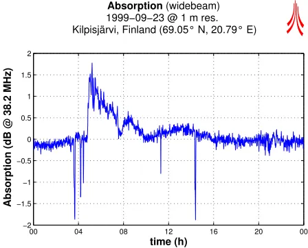
The time period chosen for the observations in this paper is 23rd September 1999. This day (as observed by the imaging riometer IRIS [2]) has quiet times, absorption events and ‘negative absorption events’ i.e. peaks in power due to interference (solar radio emissions). See figure 2 (obtained from the Multi

Absorption (widebeam) 1999−09−23 @ 1 m res. Kilpisjärvi, Finland (69.05° N, 20.79° E)

00 04 08 12 16 20 00

−2 −1.5 −1 −0.5 0 0.5 1 1.5 2

time (h)

Absorption (dB @ 38.2 MHz)

Figure 2: IRIS widebeam absorption during 1999-09-23

Instrument Analysis Toolkit MIA [11]). It is therefore an excellent dataset for comparing the performance of interpolation algorithms in various circumstances.

2.3 FLATM projection

Antenna radiation patterns and sky brightness distributions are most easily described in some sort of spher-ical coordinate system. In this paper we shall use a spherspher-ical coordinate system made up from azimuth angleD (in the XY plane, counterclockwise, starting from the positive x-axis) and elevation angle

(be-tween XY plane and direction of interest, positive denotes positive z). For visualisation purposes and further studies, this spherical dataset often needs to be mapped onto a flat two-dimensional surface. For IRIS absorption images, we commonly use a projection that we will henceforth call the ‘FLATM’ (for ‘flat metres’) projection. This is a two-stage projection that first calculates the intersection between a ray in the given direction and the ionosphere (at a given height, 90km by default) and then maps the result onto a flat surface. The whole process is shown in figure 3. This projection offers relatively little distortion around the zenith, with distortion increasing with lower elevation angles. As the surface area of the ionosphere is much greater than the area usually covered by any given instrument, the FLATM projection gives a good (i.e. relatively undistorted) representation of the signal distribution at the height of the ionosphere (or any other sphere centred on the Earth’s centre for that respect).

Figure 3: FLATM projection as used for IRIS image data. Drawn to scale. Instrument is situated at O.

3 Original IRIS interpolation algorithm

IRIS power/absorption images as created by the Multi-Instrument Analysis Toolkit (MIA) [11] use the FLATM projection to map the location of the 49 beam centres onto a flat two-dimensional grid1_{. MIA}

as-sumes that the recorded power values originate from the respective beam centre (the direction of maximum gain, also referred to as beam axis or boresight) and then uses linear interpolation to fill the space between the beam centres. An example of this can be seen in figure 4 (left panel), together with the triangles that

−1 0 1

x 105

−1.5 −1 −0.5 0 0.5 1 1.5

x 105

−1 0 1

x 105

−1.5 −1 −0.5 0 0.5 1 1.5

x 105

Figure 4: ‘Traditional’ IRIS Image Interpolation, distances are in m. Left panel shows Delaunay triangula-tion for all 49 beams, right panel shows Delaunay triangulatriangula-tion for only the ‘good’ beams.

are used internally by the two-dimensional linear interpolation algorithm. The vertices of the triangles represent the 49 beam centres. As the four corner beams (1, 7, 43, 49) have significant sidelobes [1] and the assumption of all power being concentrated at the beam centre does not even aproximately hold, these beams are usually ignored leading to an interpolated image as depicted in figure 4 (right panel). Therefore the useable working area for this algorithm is defined by the convex hull of the beam centres projected onto a flat grid by the FLATM projection, and we will overlay a white bounding box in subsequent images generated by other algorithms (which are not inherently limited to this working area) to simplify visual comparison of the results.

1_{Recent versions of MIA now use a default grid based on geographic latitude and longitude for interpolation, as geographic}

4 Method A: Correlation method

Given the radiation patterns of all beams, we can (per definition) calculate the response of each beam to a noise source in any given direction. When calculating theoretical QDCs, this is done for all directions simultaneously, yielding the total response of each beam to the given sky brightness distribution as defined by a sky map. In the correlation method, a different approach is suggested:

First, we agree on a grid of ‘directions of interest.’ This can be any arbitrary list ofE direction vectors

?

F

6GHJIDKGMLN GPO, they do not have to form a regularly spaced grid.

We then treat each direction separately: For each direction

?

F

"G we calculate the response of allQ beams

to a power source of a fixed intensity in that direction. This gives usQ received power valuesRTS , one for

each beam.

We then collectively compare this theoretical response of all beamsUNRTV:WXW+WRZY\[ to the actual recording

from these beamsU%]V%W+WXW]3Y^[ . The correlation as represented by the normalised cross correlation coefficient

1

G

0

_

Y

S4`aV R S

Y

b

S`aV

RS]cS (3)

between the two sets of values turns out to be a good estimate of how much the recording was influenced by a noise source in the particular direction in question (

?

F

"G).

We repeat these steps for each direction

?

F

"G and in doing so build up an image of the sky, represented

by the values1 G.

It is interesting to note that equation 3 resembles the equation used for finite impulse response (FIR) filters, suggesting that this algorithm can be looked upon as some sort of matched directional filtering, the

R

S being the expected responses.

4.1 Implementation note

Provided we know all potential directions of interest

?

F

"G from the outset, the theoretical beam responses R S can be calculated in advance. For any given set of input values] S we then only need to calculate the

cross-correlation coefficients1

G according to equation 3.

5 Method B: Parametrised model

We will first describe the general approach, this is not specific to using spherical harmonics, but is indeed valid for any kind of model that can be parametrised with a set number of parameters less than or equaling the number of concurrently available datapoints. We will then proceed to describe two approaches based on spherical harmonics.

5.1 (General) Curve Fitting Method

Rather than starting with an unknown power distribution (which is of course what we will be doing later on), let us assume for a moment that we know the spatial power distributiond across the visible hemisphere,

i.e.

d*>DLN ) known (4)

We also know the radiation pattern for each of the given instrument’sQ beams for all possible directions

PDeLN ):

VgfhfhfY

PDLg known (5)

Given the power distribution and the radiation patterns, we can now calculate the power response (the power received)R

Sjik

GXlnm:o for each beam

RSjikGXlHm:o qp

(

rs

it

d*PDeLN )uvSwPDeLN ) 1324

"D6 (6)

p is a constant that can be used for calibration purposes. TheQ valuesRxSjik G+lnm:o directly correspond to

the received power as measured by the receivers.

If we now find a way of representing the power distribution d in equation 4 by means ofy

5

Q

parameters instead of an infinite number of discrete values, we can work our way backwards from the actual received power values and derive (an approximation of) the original power distributiond , denoted

dzln{N|

$

o.

Let us assume thatd}l~{|

$

o is a linear combination of y functions of >DLN ), weighted by€el , i.e. a

function of the direction as specified by>DLN ) and ofy parameters€ V W+WXW€ as follows:

dal~{N| $ ouPDLg aLu€ V WXW+W€‚<€ V (ƒ V PDLg z„€… (:ƒ …PDeLN )aqW+WXW:†€ (:ƒ

/PDeLN ) (7)

In order to determine the parameters€ V WXWXW€ , we make use of equation 6, replacing the simulated

resultsR Sik G+lnm:o with the actual measurement resultsR S

0

WXW+WQ‡ from the Q beams and the ‘known’

sky brightness distributiond (equation 4) with the modelled brightness distributiond‚l~{N|

$

o (equation 7):

R S 8p ( r s it S PDLg )udzln{N| $ oNPDLg TLM€ V WXW+W€9 1324

Z"Dj (8)

We expand equation 8 using the definition of our model in equation 7:

R S ˆp

(

r s

it

S PDLg

(

I€ V (%ƒ

V >DLN )a†€… (ƒ

…"PDLg z<WXWXW%†€ (ƒ

‰PDLg )O 1324

Z"Dj (9)

Rearranging:

R S € V

( p ( r s it S PDLg ƒ

V PDLg ) 1324

D"6 (10)

€ … ( p ( r s it vSxPDLg ƒ

… PDLg ) 1324 D"6 WXWXW € ( p ( r s it

S PDeLN )

ƒ

‰>DLN ) 1Š24

"Dj

Combining all constant terms into constants1

:

RZS*

1

SjiVN€eV‹

1

Sji… € … qW+WXW%

1

Sji €  (11)

which can be written as one matrix equation for allQ beams:

dŒˆŽW (12)

In other words, we get one linear equation withy unknownsU€ V WXWXW€‡[ for each of theQ

beampat-terns. This set of equations can be solved (possibly in a least-squares sense forQ‘’y ) and therefore the

unknown model parametersU€ V WXW+W€‡[ can be determined. Once these parameters are known, the (model)

sky brightness can be calculated in any arbitrary directionPDLg by using equation 7.

5.2 Implementation employing Spherical Harmonics (B1)

Spherical harmonics [8] can be used to describe intensity distributions around a sphere. See, for example, [17] for a geophysical application. Spherical harmonics are useful because they form an orthogonal basis for functions on the sphere in a manner analogous to sines and cosines on the interval I

LN“4”)O. We are, of

Spherical harmonics are solutions to Laplace’s equation in spherical coordinates [19]. Without going into any further mathematical details, we stick to the practical description of the properties of spherical harmonics as found in [15]:

“The spherical harmonic• o–l˜—

s

it%™

L

?›š 5œž5 š

L is a function of the two coordinatesDLN on the surface

of a sphere. The spherical harmonics are orthogonal for differentš

andœ

, and they are normalised so that their integrated square over the sphere is unity.”

The degree of the spherical harmonic in question is depicted by š

, the order by œ

. The spherical harmonics are related toassociated Legendre polynomialsd

l

o by the following equation ([15]):

• o–l >DLN )ˆŸ

l o d l o 1324 D"u  GXl t (13) Since we are only dealing with a real numbers, we will use real spherical harmonics defined as follows:2

•Zo–lPDLg H¢¡ £¤’¥ “KŸ

l o 1Š24 œ )Md l o 1324 D"cL œ @ ¥ “KŸ l o ? œ )ud¦ l o 1324 D"cL œž§ Ÿ‡¨ o d,¨ o 1324 D"cL œ (14)

In both equations 13 and 14, the scaling factor K is defined as:

Ÿ l o ª© “ š 0 « ” š)?<¬ œ ¬ c­ š ¬œ ¬ c­ (15)

Note that this scaling factor (equation 15) is constant for any givenš

L

œ

. For our purposes we can therefore ignore this part, the weighting coefficients will automatically adjust themselves to accommodate for this missing factor.

For modelling the sky brightness distribution according to equation 7, we need a linear combination of a number of spherical harmonics equalling the number of available beam power readingsQ (49 in case of

the IRIS observations used in this paper). We establish a unique order between the spherical harmonics starting with

ƒ

V;®• o` ¨c¯

l `

¨

and then moving on to higher degrees, cycling through all possible orders

œ ?›š LW+WXW+L œ š

for each degree, until we arrive at

ƒ4°N± q• o`w²

¯

l `w² .

5.3 Implementation using adjusted spherical harmonics (B2)

Ordinary spherical harmonics as used in 5.2 have the disadvantage of modelling the brightness distribution over the surface of a complete sphere, resulting in relatively low-resolution at any given region of interest. Especially, in our case, a riometer will only ever ‘see’ at most a hemispherical subsection of the whole sky. It would be sensible to choose a basis which represents the power distribution over the hemisphere alone. One possibility is capped spherical harmonics [6]. However, capped spherical harmonics can be complex to implement and can result in a range of computational problems [18]. Therefore, in this paper, we use a simple approximation to spherical capped harmonics called ‘adjusted spherical harmonics’ as proposed by DeSantis [17]. It is based on a coordinate transformation that ‘adjusts’ (compresses) the elevation angles in the original definition of the spherical harmonic to those of interest (in our case the visible hemisphere). By employing these adjusted spherical harmonics, we effectively double the resolution in the hemisphere of interest. We still use the same logical order of spherical harmonics as described in section 5.2 above.

5.4 Implementation notes

As for interpolation method A (section 4), some of the values needed for evaluating equation 7 can be pre-calculated. In case of method B we do not need to know about the required directions

?

F

"G from the outset,

we only need to define a grid for numerically doing the integration in equation 10, this grid does not directly relate to the possible output directions, it is only used for the integration (summation) process, therefore limiting the accuracy of the results if chosen too wide-meshed. Once we have defined this ‘internal’ grid, theQ -by-Q matrix C (made up of the values

1

VgfhfhfYniVcfhfhfY in equation 11 can be computed. For any given set

2_{Robin Green, “Spherical Harmonic Lighting: The Gritty Details”,}

of input values] S we then only need to solve the system of linear equations (equation 11 for all

0

WXW+WQ )

and use equation 7 to calculate the interpolated power values for arbitrary directions>DLN ). Note that this

method has ‘self-interpolating’ properties, meaning that once we have calculated the coefficients1

, we are not limited to certain predefined directions. Instead, equation 7 will directly give results for all desired directions>DLN ).

6 Results

In this section, we will present the results from the two interpolation methods for three different times during 23rd September 1999 as well as for two test-cases using synthetically generated data. We will compare these results to the result obtained by the original MIA interpolation method. The results for the synthetically generated brightness distributions are compared to these very distributions. For the ‘real’ datasets, this is of course impossible since we do not know the actual sky brightness distribution in these cases. We will compare the ‘real’ datasets to the expected sky brightness distribution as derived from a skymap [4], noting that the real distribution at the time might vary greatly from this theoretical distribution, especially during active times.

In the following figures, each panel is the FLATM projection (see section 2.3) of the respective results, covering a square area ofB

« ³B

«

km. For figures containing ‘real’ data, we also show in each panel the locations of the two major radio stars [3] in this area of the sky, Cassiopeia A (white circle) and Cygnus A (white X).

6.1 Synthetic test brightness distribution 1

Figure 5: Simple testimage used as input to the interpolation algorithms. From left to right: Synthetic skymap used to synthesise power readings for all 49 IRIS beams; original MIA interpolation algorithm applied to the synthetic power readings of all IRIS beams except the four corner beams (‘good beams’); interpolation method A applied to simulated data from all 49 beams; interpolation method B1 applied to simulated data from all 49 beams; interpolation method B2 applied to simulated data from all 49 beams.

In a first step, the algorithms were compared using a synthetically generated dataset. The leftmost panel in figure 5 shows the image that was used as a skymap. Convolution of the 49 IRIS beampatterns with this skymap according to equation 6 results in 49 synthetically created ‘power readings’. The four remaining panels show the results of applying these synthetically created power readings to the different interpolation algorithms.

The original MIA interpolation algorithm produces a good representation of the input distribution. The intensity values diminish towards the outside of the interpolated area. There are low-power artefacts due to the interpolation between distant beams, especially visible at the top and bottom of the image.

Algorithm A also produces a good representation of the input distribution. However, some effect of the beam patterns is visible, and the power values trail off towards the to right and bottom left of the image.

directions. Algorithm B2 clearly shows the doubled spatial resolution compared to B1, but also seems to emphasise the problems observed with B1. There are strong overshoots in positive and negative directions and a high level of variability even inside the primary field of view.

6.2 Synthetic test brightness distribution 2

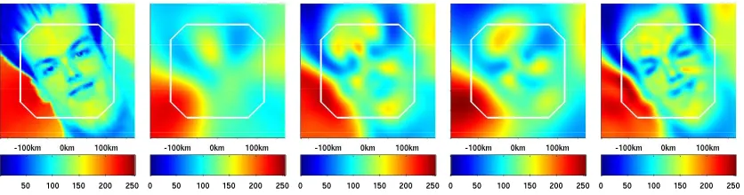
Figure 6: More detailed test image used as input to the interpolation algorithms. From left to right: Syn-thetic skymap used to synthesise power readings for all 49 IRIS beams; original MIA interpolation al-gorithm applied to the synthetic power readings of all IRIS beams except the four corner beams (‘good beams’); interpolation method A applied to simulated data from all 49 beams; interpolation method B1 applied to simulated data from all 49 beams; interpolation method B2 applied to simulated data from all 49 beams.

A more detailed input image was now used to investigate the reaction of the different algorithms to input data with higher spatial structure. See figure 6.

All algorithms seem to be able to resolve the main features (eyes, mouth). The influence of the beam-patterns is again clearly visible in the image created by algorithm A, while in the original MIA interpolated image the structure of the triangles used for the interpolation seems to show through. Both algorithms B1 and B2 seem to be doing rather well in this test case. They both emphasise the main structures rather better than the other algorithms. However, we can again observe a tendency to overshoot. Notice that both B1 and B2 tend to oscillate, especially visible for B2 as one moves from top to bottom.

6.3 Quiet Dataset

Figure 7 shows 1-minute integrated data for a quiet part of the day around 21:47UT. The skymap panel shows that we would expect to see a band of high power across the field of view. Both the traditional MIA interpolation algorithm and method A tend to break the band up into sections of varying intensity, the effects of individual imaging beams showing through. Note, however, that method A at least seems to show the continuity of this high power section to the top and to the bottom above and beyond the working area of the MIA algorithm. Opposed to this, the traditional MIA method shows areas of low power to the top and the bottom of the high power section, resulting from the linear interpolation between the outermost beam centres. This is clearly not an accurate representation of the real sky brightness. This can, of course, be eliminated by further limiting the working area of the algorithm, further reducing the field of view of the instrument.

Both methods B, whilst still showing the approximate direction of the high power band, produce several local maxima and minima within the visible area, that clearly do not resemble the actual expected brightness distribution. Notice that the two largest local maxima seem to coincide with the location of the two radio stars.

6.4 Absorption Event

Figure 8: Absorption Dataset (1999-09-23 05:23UT). From left to right: Skymap for this part of the sky at this particular moment in time; original MIA interpolation algorithm applied to actual data as received by IRIS at the time in question (only ‘good beams’ i.e. all beams except the four corner beams); interpolation method A applied to real data from all 49 beams; interpolation method B1 applied to real data from all 49 beams; interpolation method B2 applied to real data from all 49 beams.

Figure 8 is a 1-minute integrated dataset for a period of strong absorption around 05:23UT. Note the generally reduced power in all three images that are derived from real data. The image obtained by method A quite clearly shows individual beam shapes, even though those should in theory be completely removed by the algorithm. The image produced by the traditional MIA algorithm looks much smoother. It does, however, again show the sharp cutoffs, this time at the left and right, where we would expect the bright band to continue North and South. Also note the isolated brighter spot at the bottom. Looking at the skymap, we’d expect this spot to continue towards the bottom, as it indeed does for method A.

Method B, while clearly showing less overall power and the general direction of the high-power band, again seems to be the worst of the interpolation methods. It still manages to approximately show the location of the radio star. Especially method B2 shows strong oscillations in the horizontal direction.

6.5 Interference Event

Figure 9: Interference Dataset (2004-09-23 03:39UT). From left to right: Skymap for this part of the sky at this particular moment in time; original MIA interpolation algorithm applied to actual data as received by IRIS at the time in question (only ‘good beams’ i.e. all beams except the four corner beams); interpolation method A applied to real data from all 49 beams; interpolation method B1 applied to real data from all 49 beams; interpolation method B2 applied to real data from all 49 beams.

radio emission). Overall, however, the image created by method A shows strong beam artifacts, wheras the MIA image looks smooth.

Method B1 seems to show the location of the radio star, and both methods B show high intensity in the direction of the solar radio emission. As before, they fail to accurately map the overall brightness distribution, however.

7 Conclusion

We compared the traditional MIA riometer power image interpolation method to two other methods that try to take the actual antenna radiation patterns of the riometer into account. While method A seems to give good results for the 49 beam riometer IRIS, methods B1 and B2 fail to accurately reconstruct the sky brightness distribution in the general case. Some results seem to suggest that methods B1 and B2 may be useful for identifying strong but spatially small features (figure 6).

At this stage, method A seems to perform equally to the traditional MIA method, both methods leading to slightly different results due to the different underlying principles. Given that the shapes of the beampat-terns still show through in the resulting images, there seems to be no clear advantage of this method over the original MIA method. Which method is more suitable for the given task at hand will need to be decided on a case-by-case basis.

In its current form, method B fails to accurately model the brightness distribution to a high enough level of accuracy. It also suffers from oscillations and overshoots.

Although failing to deliver the increase in quality that was originally envisaged, it is hoped that this pa-per will trigger an increased interest in the area of interpolation algorithms for improving images generated by riometers, eventually leading to higher quality absorption images as a basis for high quality riometry work. The following sections gives a few ideas as to possible improvements and ongoing work.

8 Suggestions for Improvements / Future work

Research is ongoing with the aim of improving method B’s results. Currently, the matrix problem is ill-conditioned due to the inability of the IRIS beam pattern to discriminate between a large number of configurations of the model power distribution, effectively resulting in fewer equations than unknowns. In section 5.1, it has already been hinted at the fact that the number of equations used to model the brightness distribution (y ) does not have to equal the number available data points (Q ). In fact, havingy

§

Q

allows for least-square fits and also for error ranges to be included in the approximation. This has the potential to significantly increase the quality of method B’s output, along with a built-in quality indicator. Along the same lines, it is possible to add additional spatial contraints to increase the number of available equations. This will lead to a better conditioning of the matrix problem.

It may also be possible to improve method B’s results by choosing different interpolation functions for the curve fitting process.

Finally, it has to be noted that interpolation of power images is only the first step to deriving absorption data in arbitrary (virtual beam) directions. Based on the interpolation algorithms presented in this paper, quiet day curves (QDCs) can potentially be calculated for arbitrary directions, enabling the derivation of absorption in these directions and therefore the creation of absorption images on arbitrary grids and with arbitrary resolutions.

Appendix A: Image interpolation with Spherical Harmonics

To confirm the spatial resolution that image approximation using spherical harmonics is able to produce, three test images have been approximated by calculating the first 49 and 256 coefficients for both the standard spherical harmonics approach (section 5.2) and the adjusted spherical harmonics approach (see section 5.3), see the figures 10, 11 and 12. Clearly, spherical harmonics are able to reproduce the source image with sufficient details, but deriving the coefficients from real-world data is non-trivial.

References

[1] Noach Amitay, Victor Galindo, and Chen Pang Wu. Theory and analysis of phased array antennas. Wiley-Interscience, New York, 1972.

[2] S. Browne, J. K. Hargreaves, and B. Honary. An imaging riometer for ionospheric studies.Electronics

and Communication Engineering Journal, 7(5):209–217, October 1995.

[3] Bernhard F. Burke and Francis Graham-Smith. An Introduction to Radio Astronomy. Cambridge University Press, 1st edition, 1997.

[4] H. V. Cane. A 30 MHz map of the whole sky.Australian Journal of Physics, 31:561–565, 1978. [5] C. F. del Pozo, M. J. Kosch, and F. Honary. Estimation of the characteristic energy of electron

precipitation.Annales Geophysicae — Atmospheres, Hydrospheres and Space Sciences, 20(9):1349– 1359, 2002.

[6] G. V. Haines. Spherical cap harmonic analysis. Journal of Geophysical Research, 90:2583–2591, 1985.

[7] J. K. Hargreaves and D. L. Detrick. Application of polar cap absorption events to the calibration of riometer systems. Radio Science, 37(3):7/1–7/11, 2002.

[8] Ernest William Hobson.The theory of spherical and ellipsoidal harmonics. 1955.

[9] C. G. Little and H. Leinbach. The riometer - a device for continuous measurement of ionospheric absorption.Proceedings of the Institution of Radio Engineers, 47:315–320, 1959.

[10] R. A. Makarevitch, F. Honary, I. W. McCrea, and V. S. C. Howells. Imaging riometer observations of drifting absorption patches in the morning sector. Annales Geophysicae — Atmospheres,

Figure 10: Interpolating an image using spherical harmonics. From left to right: original image; interpo-lated image using 49 coefficients and standard spherical harmonics; interpointerpo-lated image using 256 coeffi-cients and standard spherical harmonics; interpolated image using 49 coefficoeffi-cients and adjusted spherical harmonics; interpolated image using 256 coefficients and adjusted spherical harmonics.

Figure 11: Interpolating an image using spherical harmonics. Panels as in figure 10.

[11] S. R. Marple and F. Honary. A multi-instrument data analysis toolbox. Advances in Polar Upper

Atmosphere Research, 18:120–130, September 2004.

[12] B. Y. Mills and A. G. Little. A high-resolution aerial system of a new type. Australian Journal of Physics, 6:272–278, 1953.

[13] Yasuhiro Murayama, Hirotaka Mori, Shoji Kainuma, Mamoru Ishi, Ichizo Nishimuta, Kiyoshi Igarashi, Hisao Yamagishi, and Masanori Nishino. Development of a high-resolution imaging ri-ometer for the middle and upper atmosphere observation program at Poker Flat, Alaska. Journal of Atmospheric and Solar-Terrestrial Physics, 59(8):925–937, 1997.

[14] E. Nielsen and T. Hagfors. Plans for a new rio-imager experiment in Northern Scandinavia. Journal of Atmospheric and Solar-Terrestrial Physics, 59(8):939–949, 1997.

[15] William H. Press, Brian P. Flannery, Saul A. Teukolsky, and William T. Vettering.Numerical Recipes in C. Cambridge University Press, 1st edition, 1988.

[16] T. J. Rosenberg, D. L. Detrick, D. Venkatesan, and G. van Bavel. A comparitive study of imaging and broad-beam riometer measurements: The effect of spatial strucure on the frequency dependence of auroral absorption. Journal of Geophysical Research — Space Physics, 96(A10):17793–17803, October 1991.

[17] A. De Santis. Conventional spherical harmonic analysis for regional modelling of the geomagnetic field. Geophysical Research Letters, 19:1065–1067, 1992.

[18] A. De Santis and J.M. Torta. Spherical cap harmonic analysis: a comment on its proper use for local gravity field representation.Journal of Geodesy, 71:526–532, 1997.