H Infinite Controller Design of Singular Networked Control Systems

(1)

Published Online February 2014 (http://www.scirp.org/journal/ica) http://dx.doi.org/10.4236/ica.2014.51004

H-Infinite Controller Design of Singular Networked

Control Systems

Zhanzhi Qiu, Lei Shi

Software Technology Institute, Dalian Jiaotong University, Dalian, China Email: [email protected], [email protected]

Received December 5, 2013; revised January 5, 2014; accepted January 12, 2014

Copyright © 2014 Zhanzhi Qiu, Lei Shi. This is an open access article distributed under the Creative Commons Attribution License, which permits unrestricted use, distribution, and reproduction in any medium, provided the original work is properly cited. In accor- dance of the Creative Commons Attribution License all Copyrights © 2014 are reserved for SCIRP and the owner of the intellectual property Zhanzhi Qiu, Lei Shi. All Copyright © 2014 are guarded by law and by SCIRP as a guardian.

ABSTRACT

This paper investigates the H_∞ controller design method for a class of singular networked control systems (SNCS) based on the singular plant. In view of the network-induced delay less than or equal to a sampling period, finite external disturbance, clock-driven sensors, event-driven controller and actuators as well as impulse behavior and structural instability of singular plants, the H_∞ controller design method of SNCS with state feed- back way and dynamic output feedback way is investigated respectively by means of the linear matrix inequality method. The existence condition of H∞ control law, the solving approaches of H∞ controller parameters and

disturbance attenuation degree are presented. Finally, a simulation example is given to illustrate the effectiveness and feasibility of the presented method.

KEYWORDS

Singular Networked Control Systems; H∞ Controller Design; Network-Induced Delay;

Disturbance Attenuation Degree

1. Introduction

Networked control system (NCS) is a distributed real- time feedback control system where the system node situates different geographical position exchange data and control signal with controller via communication network [1]. Due to limited network bandwidth and restraint of communication mechanism, unexpected phenomenon such as networked-induced delay and data packet loss exist typically in communication channel, which often makes NCS lose invariability, integrality, causality and certainty [2], therefore, the study of NCS is more com- plicated and challenging. The traditional control theories and methods built on point-to point direct control system are not suitable for NCS, which makes rapid develop- ment on NCS over the past few years. Since the end of last century, the research of NCS experiences the process of from simple to complex, from single to comprehensive and from special to general. A large number of results have been reported, for instance, system complexity analysis [3,4], quantized dynamic output feedback control

[5], observer-based controller design [6], state estimation and stabilization [7], H_∞ control method [8,9], fault- tolerant control [10], guaranteed cost control [11], co- design [12], etc.

It should be pointed out that, most of the results in the existing literature are focused on linear normal system, while the study of singular networked control system (SNCS) based on singular system has not been addressed intensively. Since the dynamics of singular system is quite different from normal linear/nonlinear system, and has many characteristics such as pulse characteristics, no causality, no solution, no uniqueness, structure instability, etc. [13]. Therefore, the investigation of SNCS is rather interesting. In fact, the research about SNCS is still in the primary stage. The existing results are limited to system modeling, stability analysis and ordinary control method [14-18].

(2)

25

and NCS. In this work, network-induced delay, limited input disturbance, impulse behaviour are taken into si- multaneous consideration. The H∞ control method of

SNCS with state feedback way and dynamic output feedback way is investigated respectively by means of the linear matrix inequality method. The existence condition of H∞ control law, the solving approaches of

H∞ controller parameters and disturbance attenuation

degree in different feedback way are presented. Finally, a simulation example is given to illustrate the effectiveness and feasibility of the proposed method.

2. Problem Formulation

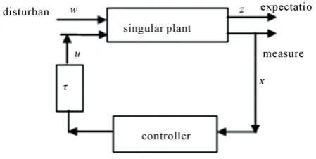
The SNCS based on singular plant is shownin Figure 1. where

u x y w

, , ,

and z_{are control input, measure state}

or measure output, external disturbance andexpectation output respectively. The plant is a class of singular plant, and the data packets are transmitted via network. Choice of communication network and determine of feedback control way depend on site state and control goals of plant. The aim are to guarantee systems stable, for external disturbance, expected output of the system is not affected as far as possibleor very small.

In this paper, it is assumed that sensors are driven by clock, controller and actuators are driven by event, the measuresensorssample the state value or output value of the plant with period

T

, the measured value are transmitted to the remote controller via network after A/D conversion and packaging; controller respond immediately to calculate control law and transmit to actuator node after receiving the information from sensors, and actuator node work immediately to implementadjustment job after receiving the control signal from the controller.

[image:2.595.310.535.86.199.2]

As the system is shown in Figure 1, there are two kinds of problem to consider: the singular characteristics the plant and the network communication characteristics of the control network. For singular plant, its state response contains not only the exponential term similar to normal systems, but also the pulse term and input derivative item, which will make the whole system have pulse behavior. The pulse reduces not only the performance and even leads to unstable system, which is a fatal destructiveness for the system. For network communication,as a result oflimited network bandwidth and restraint of communication mechanism, the network communication obtains uncertainty and complexity. The most prominent problem is network-induced delay. As seen in Figure 1, τ_sc denotes the network-induced delay between sensor node and controller node, and τ_ca denotes the network-induced delay between controller node and actuator node, and all of the network-induced delay of closed-loop system τ τ= _sc+τ_ca. The delay performance depends on the communication protocol

Figure 1. General structure of SNCS.

employed by the communication network. The delay maybe is constant, random, limited, even Markov chain feature. In order to enhance the system performance, in a general way, we make as far as possible it constant. Furthermore, there exists single packet and multiple packet transmission, data packet loss, network connec- tion interrupt and channel interference etc. All of these problems will make the structure characteristics of close- loop systems change, and influence the stability and control performance of the SNCS.

In this paper, the considered singular plant is shown in Equation (1):

( )

(

)

( )

0

1 1

2 2

Ex t Ax t Bu t H w t

y t C x t H w t

z t C x t H w t

τ

= + − +

 

= +



 ₌ ₊





(1)

wherex t

( )

∈Rn, u t

( )

∈Rm, y t

( )

∈Rl and z t

( )

∈Rl are state vector, control input vector, output vector and expectation output vector, respectively. E A, ∈Rn m× ,

n m

B∈R× _and l n

C∈R× _{are constant matrix,}

E

is singular matrix, i.e. rank E

( )

=qn; w t

( )

is finite

external disturbance, H H H₀, ₁, ₂ are corresponding dimension constant matrix.

Throughout this paper, the following assumptions are made:

1) The singular plant is regular and impulse free, which is achieved by adjustingthe part structure and com- ponentconfiguration of plant, such that one of the following holds:

a) deg det

(

sE−A

)

=rank

( )

E

b) rank E 0 n rank

( )

E

A E

 _{= +}

 

 

2) The network-induced delay of closed-loop system is less than or equal to a sampling period, i.e.

τ ≤

T

, and the sample period

T

is constant, which is achieved bychoosing suitable communication protocol of control network and designing part device of the system.

(3)

4) The external input disturbance of the plant is finite energy, i.e. the close-loop transfer function from w k

( )

to z k

( )

satisfies

T z

( )



β

,

β

is a scalar.

According to condition (1), when the singular plant is regular and impulse free, there are always two nonsingular matrices P Q,, such that

1 0 0 , 0 0 0 r n r A I PEQ PAQ I ₋     =_ _ _{= } _         , 1 1 0 2 2 , W B PH PB W B     =_ _ =_{ }       ,

[

]

[

]

1 11 12 , 2 21 22 .

C Q= C C C Q = C C

Let

( )

1 1

2 x t Q x t

x t

− _{= } 



 

 , Equation (1) can be equiva-

lent transformed as:

( )

(

)

( )

(

)

( )

1 1 1 1 1

2 2 2

11 1 12 2 1

21 1 22 2 2

0

x t A x t B u t W w t

x t B u t W w t

y t C x t C x t H w t

z t C x t C x t H w t

τ τ = + − +   = + − +   = + +   ₌ ₊ ₊   (2)

When the network-induced delay

τ

≤T, control input

u

_{is piecewise continuous in a sampling period, the dis-}

crete-time model of Equation (2) in a sampling period can be shown as Equation (3):

(

)

( )

( ) (

)

( ) ( )

( )

(

)

( )

1 1 11

10 0

2 2 2

11 1 12 2 1

21 1 22 2 2

1 1

1

d

x k A x k B u k

B u k W w k

x k B u k W w k

y k C x k C x k H w k

z k C x k C x k H w k

τ τ + = + −   + +   _{= −} _{− −}   ₌ ₊ ₊   ₌ ₊ ₊  (3) where 1 eA T

d

A = ,

( )

1

10 ₀ e 1d

T _{A t}

B τ =

∫

−τ B t,

( )

1

11 e 1d

T _{A t} T

B τ =

∫

₋_τ B t

,

1

0 ₀ e 1d

T _{A t}

W =

∫

W t

.

The state feedback controller model is shown in Equa- tion (4).

( )

[

]

1

( )

_{( )}

1 2

2 x k

u k K K

x k

 

= _ _

  (4)

Combine Equation (3) with Equation (4), the following closed-loop system is obtained

(

)

(

( )

)

( )

(

)

(

)

( )

(

)

( )

(

)

( )

(

) (

) ( )

1 10 1 1

11 10 2 2

0 10 2 2

1 1 2 2 2 2

21 1 22 2 2 22 2

1

d

x k A B K x k

B B K B u k

W B K W w k

u k K x k K B u k K W w k

z k C x k C B u k H C W w k

τ τ τ τ  + = +   + − −  ₊ ₋   = − − −   ₌ ₋ _{− +} ₋ 

Let augmented state vector T

( )

T

(

)

T

1

ˆ 1

x=_x k u k− _ ,

therefore, the close-loop model of state feedback SNCS is as follows:

(

)

(

( )

)

(

( )

)

( )

_{( )}

10 1 11 10 2 2

1 2 2

0 10 2 2

2

ˆ 1 Ad B K B B K B ˆ

x k x

K K B

W B K W

w k K W

τ τ τ

τ  + −  + =   −     −   +  ₋    (5) When the state variables are not measurable, or partial state is measurable, we will put to use the following dynamic output feedback controller:

(

)

( )

1

c c c c

c c

x k A x k B y k

u k C x k

+ = +



 ₌



(6)

Combine Equation (3) and Equation (6), the following can be obtained:

(

)

( )

( ) (

)

( )

(

)

( )

(

) (

) ( )

( )

(

)

(

) ( )

1 1 10

11 0

11 1 12

2 1 12 2

21 1 22 2

2 22 2

1

d c c

c c c c c

c c

x k A x k B C x k

B u k W w k

x k B C x k A x k B C

B u k B H B C W w k

u k C x k

z k C x k C B u k

H C W w k

τ τ + = +   + − +   _{+ =} ₊ ₋   _× _{− +} ₋   ₌   ₌ ₋ ₋   + − 

Let augmented state vector

( )

(

)

T

T T T

1 c 1

x=_x k x k u k− _ , then, the close-loop

model of dynamic output feedback SNCS is shown in Equation (7):

(

)

( )

10 11

11 12 2

0

1 12 2

1

0 0

0

d c

c c c

c

c c

A B C B

x k B C A B C B x k

C

W

B H B C W w k

τ τ     + =_ − _         +_ − _     (7)

(4)

27

of SNCS is a linear time-invariant system, when τ changes with time, the close-loop system model of SNCS is a time-varyingsystem.

3. H

∞

Controller Design

Define 1: Given a positive constant

γ

, for the state feedback case, if close-loop system (5) is asymptotically stable under zero initial condition

(

x

( )

0 =

0 )

,external disturbance w k

( )

and expected output z k

( )

satisfy

H∞ norm constraint condition z k

( )

₂ ≤

γ

w k

( )

₂, then,

singular plant (1) realizes

γ −

second best state feedback H∞ control, the system disturbance attenuation

degree is defined as

γ

, the corresponding state control law is defined as

γ −

second best state feedback H∞

control law; further optimization make γ minimum, in this case, the state feedback H∞control law is defined as

γ −

best state feedback H∞ control law.

Define 2: Given a positive constant

γ

, for the dynamic output feedback case, if close-loop system (7) is asymptotically stable, and when zero initial state

( )

(

x

0 =

0 )

, external disturbance w k

( )

and expectation output z k

( )

satisfy H_∞ norm constraint condition

( )

₂

( )

₂

z k

≤

γ

w k

, then singular plant (1) realizes

γ −

second best dynamic output feedback H∞ control, the

system disturbance attenuation degrees is defined as

γ

, the corresponding dynamic output feedback control law is defined as

γ

− second best dynamic output feedback

H∞ control law; further optimization make

γ

mini-mum, in this case, the dynamic output feedback H∞

control law is defined as

γ −

best dynamic output feed-back H∞ control law.

Lemma1: [19] For real matrices W M N, , and F k

( )

,

where

W

is symmetric, F k

( )

satisfies FT

( ) ( )

k F k ≤I, then below matrix inequality

( )

T T

( )

T

0,

W+MF k N+N F k M <

if and only if there is a scale

ε

>

0

, such that

T 1 T

0.

W+εMM +ε−N N <

3.1. State Feedback

H_∞

Controller Design

Theorem 1: Without regard to the external disturbance, under the control of state feedback controller (4), if there exist positive definite matricesS,R, such that

T T

1 1

T T

2 3

1 2

1 3

0 0

0 0 0

S SM SK

R RM RM

M S M R S

K S M R R

− 

 ₋ 

 _{ <}

 ₋ 

 

−

 

 

(8)

where

( )

1 d 10 1

M =A +B τ K ,

( )

2 11 10 2 2

M =B τ −B τ K B ,

3 2 2 M = −K B ,

then state feedback SNCS (5) is asymptotically stable. Proof: Choose positive definite matrices

S

_and R, define a Lyapunov function as follows:

( )

T

( ) ( )

T

(

) (

)

1 1 1 1

V k =x k Sx k +u k− Ru k− .

then the forward differential of V k

( )

along trajectory of closed-loop system (5) is as follows:

( )

(

) (

)

( ) ( )

(

) (

)

( )

T T

1 1

T T

1 1

T

1 1

ˆ ˆ

V k x k Sx k u k Ru k

x k Sx k u k Ru k

x k x k

∆ = + + +

− − − −

=

∏

where

( )

T

( )

T

(

)

T

1

ˆ 1

x k =_x k u k− _ ,

T T T T

1 1 1 1 1 2 1 3

T T T T

2 1 3 1 2 2 3 3

M SM K RK S M SM K RM

M SM M RK M SM M RM R

 + − + 

Π =  ₊ ₊ ₋ 

 

By Lyapunov stability theory, if ∆V K

( )

<0,then system (5) is asymptotically stable, so,the asymptotically stability condition is as follows:

T T T T

1 1 1 1 1 2 1 3

T T T T

2 1 3 1 2 2 3 3

0

M SM K RK S M SM K RM

M SM M RK K SM M RM R

 + − + 

<

 

+ + −

  (9)

By Schur complement, Equation (9) can be transformed as:

T T

1 1

T T

2 3

1 1 2

1

1 3

0 0

0 0 0

S M K

R M M

M M S

K M R

− −

− 

 ₋ 

 _{ <}

 ₋ 

 

−

 

 

(10)

Multiplying

diag

(

S

−1

,

R

−1

, ,

I I

)

on the left side and the right side of equation (10), it is derived that

1 1 T 1 T

1 1

1 1 T 1 T

2 3

1 1 1

1 2

1 1 1

1 3

0 0

0 0 0

S S M S K

R R M R M

M S M R S

K S M R R

− − −

 − 

 

−

 _{ <}

 ₋ 

 

−

 

 

(11)

Let S =S−1,R=R−1, then Equation (11) is equivalent to Equation (8), the proof is completed.

(5)

T T T

1 1 21

T T T

2 3 4

2 T T T

3 4 5

1

1 2 3

1

1 3 4

21 4 5

0 0

0

0 0

S M K C

R M M M

I W W W

M M W S

K M W R

C M W I

γ

− −

− 

 ₋ 

 

 ₋ 

<

 

−

 

 ₋ 

 

−

 

 

(12)

where

4 22 2, 5 2 22 2 M = −C B W =H −C W ,

4 2 2 W = −K W ,

( )

3 0 10 2 2

W =W −B τ K W ,

then singular plant (1) canrealize

γ −

second best state feedback H∞ control.

Proof: The external disturbance is taken into account,

according to definition 1, to make

( )

2 2

z k ≤

γ

w k

hold, Let T

( ) ( )

2 T

( ) ( )

0 z

k

J z k z k γ w k w k

∞ =

 

=

∑

_ − _, choo-

sepositive definite matrices S R, , and define a Lyapu- novfunction V k

( )

=x₁T

( ) ( )

k Sx k₁ +uT

(

k−1

) (

Ru k−1

)

. For close-loop system (5), when meet theorem 1, the system is asymptotically stable, in the zero initial conditions, for∀w k

( )

∈L₂

[

0,∞

)

, it is derived as

( ) ( )

T

( ) ( )

( )

T 2 '

0

k

z k z k γ w k w k V k

∞ =

 ₋ _{+ ∆} _<

 

∑

( ) ( )

T

( ) ( )

( )

T 2 ' T

0 z

k z k

−

γ

w

k w k

+ ∆

V k

= Φ <

x

 

x

where T

( )

T

(

)

T

( )

T

1 1

x=_x k u k− w k _ ,

11

21 22

31 32 33

* *

* 0

A

A A

A A A

 

 

Φ =_ _<

 

 

(13)

T T T

11 1 1 1 1 21 21

A =M SM +K RK − +S C C _, T T T

21 2 1 3 1 4 21

A =M SM +M RK +M C

T T T

22 2 2 3 3 4 4

A =M SM +M RM − +R M M _, T T T

31 3 1 4 1 5 21

A =W SM +W RK +W C

T T T

32 3 2 4 3 5 4

A =W SM +W RM +W M _, T T T 2

33 3 3 5 5 4 4

A =W SW +W W +W RW −γ I

By Schur complement, Equation (13) can be transformed as

T T T T T

21 21 21 4 21 5 1 1

T T T T T

4 21 4 4 4 5 2 3

T T T 2 T T

5 21 5 4 5 5 3 4

1

1 2 3

1

1 3 4

0 0 0

S C C C M C W M K

M C R M M M W M M

W C W M W W I W W

M M W S

K M W R

γ

− −

− + 

 _{− +} 

 

 −  <

 

−

 

 ₋ 

 

(14)

Similarly, further transform, Equation (12) can be derived, the proof is completed.

Theorem 3: For singular plant (1), under the control of state feedback controller (4), if there exist symmetric

positive definite matrices ˆ ˆS R, , matrices Y Y Y₁, ₂, ₃, scalars ε>0,ε₁>0,β >0 and compatible dimension unit matrixI, such that

d 10 1 11 0

1

21 22 2 2 22 2

2 2

2 2 1

T 3 10

2 1

ˆ

ˆ 0

0 0

ˆ ˆ ˆ

ˆ

0 0 0

ˆ ˆ ₀ ₀

ˆ

0 0 0 0

ˆ

0 0 0 0 0

0 0 0 0 0 0 0

0 0 0 0 0 0 0 0

S

R

I

A S B Y B R W S

Y R

C S C B R H C W I

B R W I

Y B I

Y I

β

ε ε

 − ∗ ∗ ∗ ∗ ∗ ∗ ∗ ∗ ∗ 

 

− ∗ ∗ ∗ ∗ ∗ ∗ ∗ ∗

 

 ₋ _∗ _∗ _∗ _∗ _∗ _∗ _∗ 

 

 ₊ ₋ _∗ _∗ _∗ _∗ _∗ _∗ 

 

 − ∗ ∗ ∗ ∗ ∗ 

 

− − − ∗ ∗ ∗ ∗

 

− ∗ ∗ ∗

 

 ₋ _∗ _∗ 

 

 − ∗

 ₋

 

0

<

 

(6)

29

then the disturbance attenuation degree γ = β ,

γ −

second best state feedback H∞ controller is as following:

( )

1 T 1

( )

_{( )}

1 2 1

2

ˆ x k

u k Y S Y

x k

ε

−  

 

=_ _ _

   (16)

Proof: For singular plant (1), if

γ −

second best state feedback H∞ control law exists, then theorem 2 is true.

Spread out M₁~M W₄, ₃~W₅, then Equation (12) can be expressed as

2

1 d 10 1 11 10 2 2 0 10 2 2

1

1 2 2 2 2

21 22 2 2 22 2

0

0 0

0

0 0

S

R

I

A B K B B K B W B K W S

K K B K W R

C C B H C W I

γ

− −

− ∗ ∗ ∗ ∗ ∗

 

 ₋ _∗ _∗ _∗ _∗

 

 − ∗ ∗ ∗

<

 ₊ ₋ ₋ ₋ _∗ _∗

 

 ₋ ₋ ₋ _∗

 

− − −

 

 

(17)

Equation (17) can be written as:

[

]

T

2

T 2 2

1

d 10 1 11 0 10 2 10 2

1

1 2 2 2 2

21 22 2 2 22 2

0 0

0 * 0 0

0 0 0 0

0 0 0 0 0

0 0 0

0 0 0 0

S

R

I

I B W I

A B K B W S B K B K

K K B K W R

C C B H C W I

γ

− −

− ∗ ∗ ∗ ∗ ∗

     

 ₋ _∗ _∗ _∗ _∗     

     

 − ∗ ∗ ∗     

+ <

 ₊ ₋ _∗ _∗  ₋  ₋ 

     

 ₋ ₋ ₋ _∗     

     

− − −    

 _{ } _ _ _

 

(18)

From lemma 1 and Schur complement, Equation (18) can be transformed as

T 2

2 T

2

d 10 1 11 0

1

1 2 2 2 2

21 22 2 2 22 2

2 2

0 0

0 0 0

0 0 0 0

S

R B

I W

A B K B W

K K B K W R

C C B H C W I

B W I

γ

ε

−

− ∗ ∗ ∗ ∗ ∗

 

 ₋ _∗ _∗ _∗ _∗ 

 

 − ∗ ∗ ∗ 

 

<

+ Γ ∗ ∗

 

 ₋ ₋ ₋ _∗ 

 

− − −

 

 ₋ 

 

(19)

where Γ = −S−1+

ε

B K₁₀ ₂

(

B K₁₀ ₂

)

T. further transform, Equation (19) is derived that

2

1

d 10 1 11 0

1 1

21 22 2 2 22 2

2 2

2 2 1

T 10 2

T

1 2 1

0

0 0

0 0 0

0

0 0

0 0 0 0

0 0 0 0 0

0 0 0 ( ) 0 0 0 0

0 0 0 0 0 0 0 0

S

R

I

A B K B W S

K R

C C B H C W I

B W I

B K I

K I

γ

ε ε

−

− ∗ ∗ ∗ ∗ ∗ ∗ ∗ ∗ ∗

 

 ₋ _∗ _∗ _∗ _∗ _∗ _∗ _∗ _∗ 

 

 − ∗ ∗ ∗ ∗ ∗ ∗ ∗ 

 

+ − ∗ ∗ ∗ ∗ ∗ ∗

 

 ₋ _∗ _∗ _∗ _∗ _∗ 

  <

− − − ∗ ∗ ∗ ∗

 

 ₋ _∗ _∗ _∗ 

 

− ∗ ∗

 

 ₋ _∗ 

 

 − 

 

(20)

Multiplying

diag

(

S

−1

,

R

−1

, , , , , , , ,

I I I I I I I I

)

on the left side and the right side of Equation (20), and Let

1 1

ˆ _,ˆ

S=S− R=R− , and then Letβ γ₌ 2_,

1 1ˆ

Y =K S,

T

2 1 2

Y =εK , T

3 2

(7)

Theorem 4: For singular plant (1), if the following optimization problem has feasible solutions:

1

min

0, 0, 0

s.t. (15)

β

ε> ε > β > (21)

the minimum disturbance attenuation degree is

γ

∗=

β

∗,

γ −

best state feedback H∞ controller is

( )

1 T 1

( )

_{( )}

1 2 1

2

ˆ x k

u k Y S Y

x k

ε

∗ ₌_ ∗ ∗− ∗ ∗_ 

 

 _{ } _ (22)

By means of feasibility problem Solver “feasp” and optimization problem Solver “mincx” of MATLAB LMI tool-box, if the feasible solutions of theorem 3 and theorem 4 exist,

γ −

second best state feedback H∞ control-

ler,

γ −

best state feedback H∞ controller as well as cor-

responding disturbance attenuation degree are obtained.

3.2. Dynamic Output Feedback

H_∞

Controller Design

Theorem 5: when the external disturbance is not taken into account, under the control of dynamic output feedback controller, if there exist positive definite matrices

, ,

P Q S  , such that

5 6

7 8

0

0 0

0

0 0 0 0

d

c

c P

Q S

A P M Q M S P

M P A Q M S Q

C Q S

 − ∗ ∗ ∗ ∗ ∗ 

 

− ∗ ∗ ∗ ∗

 

 ₋ _∗ _∗ _∗ 

<

 

− ∗ ∗

 

 ₋ _∗ 

 

−

 

 

 



 

  



 

(23)

w h e r e M₅=B₁₀

( )

τ C_c , M₆=B₁₁

( )

τ , M₇=B C_c ₁₁,

8 c 12 2

M = −B C B , then dynamic output feedback SNCS (7) is asymptotically stable.

Proof: Let M₅=B₁₀

( )

τ C_c,M₆ =B₁₁

( )

τ ,M₇=B C_c ₁₁,

8 c 12 2

M = −B C B ,W₆ =B_c

(

H₁−C W₁₂ ₂

)

, then Equation(7) can be written as

(

1

)

7 5 68

( )

06

( )

0 0 0

d c c

A M M W

x k M A M x k W w k

C

   

   

+ =_ _ +_{ }

   _{ }

 

When the external disturbance of system is not taken into account, choose positive definite matrices P Q S, ,

and define a Lyapunov as follows:

( )

( ) ( )

( )

(

) (

)

1 1

T T

c c T

V k x k Px k x k Qx k

u k Su k

= +

+ − −

Then the forward differential of V k

( )

along trajectory of close-loop system (7) is as follows:

( )

T

V k x x

∆ = Ψ 

where

( )

T

( )

T

( )

T

(

)

T

1 c 1

x k =_x k x k u k− _ ,

11

21 22

31 32 33

D

D D

D D D

∗ ∗

 

 

Ψ =_ ∗ _

 

 

11 7 7

T T

d d

D = A PA +M QM −P_, T T

21 5 d c 7

D =M PA +A QM

T T

22 5 5

T

c c c c

D =M PM +A QA +C SC −Q

T T

31 6 d 8 7

D =M PA +M QM _, T T

32 6 5 8 c

D =M PM +M QA

T T

33 6 6 8 8

D =M PM +M QM −S

By Lyapunov stability theory, the asymptotically stability condition of system (7) is as follows:

11

21 22

31 32 33

0

D

D D

D D D

∗ ∗

 

 _{∗ <}

 

 

(24)

By Schur complement, the above Equation (24) can be transformed as:

1 5 6

1

7 8

1

0

0 0

0

0 0 0 0

d

c

c P

Q S

A M M P

M A M Q

C S

− −

−

− ∗ ∗ ∗ ∗ ∗

 

 ₋ _∗ _∗ _∗ _∗ 

 

 − ∗ ∗ ∗ 

<

 ₋ _∗ _∗ 

 

 ₋ _∗ 

 

−

 

 

(25)

Multiplying

diag

{

P

−1

,

Q

−1

,

S I I I

−1

, ,

}

on the left side and the right side of Equation (25), and Let 1

,

P=P−

1 1

,

Q=Q− S=S− , Equation (25) is equivalent to Equation (23), the proof is completed.

Theorem 6: For plant (1), under the control of dynamic output feedback controller (6), for given disturbance attenuation degree γ >0 , if there are symmetric positive definite matrices P Q S, , , such that

2

1

5 6 0

1

7 8 6

1

21 4 5

0

0 0

0 0 0

0

0 0 0 0 0

0 0 0 0

d c c

P Q

S

A M M W P

M A M W Q

C S

C M W I

γ −

− −

− ∗ ∗ ∗ ∗ ∗ ∗ ∗

 

 ₋ _∗ _∗ _∗ _∗ _∗ _∗

 

 − ∗ ∗ ∗ ∗ ∗

 ₋ _∗ _∗ _∗ _∗

 _{ <}

 ₋ _∗ _∗ _∗

 

− ∗ ∗

 

 ₋ _∗

 

−

 

 

(26)

(8)

31

mic output feedback H∞ control.

Proof: The external disturbance is taken into account, by definition 2, to make the following equation exist:

( )

₂

( )

₂

z k ≤

γ

w k , we Let

( ) ( )

T

( ) ( )

T 2

0 z

k

J z k z k γ w k w k

∞ =

 

=

∑

_ − _, choose positive

definite matrices P Q S, , , define a Lyapunov function

( )

V k as follows:

( )

T

( ) ( )

T

( )

T

(

) (

)

1 1 c c 1 1

V k =x k Px k +x k Qx k +u k− Su k−

For dynamic output feedback close-loop system (7), when satisfies theorem 5, the system is asymptotically stable, in the zero initial conditions, for ∀w k

( )

∈L₂

[

0,∞

)

, we have:

( ) ( )

2

( ) ( )

( )

0

T T

k

z k z k γ w k w k V k

∞ =

 − + ∆′′ 

 

∑



Let W₆ =B_c

(

H₁−C W₁₂ ₂

)

, W₅=H₂−C W₂₂ ₂, M₄ = −C B₂₂ ₂,

( )

(

)

( )

T T

T T T

1 c 1

x=_x k x k u k− w k _

 _,

we have:

z

T

( ) ( )

k z k

−

γ

2

w

T

( ) ( )

k w k

+ ∆

"

V k

( )

= Ω

x

 

T

x

,

11

21 22

31 32 33

41 42 43 44

0

A A A

A A A A

∗ ∗ ∗

 

 _∗ _∗ 

 

Ω = <

 ∗ 

 

 

(27)

11 7 7 21 21

T T T

d d

A =A PA +M QM − +P C C , ₂₁ ₅T T ₇

d c

A =M PA +A QM , ₂₂ ₅T ₅ T T

c c c c

A =M PM +A QA +C SC −Q

31 6 8 7 4 21

T T T

d

A =M PA +M QM +M C , ₃₂ ₆T ₅ ₈T c

A =M PM +M QA _, 33 6 6 8 8 4 4

T T T

A =M PM +M QM − +S M M

41 0 5 21 6 7

T T T

d

A =W PA +W C +W QM _, ₄₂ ₀T ₅ ₆T c

A =W PM +W QA _, ₄₃ ₀T ₆ ₅T ₄ ₆T ₈

A =W PM +W M +W QM

2

44 5 5 0 0 6 6

T T T

A =W W −γ +W PW +W QW

Further transform, inequality (27) can be derived, the proof is completed.

Theorem 7: For singular plant (1), under the control of dynamic output feedback controller (6), if there exist

symmetric positive definite matrices P Q S, , , matrices

4, c, a

Y D D , scalars ε>0,µ>0and compatible dimension unit matrixI, such that

5 6 0

21 4 5

11 2 1

4

0

0 0

0 0 0

0

0 0 0 0

0 0 0 0 0

0 0 0 0

0 0 0 0 0

0 0 0 0 0 0 0 0

d

a

c P

Q S

I

A P M Q M S W P

D Q

D S

C P M S W I

C P I

Y I

µ

ε ε

 − ∗ ∗ ∗ ∗ ∗ ∗ ∗ ∗ ∗ 

 ₋ _∗ _∗ _∗ _∗ _∗ _∗ _∗ _∗ 

 

 ₋ _∗ _∗ _∗ _∗ _∗ _∗ _∗ 

 

− ∗ ∗ ∗ ∗ ∗ ∗

 

 ₋ _∗ _∗ _∗ _∗ _∗ 

  <

− ∗ ∗ ∗ ∗

 

 ₋ _∗ _∗ _∗ 

 

 − ∗ ∗ 

 _Γ _Γ ₋ _∗ 

 

 ₋ 

 

(28)

where Γ =₁ H₁−C W₁₂ ₂, Γ =₂ C B S₁₂ ₂ , then the distur-

bance attenuation degree γ = µ,

γ −

second best dy-

namic output feedback H∞ control law is as follows:

(

)

( )

1 T

1

1 1

c a c

c c

x k D Q x k Y y k

u k D Q x k

ε −

−

 + = +

 

=

 (29)

(9)

namic output feedback H∞ control, then theorem 6 exists. Spreading out M M5, 7,M W8, 6 of inequality (26), inequa-

lity (26) can be written as

2

1

10 6 0

1

11 12 2 1

1

21 4 5

0

0 0

0 0 0

0

0 0 0 0 0

0 0 0 0

d c

c c c c

c

P Q

S

I

A B C M W P

B C A B C B B Q

C S

C M W I

γ

− −

−

− ∗ ∗ ∗ ∗ ∗ ∗ ∗

 

 ₋ _∗ _∗ _∗ _∗ _∗ _∗

 

 − ∗ ∗ ∗ ∗ ∗

 ₋ _∗ _∗ _∗ _∗

 _{ <}

 ₋ _∗ _∗ _∗

 

− Γ − ∗ ∗

 

 ₋ _∗

 

−

 

 

(30)

From lemma 1, inequality (30) can be transformed as

2

1

5 6 0

1

21 4 5

11 12 2 1

0

0 0

0 0 0

0

0 0 0 0

0 0 0 0 0

0 0 0 0

0 0 0 0 0

0 0 0 0 0 0 0 0

d

c

T c P

Q S

I

A M M W P

A Q

C S

C M W I

C C B I

B I

γ

ε

ε ε

− −

−

− ∗ ∗ ∗ ∗ ∗ ∗ ∗ ∗ ∗

 

 ₋ _∗ _∗ _∗ _∗ _∗ _∗ _∗ _∗ 

 

 − ∗ ∗ ∗ ∗ ∗ ∗ ∗ 

 

− ∗ ∗ ∗ ∗ ∗ ∗

 

 ₋ _∗ _∗ _∗ _∗ _∗ 

  <

− ∗ ∗ ∗ ∗

 

 ₋ _∗ _∗ _∗ 

 

− ∗ ∗

 

 _Γ ₋ _∗ 

 

 − 

 

Multiplying diag

{

P−1,Q−1,S−1, , , , , , ,I I I I I I I

}

on the left side and the right side of the above inequality, and Let

1 1 1

, ,

P=P− Q=Q− S =S− ,

a c

D =A Q, D_c =C Q_c ,

2

γ =µ, T 4

c

B Y

ε = ,

we can obtain inequality (28). By calculating the feasible solutions of inequality (28), we can get controller parameters Q D D Y, _a, _c, ₄, ,µ ε and Equation (29), therefore, the proof is completed.

Theorem 8: For dynamic output feedback SNCS (7), if the feasible solutions following optimization problem (31) exist:

min

0, 0

s.t. (28) µ

ε> µ> (31)

The minimum disturbance attenuation degree

γ

∗

₌

µ

∗ _，

_{γ −}

best dynamic output feedback H∞

control law :

(

)

( )

1 T

1

1 1

c a c

c c

x k D Q x k Y y k

u k D Q x k

ε

∗ ∗ ∗− ∗ ∗

∗ ∗ ∗−

 + = +

 

=

 (32)

4. System Simulation

To illustrate the effectiveness of proposed method, we focus on state feedback control way. A typical singular plant model with external disturbance is as follows:

( )

(

)

( )

[

]

( )

1 0 0 0 0 1 0 0 0 0

0 0 1 0 1 0 0 0 0 0

0 0 0 0 1 0 0 1 0 0

0 0 0 0 0 1 1 1 1 0.1

1 1 1 1 0.1

x t x t u t w t

z t x t w t

τ

       

       

  ₌  ₊  _{− +} 

  −     

_ _ _ _ _{ } _ _

_ _ _ _ _{ }₋ _ _



 = +



(10)

33

The sampling period T =0.1s, the network-induced delayτ =k 0.01s.

Choose nonsingular matrices as follows:

1 0 1 1 1 0 0 0

0 1 0 0 1 1 1 0

,

0 0 1 1 0 1 0 0

0 0 1 0 1 0 0 1

P Q

−

   

  ₋ ₋ 

   

= =

 −   

   

   



 _，

The above singular plant model can be transformed as

( )

(

)

( )

(

)

( )

[

]

( )

[ ]

( )

1 1

2

1 2

1 1 1 0.1

1 0 0 0

1 0.1

0

0 0

1 0 1 1 0.1

x t x t u t w t

x t u t w t

z t x t x t w t

τ

 ₌− −  _{− +}  ₊− 

      

     



 _{ }₋ _ _

 = + − +

    

   



 ₌ ₊ ₊

 



Its discrete model parameter is as follows：

0.9002 0.0950

0.0950 0.9952

d

A =  − _

 , 10

0.0860 0.0039

B =  _

 ,

11

0.0091 0.0009

B =  _

 , 2

1 0

B =   −

 , 2

0.1 0

W =   

 ,

[

]

21 1 0

C = , C₂₂ =

[

1 1

]

, H₂ =0.1,

0

0.0013 0.0053

W = − _

−

 

Choose the controller u t

( )

= −

[

5 −4 0 0

]

x t

( )

, by LMI tool-box of MATLAB to solve the feasible solutions of theorem 1, it is shown that the system is asymptotically stable. When initial state x

( ) (

0 = 0, 2,1, 1−

)

, the system state response trajectory of external Sine distur-bance is as blue solid line shown in Figure 2.

By H∞ control, use theorem 3 to solve its feasible

solutions as follows:

0.0972 0.0148 ˆ

0.0148 0.0937

S=  − _

−

 , 2 3

0 0

Y =Y =   

 

[

]

1 0.0276 0.0011

Y =  ,

β

=1289.8

Therefore the disturbance attenuatio n degree

35.9133

γ = β = ; the

γ −

second state feedback H∞

controller is u t

( )

= −

[

0.2896 −0.0339 0 0

]

x t

( )

Under the same conditions, the system state response trajectory is as black dotted line shown in Figure 2.

By LMI tool-box of MATLAB to find the optimized solutions of theorem 4, the obtained corresponding solutions are as follows:

2 3

0.0951 0.0002 0

ˆ _,

0.0002 0.1051 0

S∗=_ − _ Y∗=Y∗= _{ }

−

   

[

]

1 1.0 006 0.2110 0.0126 =0.0091

Y∗= e− − ，

β

∗ .

Therefore the minimum disturbance attenuation

0.0951

γ

∗ ₌

β

∗ ₌

, the

γ −

best state feedback H∞

control law is as follows:

( )

1.0e 005

[

0.2219 0.0116 0 0

]

( )

u t = − − x t .

After putting optimal H∞ into effect, the system state

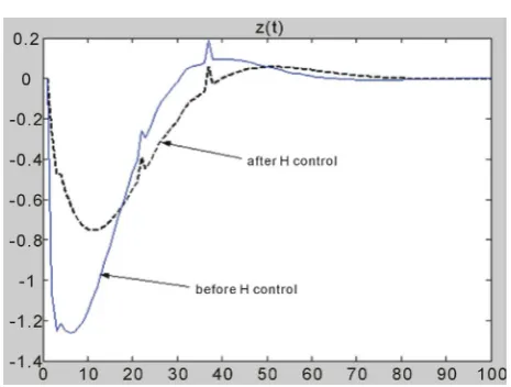
response trajectory is as dotdashline shown in Figure 2. Before and after optimization control, the system expectation output is as blue solid line and black dotted line shown respectively in Figure 3.

The system simulation shows that the disturbance attenuation degree

γ

can decrease to 0.0591 from 35.9133 after H∞ optimization control, and the anti-interference

performance is enhanced markedly. As a result, the system stability performance has been improved.

5. Conclusion

[image:10.595.309.539.339.523.2]

In this paper, when focused on network communication

[image:10.595.308.541.543.719.2]

Figure 2. State response simulation.

(11)

characteristics and singular plant characteristics si- multaneously, the H∞ optimal control problems for a

class of SNCS are addressed with both state feedback case and dynamical output feedback case. The network communication characteristics include the network-induced delay less than or equal to a sampling, limited input disturbance, clock-driven sensors as well as event- driven controller and actuators. The singular plant characteristics include impulse behavior, structuralinstability and something like that. This paper presents respectively the H∞ optimal control method, the existence condition

of H∞ control law and the solving method of H∞

control law and disturbance attenuation degree. The simulation results show that H∞ optimal control of

SNCS makes the disturbance attenuation degrees decrease obviously and makes the anti-interference performance enhance obviously. Therefore, the analytical method and the results are valid and feasible.

Acknowledgements

This project was supported by the National Natural Science Foundation of China (61074029, 61104093) and the Science Research Program of Liaoning Province (2011216007).

REFERENCES

[1] W. Zhang, M. S. Branicky and S. M. Phillips, “Stability of Networked Control Systems,” IEEE Control Systems Magazine, Vol. 21, No. 1, 2001, pp. 84-99.

http://dx.doi.org/10.1109/37.898794

[2] F. Y. Wang and C. H. Wang, “On Some Basic Issues in Networked-Based on Direct Control Systems,” Acta Au- tomatica Sinica, Vol. 28, 2002, pp. 171-176.

[3] Z. Wang and H. J. Gao, “Dynamics Analysis of Gene Regulatory Networks,” International Journal of Systems Science, Vol. 41, No. 1, 2010, pp. 1-4.

http://dx.doi.org/10.1080/00207720903477952

[4] H. J. Gao, T. W. Chen and J. Lam, “A New Delay System Approach to Network-Based Control,” Automatica, Vol. 44, No. 1, 2008, pp. 39-52.

http://dx.doi.org/10.1016/j.automatica.2007.04.020 [5] C. Jiang, D. Zou, Q. L. Zhang, et al., “Quantized Dynamic

Output Feedback Control for Networked Control Sys- tems,” Journal of Systems Engineering and Electronics, Vol. 21, No. 6, pp. 1025-1032.

[6] M. Liu and J. You, “Observer-Based Controller Design for Networked Control Systems with Sensor Quantization and Random Communication Delay,” International Jour- nal of Systems Science, Vol. 43, No. 10, 2011, pp. 1-12. [7] M. Liu, Q. Wang and H. Li, “State Estimation and Stabi-

lization for Nonlinear Networked Control Systems with Limited Capacity Channel,” Journal of the Franklin In-

stitute, Vol. 348, No. 8, 2011, pp. 1869-1885. http://dx.doi.org/10.1016/j.jfranklin.2011.05.008

[8] W. Yang, M. Liu and P. Shi, “H_∞ Filtering for Nonli- near Stochastic Systems with Sensor Saturation, Quanti- zation and Random Packet Losses,” Signal Processing, Vol. 92, No. 6, 2012, pp. 1387-1396.

http://dx.doi.org/10.1016/j.sigpro.2011.11.019

[9] H. Dong, J Lam and H. J. Gao, “Distributed H_∞ Filter- ing for Repeated Scalar Nonlinear Systems with Random Packet Losses in Sensor Networks,” International Jour- nal of Systems Science, Vol. 42, No. 9, 2011, pp. 1507- 1519. http://dx.doi.org/10.1080/00207721.2010.550403 [10] M. Liu, P. Shi, L. Zhang and X. Zhao, “Fault-Tolerant

Control for Nonlinear Markovian Jump Systems via Pro- portional and Derivative Sliding,” IEEE Transactions on Circuits And Systems—I, Vol. 58, No. 11, 2011, pp. 2755-2764.

[11] J. Li, Q. L. Zhang, H. B. Yu, et al., “Real-Time Guaran- teed Cost Control of Mimo Networked Control Systems with Packet Disordering,” Journal of Process Control, Vol. 21, No. 6, 2011, pp. 967-975.

[12] J. Li, H. B. Yu, D. Yuan, et al., “Co-Design of Networks and Control Systems with Synthesized Controller,” In- ternational Journal of Information and Systems Sciences, Vol. 7, No. 1, 2011, pp. 131-140.

[13] G. R. Duan, “Analysis and Design of Descriptor Linear Systems,” Springer, Berlin, 2010.

[14] Z. Z. Qiu, Q. L. Zhang and Z. W. Zhao, “Stability of Singular Networked Control Systems with Control Con- straint,” Journal of Systems Engineering and Electronics, Vol. 18, No. 2, 2007, pp. 290-296.

http://dx.doi.org/10.1016/S1004-4132(07)60089-9 [15] Z. Z. Qiu, Q. L. Zhang and G. Y. Li, “Output Feedback

Control Networked Control Systems Based on Singular Controlled Plant,” IEEE Proceedings of the 7th World Congress on Intelligent Control and Automation,Chong- qing, 25-27 June 2008, pp. 5463-5466.

[16] Z. Z. Qiu and Q. L. Zhang, “Exponential Stability for Sin- gular Networked Control Systems with Packet Dropout,” Control and Decision, Vol. 24, No. 6, 2009, pp. 837-842. [17] Z. P. Du, Q. L. Zhang and L. L. Liu, “Stability Analysis

for Singular Networked Control Systems with Time Vary- ing Delays,” Journal of Northeastern University (Natural Science), Vol. 32, No. 8, 2011, pp. 1065-1067.

[18] Y. F. Wang, Y. W. Jing, S. I. Zhang, et al., “Robust H_∞ Control for a Kind of Singular Networked Control Sys- tem with Short Time Delay,” Journal of Northeastern University, Vol. 32, No. 5, 2011, pp. 609- 613.