Current acceleration from the dilaton and stringy cold dark matter

Current acceleration from the dilaton and stringy cold dark matter

1_{Physics Department, McGill University, Montreal, Quebe´c H3A 2T8, Canada} 2_{NORDITA, Copenhagen, Blegdamsvej-17, DK-2100, Denmark}

(Received 20 October 2005; published 5 September 2006)

We argue that string theory has ingredients to provide us with candidates for cold dark matter and explain the current acceleration of our universe. In any generic string compactification the dilaton plays an important role, as it couples to the standard model and other heavy nonrelativistic degrees of freedom such as string winding modes and wrapped branes, which we collectively call stringy cold dark matter. These couplings are nonuniversal, which results in an interesting dynamics for a rolling dilaton. Initially, it can track radiation and matter while beginning to dominate the dynamics recently, triggering a phase of acceleration. This scenario can be realized as long as the dilaton also couples strongly to some heavy modes. We furnish examples of such modes. We provide analytical and numerical results and compare them with the current supernovae result. We also mention some of the challenges for the success of our model favoring certain stringy candidates.

DOI:10.1103/PhysRevD.74.063501 PACS numbers: 98.80.Cq

I. INTRODUCTION AND SUMMARY

If string theory is the right paradigm for quantum grav-ity, then it must provide us with all the ingredients to make the currently observed universe. According to the most recent measurements [1], the universe is, to a good ap-proximation, spatially flat, and the current energy budget of the universe consists of about 30% nonrelativistic matter, most of it being weakly interacting and known as cold dark matter (CDM), and about 70% is in the form of an un-known source of dark energy which is responsible for the current acceleration. Unless a dominant fraction of them is hidden in dark astrophysical objects, standard model (SM) baryons can only make up a small fraction of the total energy density.

Obtaining the SM sector from string theory has been a hot pursuit; for a review, see [2]. However, in making the present universe, it is equally challenging to seek a candi-date for cold dark matter which cannot be otherwise ex-plained within the SM [3]. Finally and most importantly, one also has to obtain the vacuum/dark energy which seems responsible for the current acceleration [1,5].

Now it is well known that any string and/or supergravity compactification to four space-time dimensions usually [6,7] leads to a runaway potential for the dilaton (see [8] for efforts to stabilize the dilaton). Let us study the rolling dilaton dynamics in light of the dilaton’s coupling to various matter fields. It is important to realize that the dilaton does not have a universal coupling to all the matter degrees of freedom [9], and it is this fact that we are going to exploit in our paper [10]. In order to have a holistic cosmological evolution in our model, we would require the following ingredients:

(1) The CDM candidate should be treated on an equal footing as the SM baryons in order to explain why B=CDMO1. Therefore, if we assume that the

dilaton couples to both the sectors, then it should

have a similar coupling. In summary, both the SM and the CDM components should couple weakly (or be uncoupled) to the dilaton, in order to comply with various empirical constraints from fifth force experi-ments, from observational bounds on the variation of the fine structure constant and of Newton’s con-stant, etc.

(2) In order to explain the current acceleration, we further require another CDM sector which is strongly coupled to the dilaton, and which we coin SCDM. We will see that, by virtue of its coupling to the dilaton, SCDM redshifts much more slowly than CDM and therefore may dominate the matter energy density at late times even if it was subdominant at early times. Moreover, if the coupling is strong enough, it slows down the rolling of the dilaton, causing the energy-momentum tensor of the dilaton to lead to an accelerated expansion of the universe. We will provide examples of both standard CDM and SCDM in the context of string theory. Introducing a new form of dark matter may lookad hocat first glance, but as we shall see such states are already present in string theory. Moreover, our approach to explaining dark energy has an obvious advantage: no new extremely light, m 1033 _{eV, scalar field is required to explain the origin of}

dark energy unlike in quintessence models [11–13] (for alternative explanations, see [14]). The natural scale in our approach is solely governed by the string scale. In this respect our model is minimal and facilitates making con-nections to string theory. The reason why acceleration starts at a much lower scale than the Planck scale, as we argue, can be traced back to having small initial cosmo-logical energy densities of SCDM string states in the early (post-inflationary) universe.

string and brane degrees of freedom we make use of (which are the same ones studied in brane-gas cosmology [15,16]; see also [17]) couple to the dilaton, and give examples of candidates for SCDM which couple to the dilaton in a way which can give rise to acceleration. In Secs. III and IV, we provide analytical and numerical descriptions, respec-tively, of the evolution of the four distinct components in our cosmology, namely, radiation, CDM, SCDM, and the dilaton. We also constrain the couplings by fitting to the supernovae data. In Sec. V, we readdress the cosmic accel-eration problem within the string theoretic framework. We conclude by summarizing and pointing to future research challenges.

II. MOTIVATION FROM STRING THEORY

A. Dilaton gravity

The main aim of this section will be to find two impor-tant couplings, first the dilaton self-coupling which will determine the slope of the runaway potential, and second the coupling of the dilaton to the stringy degrees of free-dom, allowing us to identify stringy candidates for CDM and SCDM.

Let us start with 10-dimensional type II string theory whose low energy bosonic action is given by

^ SII

1 16G^

Z

d10_xp_g

e2

^

R4@m^@m^V

1 12H

2 3

X

n

ean 1 2n!F

2

n

; (1)

where hatted quantities denote the full higher (D^ 10) dimensional objects, is the dilaton, H₃ is the field strength of the antisymmetric tensor field, and the field strengths Fn’s are n forms (where n2, 4 in type IIA theory whilen1, 3, 5 in type IIB theory). To be general, we have also added a potential for the dilaton. Such a potential could result from quantum corrections [6,7].

We will assume that all shape and volume moduli of the internal manifold are stabilized. This could occur by mak-ing use of the GKP scenario [19] to stabilize the complex structure (shape) moduli with the help of various form fields, and then invoking the KKLT ideas [20] to stabilize the volume modulus with the help of nonperturbative processes. Alternatively, but only in heterotic string theory, we could use ideas from brane-gas cosmology [15,16] to stabilize both volume [21–23] and shape [24] moduli by means of string states which are massless at the self-dual radius (see also [25] for a study of volume stabilization in the string frame which is applicable both to type II and heterotic string theories). We assume that these moduli do not play any substantial role in the late-time dynamics (this assumption is supported by the analyses of [22,23]), and henceforth we will ignore them.

Performing the well-known conformal transformation (relating the string-frame metric on the left-hand side to

a function of the dilaton multiplying the Einstein frame metric on the right-hand side)

^

g_m^n^ !e4=D

2_g^

^

mn^; (2)

(where D

is the number of compactified spatial dimen-sions), we recover from (1) an action in the 10-dimensional Einstein frame,

^

S 1

16G^ Z

d10_xp_g^

^ R1

2@m^@

^

m_2V

;

(3)

where the new potential is related to the original one by rescaling:

V !e=2_{V: (4)}

We take the full higher-dimensional metric to be

^

g_m^n^ gmnx 0 0 r2_g

mny !

; (5)

where r is the radius (volume) modulus of the compact space and where we used the symbol ‘‘’’ to indicate extra-dimensional quantities.

Then, after integrating over the extra dimensions, one straightforwardly obtains

SM

2

p 2

Z

d4_xp_gR@

m@m2V ; (6) where we have defined

M2

pM8sr6 (7)

as the four space-time – dimensional Planck mass, and we have also rescaled,

! 1 2

q

; (8)

so that it has a canonical kinetic term.

As in [26], we now specialize to the case whenVis an exponential potential,

V V0e2: (9)

Indeed, such exponential potentials are common in lower-dimensional supergravity models and can also arise in string theory from quantum corrections (both perturba-tively, for example, involving string loops [6,9], or non-perturbatively, like in gaugino condensation [7]). Although we keep as a free parameter in our model, ideally one should be able to derive its value from the origin of the potential, and we discuss an example in Sec. V.

B. Wrapped branes as candidates for CDM and SCDM

special modes which are massless at the self-dual radius — however, such modes exist in heterotic theory but not in type II string theory). The dilaton, in general, couples to these objects, and here we determine these couplings. As in the usual brane-gas cosmology paradigm [15,16], we as-sume that branes have annihilated in the three noncompact directions, allowing them to expand, and leaving us only with branes wrapping some or all of the six internal extra dimensions. Hence we only need to compute the couplings forp-branes withp2;. . .;6, and for the string winding and momentum modes.

The brane couplings can be derived [27,28] starting from the Dirac-Born-Infeld (DBI) action, which in the string frame reads

SDBIMp

1

s Z

dp1_ep_{; (10)} whereis the metric on the brane world sheet labeled by . One has to now make conformal transformations (2) followed by dilaton rescaling (8) to obtain the brane cou-plingpin the Einstein frame:

S_DBIMps1 Z

dp1_e2pp ₍₁₁₎ with

2_pp3 8

p : (12) The wrapped branes of course appear to us, from the large four space-time –dimensional point of view, as pointlike objects. Thus, their number density redshifts as a3, like nonrelativistic dust. In the brane-gas approximation the four-dimensional action for wrappedp-branes is therefore given by (see e.g. [22])

S_brane Z d4_xp_g

0e2p

_a

a₀ 3

Z d4_xp_g~

p;

(13)

where ~p corresponds to the observed four-dimensional energy densities of the wrapped branes which appear in the Einstein equations [29]. Note that, because of the coupling, ifpis positive the energy density~predshifts slower than a3_{if the dilaton increases, and this is why these wrapped}

branes can act as candidates for SCDM.

By an analogous prescription we can also obtain the four-dimensional action for string winding modes [30], and momentum modes starting from the Polyakov action [31]. For the winding modes we find

2₁ 1 2

p ; (14) while the momentum modes do not couple to the dilaton at all [31]:

mom0: (15)

One immediately realizes that, since the momentum string modes do not couple to the dilaton, their energy density redshifts in the same way as baryons, i.e. asa3_,

and therefore they can be candidates for CDM. On the other hand, the coupled winding states can form SCDM. However, since we want SCDM to become important (comparable to CDM) only at the present cosmological epoch, this means that in the early universe the energy density of the winding states must have been much smaller than that of the momentum modes. Here, we present a qualitative argument based on the masses of these objects as to why we expect this to be the case. We will address the issue more quantitatively in Sec. V B.

From Eq. (12) we can directly read off the masses of the p-branes as

m_pMps1rp; (16) whereris the radion field in the Einstein frame. We assume that the radion is stabilized. Similarly, from the Polyakov action the masses for the string winding and momentum modes are given by

m1M2sr; (17)

and

mmom

1

r: (18)

For the purpose of illustration, here we have assumed that, initially, evolves from close to zero, but similar argu-ments can be made for more general initial conditions.

If the radion is stabilized at a scale slightly lower than the Planck scale, sayr1_M

GUT, then, because of ther

dependence of the different masses, the momentum modes turn out to be the lightest, while all the winding string modes and branes are much heavier. Thus, if there was a period of inflation of the three large spatial dimensions, and if the temperature after reheating is of the GUT scale, then the reheating process at the end of inflation can either perturbatively [32,33] or via parametric resonance [34,35] produce string momentum modes [36]. The thermal pro-duction of the winding states (which are very heavy com-pared to the scale of inflation) is exponentially suppressed. There are, however, some mechanisms by which such heavy modes could be produced [38,39], although their number densities would be much smaller than that of the momentum modes. Thus, in the context of inflationary cosmology, this may yield one way to explain the differ-ence in the initial post-inflationary energy densities of the momentum string modes (CDM) and the winding modes (SCDMs). It is possible, however, that the winding mode production processes after inflation are too weak. In this case, one must invoke the primordial preinflationary den-sity of SCDM states to determine the late-time number density: in Sec. V we argue how a period of inflation of appropriate length can dilute primordial energy density of

SCDMs to make it just right to address the coincidence problem.

If both baryons and CDM momentum states are pro-duced during reheating after inflation, then it should be expected that their densities are comparable, as long as the masses of both types of states are small compared to the typical energy scale during reheating. If the initial post-inflationary baryon density is not changed substantially by later stages of baryon production, the number densities of baryons and CDM particles are expected to be comparable. Let us then assume that after inflation we have very small energy densities of the different wrapped brane/ string gases. Now observe that, because of the difference in the coupling exponents p’s, all the species redshift differently. Asis increasing, it is clear that very soon the largest energy density among these different species would correspond to the one with the largest positive p. From (12) and (14), one finds that this corresponds to the 6-branes, with

6

3

2p8: (19)

Thus, according to our scenario, at late times the dark sector of our universe will consist of three main compo-nents: (a) the dilaton behaving as dark energy, (b) string momentum modes playing the role of ordinary CDM, and (c) 6-branes, which wrap the six extra dimensions, playing the role of SCDM. As we shall see in the next section, by virtue of their coupling (19) to the dilaton, 6-branes can trigger a late phase of acceleration.

III. COSMOLOGICAL MODEL

A. Acceleration due to coupling: basic mechanism

We begin by analyzing a simple scalar-tensor theory action for dilaton gravity, where the dilaton has a runaway potential:

SgravM2p Z

d4xpg _R

2 @2

2 V0e

2_:

(20)

In principle,can be identified with any suitable moduli field, as exponential potentials are quite common for other kinds of moduli fields as well, for example, in flux com-pactifications [40]. However, for the purpose of this paper we focus on the dilaton. As in conventional cosmology, gravity is sourced by the matter-radiation stress energy tensor which can be derived from an action of the form

S_iZ d4_xp_g~

i; (21)

where the indexi represents the different components of matter/radiation and~iis the observed energy density that gravitates. The Hubble equation reads

H2 1

3 X

i ~ _i1

2 _

2V

1

3 X

i ~ _i~

: (22)

Note there is a departure from the conventional cosmology. We allow different matter components to couple to:

~

ie2ii; (23)

where we further assume that the -independent ‘‘bare density’’ _i behaves like a perfect fluid, i.e., it obeys the continuity equation:

_

_i3Hp_ii 0; (24)

with an equation of statep_i!_ii.

If a scalar fieldis to act as a quintessence type field, then it must be virtually massless, i.e.m1033 _{eV. If}

is coupled to SM particles, it mediates a fifth force. Fifth force experiments constrain such couplings of to SM degrees of freedom to be very small, SM<104–105

(see e.g. [41]). Observations on variation of physical con-stants like the fine structure and Newton’s concon-stants also give us similar bounds on_SM. To be able to explain such small couplings is, in fact, a generic and challenging problem in quintessence models. However, one finds that in our specific scenario where the dilaton evolves to a strong coupling regime (1) such small couplings may have a natural explanation [42], as discussed in [6]: In this setup one expects the masses, mb’s, and gauge couplings,g’s, for standard model particles to be given by a Taylor series expansion in inverse string coupling (gs1e) [6]. For example, if GUTis the GUT-scale

fine structure constant, then we have

GUT01e : (25)

Now, the crucial thing to note is that observations really only constrain the dimensionless ratios

1 m_b

dm_b d ;

1 g

dg gd<10

4_–105_:

For large values of, one can easily estimate these quan-tities. For instance, from (25)

1 _GUT

d_GUT

d

₁e 0

e_{: (26)} Thus, as long as the constant term in the expansion is nonzero (in general, it is nonzero, and is determined by the various group theoretical quantities of the gauge group [6]) the ratio becomes smaller and smaller asevolves to larger values and one can easily satisfy the observational bounds.

which do not necessarily conform to the perturbative ex-pansions such as (25), potentially invalidating our argu-ment. However, a detailed study of these effects is well beyond the scope of our paper and we will assume that (25) is valid, at least in some parameter range. We have dis-cussed this issue in the Appendix.

Therefore, in the following we will assume that radiation (r), baryons (b), and CDM (string momentum modes) have tiny/no couplings to.

The dynamics ofdepends on the exponent, and the coupling ofto various matter-radiation components. The equation of motion foris given by

3H_ V0

eff; (27)

with

Veff V0e2

X

im;sc

e2i

i; (28)

where the sum runs over all matter states. For simplicity, we have assumed that the gauge bosons do not contribute to an effective potential for . This is strictly true if, on average, the electric and magnetic fields vanish. There could be other forms of radiative matter which could induce an effective coupling, as discussed, for example, in [44]. Weakly coupled matter (stringy candidates for CDM and baryons) are denoted by the subscript ‘‘m,’’ and SCDM by the subscript ‘‘sc.’’

It was argued in [26] that, when the universe evolves adiabatically, the dilaton tracks the minimum of the effective potential which evolves in time with the redshift-ing of the i’s. How fast or slow the dilaton is evolving mostly depends on the equation of state parameter!_i, and on the coupling exponent _i of the dominating matter component. Thus, at earlier times when radiation or weakly coupled matter is dominant,rolls fast and tracks the relevant matter/radiation component, remaining sub-dominant. However, once SCDM becomes important, the dilaton slows down, starts to dominate the energy density, and our universe enters a phase of acceleration. Let us now see this in more detail.

B. Exact two-fluid analysis

We will first work within the approximation that there are only two dominating components in the universe, the dark energy determined byand a single matter/radiative component. To keep things general, we do not specify which form of matter it is. In this approximation, the Einstein constraint equation (22) determining the Hubble expansion rate reads

H21

3e2

1

2_

2_{V: (29)}

From Eq. (27), it follows that the evolution equation for is given by

3H_ 2V₀e2_e2_{: (30)}

Solving the continuity equation (24), we obtain

0

_a

a0

31!

(31)

where0 is the present-day value of the energy density.

Performing a change of variables lnatleaves us with the following set of equations:

H2 1

3e

2_V

0e2

11

6

02 ;

00

3H

0

H

02V0 H2e

2₂

H2e

2_;

where 0 d=d . The system of equations can be solved analytically to obtain the ‘‘tracking solution,’’ the solution where ttracks the minimum of its ‘‘effective’’ poten-tial. The solution is given by

e V0

_3=41!

3=41!2_3=81!

p

(32)

where

p 1

2 (33)

and

at a0

_t

t₀

₂₌31!

with!

=!

=1:

(34)

A few remarks are now in order. First, we observe that the energy densities ~ and ~ track each other and redshift with precisely the same equation of state parameter ! that was derived in the adiabatic approximation in [26]:

~

3=41!2_3=81!

3=41! ~

r~a31!_: (35) One recovers the value of the tracking ratio

r

; (36)

obtained in the adiabatic approximation [26] when;

O1and the terms involving1!can be ignored. Second, we realize that real solutions foronly exist if the numerator on the right-hand side of (32) is positive (the denominator is positive as long as ! >1=2). In other words, in order for a tracking solution to exist, we require

>31!

4 : (37)

Since we want such tracking behavior to hold during the radiation-dominated phase, substitutingr0and!r 1=3in Eq. (37), we find

>1: (38)

We note in passing that, if the condition Eq. (37) is not satisfied, then we end up with a different, nontracking, late-time attractor solution. In this case the field does not follow the minimum but lags more and more behind as the uni-verse expands, and the energy density becomes dominated by the dilaton from the very beginning. From the point of view of cosmology, this is an uninteresting scenario.

Finally, we find from Eqs. (34) that acceleration happens when

sc

> 3 2

₁

3!sc

: (39)

For winding brane SCDM (!_sc0), combining (39) with (38), we find that we can account for a late acceleration phase provided our SCDM has a coupling exponent,

sc>1₂: (40)

Note, in particular, that the exponent which we computed for wrapped 6-branes satisfies this bound.

C. Three-fluid system

Our exact analysis of the two-fluid model suggests that, if the dilaton couples to SCDM, then there can be an interesting dynamics which triggers a phase of accelera-tion. In order to study more precisely how such a transition happens, one has to consider a more realistic cosmological model where, in addition to the SCDM fluid, we also have a normal CDM component that is uncoupled or weakly coupled to the dilaton. Such a model has the advantage that, at early times, the evolution is standard, i.e. H a3=2, and, at late times, as SCDM plus dark energy begin to dominate, we can have accelerated expansion.

The new system of equations (22) –(27) becomes

H2 1

3M2

p

~~_sc~_m; (41)

3H_ 2V₀e2scsce2scmme2m 2V _sc~_scm~_m : (42) For simplicity, we assume for the time being thatm 0; we will see later that, as long as_m, it hardly makes any difference to our analysis. Although no analytical solution to Eqs. (41) and (42) is found, one can obtain some insight into the cosmological evolution resulting from these equations by considering various limiting situations.

First transition. —First, consider a situation when the energy density in SCDM is much smaller than that in both ordinary matter and inV, so that one can neglect the second terms in Eqs. (41) and (42). In this case, the equations from the two-fluid discussion apply, making use of0andw0. This is the phase when the dilaton

essentially rolls down freely along its potential V, tracking the energy density of ordinary matter [26] as given by (35):

~

3

82₆~m: (43)

The scale factor at /t2=3_{, as in the usual}

matter-dominated era. Note that during this period the value of which is the minimum of the ‘‘effective potential’’ for [the sum ofVand~sc] is redshifting more slowly than

the value oftin this phase [this can be seen by going back to (32), since it is setting sc in this equation

which gives the time dependence of the minimum], and thus t eventually catches up with the minimum. After this point, the value of t tracks the minimum. In this case, we know that the energy density of will track SCDM, as given in Eq. (35). It is clear, then, that when the right-hand sides of Eqs. (35) and (43) become equal, i.e. when

3

423~m

~sc (44)

and thus

~ sc

3

42₃~m; (45)

a first transition, namely, the transition between the period whentis moving freely and when it starts tracking the minimum of the effective potential (set by the interaction of the dilaton potential and the contribution from the SCDM term), occurs [45]. From this moment on, both

~

_sc and~_Q start to redshift as Eq. (35), with!!0and !_sc.

Second transition.—The second transition [46] corre-sponds to when the universe enters a phase of acceleration. This happens approximately when~_d ~_sc~ 1 rsc~scbecomes equal to the energy density of the ordinary

matter components, as can be readily seen from the Hubble rate, Eq. (41). Thus, we enter a phase of acceleration when

~ sc

1 1rsc

~

_m 1

1sc=

~

_m; (46)

where in the last step we again made use of the adiabatic approximation.

First, notice that, depending on how large the ratio _sc=is, one needs a very small fraction of SCDM com-pared to ordinary weakly coupled matter to initiate the phase of acceleration. Since SCDM behaves like nonrela-tivistic dust (!sc0) it would cluster around galaxies and

galaxies (at recent redshifts), it is important that this ratio does not change too much in our model. This is guaranteed if~_scis only a small fraction of~_m. As pointed out in [26], this scenario of changing baryon to dark matter abundance offers the intriguing possibility of reconciling a 10% to 20% discrepancy in the estimates of baryonic abundances coming from CMB and big bang nucleosynthesis (BBN) measurements [47].

What if SCDM is a radiative fluid?—So far, we have assumed that SCDM is a form of dark matter (winding states) but is strongly coupled to the dilaton. What if it were to behave as a radiative fluid? For example, in [44] it was proposed that thermal fluctuations of a massless field with quartic interactions can act as a radiative fluid with pre-cisely the kind of exponential coupling to the dilaton that we considered here. In this case, !_sc1=3, and we will observe it as a component of dark energy. This is because, after the first transition, both SCDM andobey the same equation of state!as computed in Eq. (35), and cosmo-logically we cannot distinguish between the two. The total dark energy would then be given by~d. Obviously, in this setup the ratio between dark matter and baryons remains constant and we do not encounter any constraints on the ratio_sc=on this basis. From (39) we find that in order to have acceleration the ratio just needs to satisfy

>1: (47)

Acceleration epoch.—In either case, the main constraint comes from trying to match the observed equation of state, !<0:76 [1,5]. From Eq. (34) we find such a bound implies

sc

>3 (48)

for SCDM and

sc

>5 (49)

for radiation. How to get such a large value of the ratio from string theory is discussed in the following section.

For these ratios of_sc=, one can also estimate approxi-mately the onset of the period of acceleration. It is the time when~_d~_m. Now,

1 ~d;acc ~ m;acc

~d0 ~ m0

_a

acc

a0

3!Q d0

m0

₁

1zacc

3!Q :

(50)

Using the known dark matter to dark energy ratio, we find

zacc0:5–1:0; (51)

which is in good agreement with the supernova data.

Finally, we note that most of our analyses of the tran-sitions go through identically even if _m is nonzero but small. This is because, if_mis tiny, it changes the tracking ratio very little in the matter phase (43), which enters in the calculation for the epoch of the first transition. Also,

~

ma3Om=:

Thus, weakly coupled matter redshifts essentially the same way as in the standard cosmology, and therefore the second transition is also unaffected.

To summarize, we have three distinct cosmological eras depending on which terms are most dominant on the right-hand side of the Hubble equation (41):

(1) The radiation era, when~_sc and~_m are negligible while~tracks~_r;

(2) The matter era, when~scand~rare negligible while ~

tracks~m;

(3) An acceleration phase, where stringy components, viz.~d, start to dominate over~m.

As far as the parameters of our model are concerned, first we find that, in order to have a late-time acceleration phase, we need the ratio sc= to satisfy conditions like

Eq. (62). On the other hand, to have an earlier nonaccel-erating phase _r; _m has to be small which is consistent with constraints coming from fifth force experiments, and observations of variation ofG_N and_f which lead to the condition SM<105. Finally, the requirement that

should track radiation in the early universe tells us that > 1. In spite of these constraints, there is a huge parameter space where we seem to agree with the cosmological and particle physics observations, which is encouraging. Let us therefore study this model in more detail using numerical techniques and see whether the allowed parameter space can be made more precise.

IV. NUMERICAL WORK

A. Evolution and abundances

In order to verify our analytical approximations and see the precise evolution of the system, we solve the three-fluid system numerically. We start deep in the matter-dominated era and choose initial conditions such that the field initially follows the approximate early-time solution. As an ex-ample, the evolution of the field for the set of parameter values 6, 10, _m~ 0:27, _m0:01, and V₀ fixed by requiring flatness is shown in Fig. 1. The plot depicts the field value as a function of time (measured in terms of the logarithm of the scale factor). The solid red curve represents the full numerically determined evolution. In the same figure we also show the analytical approxima-tions given by Eqs. (41) and (42) in a universe that is radiation dominated, i.e.exp 82_V

0=3r1=2 (dot-dashed purple curve), dominated by ordinary matter, i.e. exp 82V0=3 ~m1=2(long-dashed green curve), or described by the late-time solution (dashed blue curve)

when the field follows the effective minimum of the po-tential Eq. (35). From the figure, one can see how the field initially follows the radiation-dominated solution until it crosses the matter-dominated solution, after which the evolution of the fields is well described by it. At late times, the field follows the solution of the evolution of the mini-mum of the effective potential. Note also how the crossover from one solution to another is very rapid and smooth.

The relative contributionsiof various matter constit-uents (labeled byi) to the critical density of a spatially flat universe are shown in Fig.2. It is clear how at late times the

coupled dark matter component starts dominating along with thefield.

B. Observational constraints: Supernova type Ia data

In order to see whether the model presented here is compatible with present observational data, we compare it with the recent expansion history as probed by the supernova type Ia (SNIa) data. Here we use the sample of 194 SNIa presented in [48]. In order to compare our model with theCDMmodel, we compute the2_{for each}

set of parameters and compare it with the value for the corresponding flatCDMvalue, which for the same set of supernovae is 2_CDM201:6(_m 0:27, 0:73).

The contribution from radiation is neglected for the SNIa fit, and the universe is assumed to be flat. The Hubble parameter is marginalized over in all of the fits (by max-imizing the likelihood).

In Fig.3we show a contour plot of coefficients; corresponding to 2 22

CDM, where we have

fixed _m 0:27,_sc0:01. The region above the blue (short-dashed) curve shows where the 2 _{is smaller than}

2

CDM, indicating a nominally better fit to the data. The

green and red curves indicate contours where 2 _{is 2}

and 4, respectively. The reduced 2 _{for the CDM}

model is 201:6=1941 1:045, so an equal reduced 2 _{is achieved with the model considered here (with two}

extra parameters), when2 _2:1.

The dependence on the coupled matter parameterscis

very weak, whereas the uncoupled component plays a significant role. For example, with large values, m 0:4, the contours shift such that all of the considered ; parameter space gives a larger2 than theCDM value. Small values, m0:2, lead to the same conclu-sion. In this section, our main purpose is to demonstrate the

0 0.2 0.4 0.6 0.8 1

-6 -5 -4 -3 -2 -1 0

Ω

log(a)

FIG. 2 (color online). The relative energy densities in the

field (red solid line), in coupled CDM (SCDM) (blue dashed line), uncoupled CDM (green long-dashed line) and in radiation (purple dot-dashed line).

0 5 10 15 20 25

1 1.5 2 2.5 3 3.5 4 4.5 5 5.5 6

µ

β

FIG. 3 (color online). Contour plot of2₍ ~

m0:27,m

0:01). The red (solid) contour corresponds to 4, the green (long-dashed) contour to 2, and the blue (short-dashed) con-tour to 0.

-0.7 -0.6 -0.5 -0.4 -0.3 -0.2 -0.1 0 0.1 0.2 0.3

-6 -5 -4 -3 -2 -1 0

φ

log(a)

properties of the model considered here and to show how it can fit the current SNIa data very well. A more complete parameter scanning is left for future study.

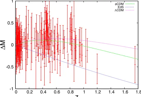
In order to understand qualitatively why2_{is negative}

for a range of parameter values, we show the luminosity distance plot as a function of redshift with respect to the empty universe, M, for a set of parameters (1:3, 8), for which22_CDM 4:2, in Fig. 4. From the figure, we see how for these parameters the luminosity distance at low redshifts closely follows that of theCDM but, at later times, curves down more quickly, fitting the high redshift data points better.

V. STRINGY PHYSICS AND COSMIC ACCELERATION

Although we have seen that stringy SCDM can pave the way for a late-time acceleration phase, challenges remain to connect string theory with our coupled quintessence model in a quantitative way. First, our numerical analysis involving supernovae data suggests that we require= 2and 1:4 for a good fit. The parameters are further pushed up if one also considers bounds coming from BBN: During the radiation era (r0) we have

~

5

62₁~r: (52) BBN considerations provide an upper bound on the dark energy abundance, <0:21 during the radiation era. From Eq. (52) we see that for this to be satisfied one needs >2.

Second, it is clear that the success of our cosmological scenario relies on having a very small abundance of CDM and SCDM in the early universe, and it would not be much progress if we simply shift the usual problem of

quintes-sence models, namely, the problem of having to invoke a new and extremely small mass hierarchy (namely, the eV mass scale), to a problem of an unnaturally small initial abundance of the SCDM particles. Thus, in order to truly address the cosmic acceleration issue one needs to explain quantitatively why we expect such small abundances. In this section we address both of these issues, starting with the first.

A. Quantum stringy corrections

One may argue that we can obtain the required values of ; if stringy SCDM is coupled to several scalar fields [49]. This is because, depending upon which linear combi-nations are stabilized, the effective for (the linear

combination which is rolling) can range from 0 to P_I2

I q

, whereI’s are the exponents of the couplings to the differ-ent scalar fields, I’s. Analogous arguments hold for . However, rather than invoking many scalar fields, here we furnish an example which shows how quantum corrections involving stringy loops may be able to provide us with a significantly large value of.

In the string frame, quantum string loop corrections will, in general, modify the couplings of the dilaton to the different fields:

SZ d10_xCRK@2_{V ; (53)}

where the functionsC,K, andVare expected to have a Taylor series expansion in terms of the inverse string coupling constantg1

s e[6],

C X

1

n0

C_nen_{; (54)}

and similarly forKandV. We recover the classical action (1) when all coefficients, exceptC21andK2

4, vanish. Now, let us suppose that the first nonzero coef-ficients of C and K occur at the nth level, while V₀ 0[53]. Then, as! 1, the action is given by

SZ d10_xen_Ren_K

n@2V1e : (55)

To go to the Einstein frame, we perform a conformal transformation,

^

gm^n^ !e2n=D

2_g^

^

mn^; (56)

followed by rescalings,

!

n2_{D 3}

D

2 Kn v

u u u

t k; (57)

to make the kinetic terms for the dilaton canonical. After dimensional reduction to four dimensions, the action reads -1

-0.5 0 0.5 1

0 0.2 0.4 0.6 0.8 1 1.2 1.4 1.6 1.8

∆

M

z

φCDM EdS

ΛCDM

FIG. 4 (color online). Luminosity vs distance with respect to the empty universe for 1:3; 8 (green long-dashed line), the CDM model (purple dot-dashed line) and EdS (blue short-dashed line) along with the SNIa data.

S 1 16G

Z

dx4p_gR@

m@mV1e2 ;

(58)

where

2D

22n kD 2

: (59)

Next, we look at the DBI action for D

-branes and perform the conformal rescalings (2) to obtain the effective four-dimensional action for the gas of 6-branes:

Sbrane

Z

d4_xp_g~Z _d4_xp_g

0e2sc

_a

a0

3

;

(60)

with

sc

D

n1 n2 kD 2

: (61)

Note that we want=to be positive. SubstitutingD

6, one finds that this is possible only forn2, 3, 4:

for n2; sc 1;

for n3; sc

13

4 3:13;

for n4; sc 10:

From Eq. (57) it is also clear that, depending on the value ofKn,kcould be small, hence makingsc; large.

B. Primordial inflation and the scale of current acceleration

It is clear that a resolution of the dark energy problem should not only involve (a) a tracking mechanism which explains why the dark energy density has always been close to the matter density, and not just today (and this is most certainly the case in our model), but also (b) a pa-rameter (since we do not want to introduce a hierarchical eV mass scale) which governs when the dark energy comes out of the tracking phase and starts to dominate the uni-verse. Moreover, this parameter should be such that its expected value can naturally explain why we are entering this phase of acceleration so late in the day.

Now, in our model, acceleration commences approxi-mately when SCDM becomes comparable to ordinary CDM. Since SCDM redshifts more slowly than CDM, this means that in the early universe (say just after infla-tion) the energy density in SCDM was much smaller than that of CDM. This could happen, for example, if SCDM is

produced very scantily during the reheating process, as argued in Sec. II. More importantly, one realizes that SCDM candidates are stringy winding states in nature. One expects these winding states to be present in the very early preinflationary universe with approximately string scale energy densities. However, as our universe expands exponentially during inflation, this gas of branes is going to become very dilute. Since the slope of the potential decreases exponentially as increases, we ex-pect the dilatonto be effectively frozen during the phase of inflation. As a result, the SCDM energy density will redshift asa3.

Thus, at the end of inflation, while the energy density in ordinary matter would be given by the reheat temperature, the energy density in the primordial gas of SCDMs would be much smaller due to inflationary dilution. In fact, the larger the number of e-foldings,N, the greater the dilu-tion, and therefore the longer it will take for SCDM to catch up with CDM, and the smaller the scale (M_A) would be at which the second phase of acceleration com-mences. If MAMp10A, then one finds (see the Appendix for details)

AR14=3!sc 1:3N 271!sc 4=!_sc

(62)

whereM_P10R _{corresponds to the reheat temperature.} We are now in a position to estimate the scale at which the second acceleration phase starts. As a first example, let us choose !_sc0, and =1=2, the minimal value required for acceleration and also approximately what one obtains for the 6-branes. For the minimal number of e-foldings, N 60, and assuming reheating to GUT-scale temperatures Mreh, i.e. Mreh103Mp or R3, one finds from (62) that M_A1030_M

p102 eV. We remind the reader that the current energy density corre-sponds to the energy scale 103 _{eV. For !}

sc1=3, i.e.

radiative SCDM, one needs =1 for acceleration. Then, using previous values forN andR, we again find M_A1030_M

p.

The agreement, however, is not as dramatic as it seems. The more detailed numerical analysis performed with !sc0 revealed that we get good agreement with the

variation inN results in only a small variation inA. This is, of course, to be contrasted with the fine-tuning problem inCDMmodels where the difference of two large num-bers is supposed to yield a very small cosmological con-stant. Hence, a small variation in one of the large numbers causes a huge variation in.

VI. CONCLUSIONS

In this paper we have introduced the concept of ‘‘stringy cold dark matter’’ (SCDM). From the point of view of our four-dimensional space-time, SCDM are particles which couple nontrivially [with a coupling exp2] to the dilaton. Candidates for SCDM from string theory are branes wrapping some or all of the compact spatial dimen-sions. We have studied the cosmology of these modes in the context of a type IIA supergravity action to which we have added a runaway potential V0exp2 for the

dilaton (as explained in the text, such potentials are generally believed to be generated when going beyond the classical description). We have shown the existence of cosmological tracking solutions in the context of which the dilaton becomes a candidate for dark energy [54].

Our model contains radiation, regular dark matter (which couples very weakly if at all to the dilaton), SCDM, and the dilaton. Assuming that our four-dimensional space-time underwent a period of primordial inflation, the initial energy density in SCDM is expected to be exponentially suppressed compared to the density of regular CDM and radiation (which can be produced during reheating after inflation). In this context, the universe is initially dominated by radiation, and we show that the energy density in the dilaton tracks that of radiation until the dilaton gets stuck at the minimum of its effective potential, a potential formed from the dilaton potential (potential with a negative slope) and the terms with posi-tive slope coming from the interactions of the dilaton with SCDM. From then on, the density in SCDM and in the dilaton redshifts more slowly than that of ordinary matter. During this phase, the density in the dilaton is greater than that in SCDM. Once the dilaton energy begins to dominate, a period of acceleration begins, provided = is suffi-ciently large.

Compared to models of quintessence, an advantage of our approach is that it does not require the introduction of a new mass hierarchy (a new mass scale of about 1 eV). In order to explain why the late-time acceleration begins at the present time, a sufficient suppression of the number density of SCDM states is required. Such a suppression is naturally generated by a period of cosmological inflation. In fact, the numberN ofe-foldings of inflation required to suppress the SCDM density is (for GUT-scale reheating) larger but of the same order of magnitude as the minimal value ofN required for successful inflation. Thus, in our framework the ‘‘coincidence mystery’’ of why dark energy

is beginning to dominate today is tied to the duration of the period of inflation.

For our scenario to work, a sufficiently large value of = is required. Even larger values of this ratio are required to be consistent with big bang nucleosynthesis. At the level of the classical action, it is not possible to obtain such large couplings between the SCDM particle and single scalar moduli. The cumulative effect of cou-pling the SCDM particle to several different scalar fields may help resolve this difficulty, as may nonperturbative effects. Further research on this issue is required. A proper understanding of 0 and string loop corrections is also necessary in order to study the stability of this model; we have assumed the validity of Ref. [9] in the low energy regime we are interested in. It is an important task to have known these corrections to all orders; however, this is not the main focus of this paper.

It would be interesting to study further consequences of the existence of SCDM in the present universe, following the approaches of [56] to study cosmological consequences and of [57] to study astrophysical and particle physics aspects.

ACKNOWLEDGMENTS

T. B. is supported by the NSERC Grant No. 204540. The work of R. B. is supported by an NSERC Discovery grant and by the Canada Research Chair Program.

APPENDIX

We start by assuming that, in the very early universe, the energy density of the stringy SCDM and ofis given by the string scale, ~_scVQ M4

str. Now, a small

hier-archy between the string scale and the scale of inflation ensures that Q or SCDM play no role in the inflationary mechanism and that is effectively frozen during this phase. As a result, the SCDM energy density redshifts as a31!sc _{with the rapid expansion of our universe.}

Accordingly, after the end of inflation the SCDM energy density will be given by

~

sctR Ie31!scN (A1) whereN is the number ofe-foldings of inflation,tRstands for the time of the end of inflation (the time of reheating), and_I is the energy density at the beginning of inflation (when the inflaton potential becomes dominant). It is a good assumption that the SCDM density will not be sup-pressed relative to that of other matter between the initial time and the onset of inflation.

We choose, by convention,tR 0and thusV M4

stre2, or V0M4str. Let us also assume, just for the

purpose of illustration, that reheating is very fast, i.e. that the period of inflation is immediately followed by a radia-tion period (this is likely to be the case if reheating is driven by parametric resonance). In this case, after reheating, the

radiation energy density is given by

~

rtR I Mp4104R; (A2) whereRsets the scale of inflation (which is10RMp). It is now clear from (A1) and (A2) that after the end of inflation forN 60, and!sc 0, the radiation energy density is a

lot larger than the SCDM density. This is essentially why it takes a long time for~scto catch up with radiation density.

As we have seen, once it does, a second phase of accel-erated expansion begins. Let us therefore try to estimate when SCDM becomes comparable to ordinary matter/ radiation.

After inflation, all the scalar fields are free to roll. The energy density of thefield will first track the radiation and then matter energy density, maintaining a constant ratio with them. Thus, in the radiation era

e2_a4_)e2_a4=_{: (A3)} Hence the radiation and SCDM densities redshift differ-ently,

~

_scIe31!scN

_a

a_E

₄₌31!sc

M4_P101:31!scN4R

_a

a_E

₄₌31!sc

(A4)

and

~

rMp4104R _a

a_E 4

: (A5)

After the radiation-matter equality, when the energy density of the universe has fallen to about 10108_M4

p, starts to track the matter density instead,

e2_a3 _)e2_a3=_{: (A6)} Now, one can obtain the ratio aeq=aR, where ‘‘teq’’ is the

time of radiation-matter equality andaeqis the value of the

scale factor at that time, and then substitute it in (A4) to obtain the energy density of SCDM at the equality epoch:

~

scteq Mp4101:31!scN4R1027R4=31!sc: (A7)

The evolution of strongly coupled and ordinary matter is then given by

~

sc~scteq

_a

a_eq

₃₌31!sc

(A8)

and

~

m M4p10108 _a

aeq

3

; (A9)

respectively.

Now, as explained before,~sc~m M4Acorresponds to the acceleration epoch. If MAMp10A, then from (A8) and (A9) we have

AR14=3!sc 1:3N 271!sc 4=!sc

:

(A10)

[1] D. N. Spergelet al.(WMAP Collaboration), Astrophys. J. Suppl. Ser.148, 175 (2003).

[2] F. Quevedo, Prepared for ICTP Spring School on Superstrings and Related Matters, Trieste, Italy, 2002. [3] The coherent oscillations of the Peccei-Quinn axion can

explain the origin of CDM within a minimal extension of the SM (see e.g. Ref. [4] for a review) which provides a dynamical mechanism for obtaining a smallQCDand thus

solves thestrongCPproblem.

[4] E. W. Kolb and M. S. Turner, The Early Universe

(Addison-Wesley, Redwood City, 1990).

[5] S. Perlmutter et al. (Supernova Cosmology Project Collaboration), Astrophys. J. 517, 565 (1999); A. G. Riess et al. (Supernova Search Team Collaboration), Astron. J. 116, 1009 (1998); Astrophys. J. 607, 665 (2004).

[6] M. Gasperini, F. Piazza, and G. Veneziano, Phys. Rev. D 65, 023508 (2002).

[7] T. R. Taylor, Phys. Lett. B252, 59 (1990).

[8] P. Binetruy, M. K. Gaillard, and Y. Y. Wu, Nucl. Phys. B481, 109 (1996); G. R. Dvali and Z. Kakushadze, Phys.

Lett. B417, 50 (1998); S. A. Abel and G. Servant, Nucl. Phys.B597, 3 (2001); E. Silverstein, hep-th/0405068. [9] T. Damour and A. M. Polyakov, Nucl. Phys. B423, 532

(1994).

[10] In the strong coupling regime, the gauge couplings can be determined by algebraic quantities, such as the rank and Casimir invariants of the gauge group [6].

[11] C. Wetterich, Nucl. Phys.B302, 668 (1988).

[12] B. Ratra and P. J. E. Peebles, Phys. Rev. D 37, 3406 (1988).

[13] R. R. Caldwell, R. Dave, and P. J. Steinhardt, Phys. Rev. Lett.80, 1582 (1998).

[14] P. Jaikumar and A. Mazumdar, Phys. Rev. Lett. 90, 191301 (2003).

[15] R. H. Brandenberger and C. Vafa, Nucl. Phys.B316, 391 (1989).

[16] S. Alexander, R. H. Brandenberger, and D. Easson, Phys. Rev. D62, 103509 (2000).

taking into account the stringy corrections [18].

[18] R. Danos, A. R. Frey, and A. Mazumdar, Phys. Rev. D70, 106010 (2004).

[19] S. B. Giddings, S. Kachru, and J. Polchinski, Phys. Rev. D 66, 106006 (2002).

[20] S. Kachru, R. Kallosh, A. Linde, and S. P. Trivedi, Phys. Rev. D68, 046005 (2003).

[21] S. Watson, Phys. Rev. D70, 066005 (2004).

[22] S. P. Patil and R. Brandenberger, Phys. Rev. D71, 103522 (2005).

[23] S. P. Patil and R. H. Brandenberger, J. Cosmol. Astropart. Phys. 01 (2006) 005.

[24] R. Brandenberger, Y. K. Cheung, and S. Watson, J. High Energy Phys. 05 (2006) 025.

[25] S. Watson and R. Brandenberger, J. Cosmol. Astropart. Phys. 11 (2003) 008.

[26] T. Biswas and A. Mazumdar, hep-th/0408026.

[27] T. Biswas, R. Brandenberger, D. A. Easson, and A. Mazumdar, Phys. Rev. D71, 083514 (2005).

[28] A. Berndsen, T. Biswas, and J. M. Cline, J. Cosmol. Astropart. Phys. 08 (2005) 012.

[29] In the above,atis the scale factor anda0is its value at

some reference time at which the energy density is given by0.

[30] The reason one cannot straightforwardly substitutep1

in (12) to get the exponent for winding strings lies in the fact that the fundamental string action does not contain any dilaton coupling, unlike the DBI action for the soli-tonic branes which does.

[31] T. Battefeld and S. Watson, J. Cosmol. Astropart. Phys. 06 (2004) 001.

[32] L. F. Abbott, E. Farhi, and M. B. Wise, Phys. Lett.117B, 29 (1982).

[33] A. D. Dolgov and A. D. Linde, Phys. Lett. 116B, 329 (1982).

[34] J. H. Traschen and R. H. Brandenberger, Phys. Rev. D42, 2491 (1990).

[35] L. Kofman, A. D. Linde, and A. A. Starobinsky, Phys. Rev. Lett.73, 3195 (1994).

[36] We assume instantaneous thermalization, which need not be a correct assumption; for details see [37].

[37] R. Allahverdi and A. Mazumdar, hep-ph/0505050; P. Jaikumar and A. Mazumdar, Nucl. Phys. B683, 264 (2004).

[38] D. J. H. Chung, E. W. Kolb, and A. Riotto, Phys. Rev. D 59, 023501 (1999).

[39] S. S. Gubser and P. J. E. Peebles, Phys. Rev. D70, 123510 (2004).

[40] M. S. Bremer, M. J. Duff, H. Lu, C. N. Pope, and K. S. Stelle, Nucl. Phys. B543, 321 (1999); T. Biswas and P. Jaikumar, J. High Energy Phys. 08 (2004) 053; Int. J. Mod. Phys. A19, 5443 (2004).

[41] S. M. Carroll, Phys. Rev. Lett.81, 3067 (1998).

[42] Other mechanisms such as the ‘‘least coupling principle’’ [9] or the chameleon mechanism [43] have also been proposed to explain the small couplings, but these mecha-nisms seem unlikely to be compatible with our model. [43] J. Khoury and A. Weltman, Phys. Rev. Lett. 93, 171104

(2004); D. F. Mota and J. D. Barrow, Phys. Lett. B 581, 141 (2004); Mon. Not. R. Astron. Soc.349, 291 (2004); J. Khoury and A. Weltman, Phys. Rev. D69, 044026 (2004). [44] G. Huey, P. J. Steinhardt, B. A. Ovrut, and D. Waldram,

Phys. Lett. B476, 379 (2000).

[45] In the above, we have made use of the adiabatic approxi-mation (36).

[46] The exact sequence of these two events is actually not important for the basic mechanism to work. However, for the relevant values of = the two events occur in the order described.

[47] S. Sarkar, astro-ph/0205116.

[48] B. J. Barriset al., Astrophys. J.602, 571 (2004). [49] Note that invoking several scalar fields has also been

shown to make it easier to realize a period of cosmological inflation [50–52].

[50] A. R. Liddle, A. Mazumdar, and F. E. Schunck, Phys. Rev. D58, 061301 (1998); E. J. Copeland, A. Mazumdar, and N. J. Nunes, Phys. Rev. D60, 083506 (1999).

[51] R. Brandenberger, P. M. Ho, and H. c. Kao, J. Cosmol. Astropart. Phys. 11 (2004) 011.

[52] A. Jokinen and A. Mazumdar, Phys. Lett. B 597, 222 (2004).

[53] One could consider more general conditions, but since this is only for illustration, we choose a simple ansatz. [54] Cosmological tracking solutions from exponential

poten-tials have also been considered in [55] and references therein.

[55] E. J. Copeland, A. R. Liddle, and D. Wands, Phys. Rev. D 57, 4686 (1998).

[56] A. Nusser, S. S. Gubser, and P. J. E. Peebles, Phys. Rev. D 71, 083505 (2005).

[57] G. Shiu and L. T. Wang, Phys. Rev. D69, 126007 (2004).