R E S E A R C H
Open Access
Quantifying the mapping precision of
genome-wide association studies using
whole-genome sequencing data
Yang Wu
1,2, Zhili Zheng
3,1, Peter M. Visscher
1,2and Jian Yang
1,2*Abstract
Background:Understanding the mapping precision of genome-wide association studies (GWAS), that is the physical distances between the top associated single-nucleotide polymorphisms (SNPs) and the causal variants, is essential to design fine-mapping experiments for complex traits and diseases.
Results:Using simulations based on whole-genome sequencing (WGS) data from 3642 unrelated individuals of European descent, we show that the association signals at rare causal variants (minor allele frequency≤0.01) are very unlikely to be mapped to common variants in GWAS using either WGS data or imputed data and vice versa. We predict that at least 80% of the common variants identified from published GWAS using imputed data are within 33.5 Kbp of the causal variants, a resolution that is comparable with that using WGS data. Mapping precision at these loci will improve with increasing sample sizes of GWAS in the future. For rare variants, the mapping precision of GWAS using WGS data is extremely high, suggesting WGS is an efficient strategy to detect and fine-map rare variants simultaneously. We further assess the mapping precision by linkage disequilibrium between GWAS hits and causal variants and develop an online tool (gwasMP) to query our results with different thresholds of physical distance and/or linkage disequilibrium (http://cnsgenomics.com/shiny/gwasMP).
Conclusions:Our findings provide a benchmark to inform future design and development of fine-mapping experiments and technologies to pinpoint the causal variants at GWAS loci.
Keywords:Genome-wide association studies, Mapping precision, False positive rate, Whole genome sequencing, Imputation
Background
Genome-wide association studies (GWAS) facilitated by high-throughput genotyping technologies have identified thousands of genetic loci associated with complex traits and diseases in humans [1]. The causal variants and the underlying molecular mechanisms, however, are largely unknown. This is mainly because of the extremely fast pace of GWAS with increasingly large sample sizes and the relative lag of follow-up functional studies of the GWAS loci. There are a few studies that have been able to pinpoint the causal variant and/or the functional gene(s)
at a GWAS locus [2–5]. These examples, however, are rare to date, and high-throughput experiments and tech-nologies are in high demand to fine-map the causal vari-ants and/or genes at the GWAS loci [6]. Understanding the distribution of the distances between the top associ-ated variants in GWAS and the underlying causal variants is essential to design and develop such fine-mapping ex-periments and technologies. In this study, we seek to quantify the empirical distribution of physical distances between GWAS hits and causal variants for different genotyping strategies using simulations.
Results
The simulations were based on whole-genome sequen-cing (WGS) data on 3642 unrelated individuals and ~17.6 million genetic variants from the UK10K project [7] after quality controls (QC) (see “Methods”). In each
* Correspondence:[email protected] 1
Institute for Molecular Bioscience, The University of Queensland, Brisbane, QLD 4072, Australia
2Queensland Brain Institute, The University of Queensland, Brisbane, QLD
4072, Australia
Full list of author information is available at the end of the article
simulation replicate, we randomly sampled a sequence variant as causal variant to generate a phenotype (de-noted as y) and performed genome-wide association analyses of the simulated phenotype using genotype data from four different genotyping/imputation strategies (see “Methods”): (1) WGS data; (2) SNP-array data imputed to HapMap phase 2 [8] (HapMap2); (3) SNP-array data imputed to 1000 Genomes Project [9] (1KGP) phase 1 (1KGP1); (4) SNP-array data imputed to 1KGP phase 3 (1KGP3). We employed the method described in Yang et al. [10] to mimic the process of SNP-array genotyping followed by imputation using the UK10K-WGS data. That is, we extracted the variants on an Illumina Cor-eExome array (312,264 SNPs after QC) from the UK10K-WGS data and imputed the UK10K“array data” to HapMap2, 1KGP1, and 1KGP3 using IMPUTE2 [11]. The HapMap2 and 1KGP imputations were performed using the cosmopolitan panels. Note that we did not in-clude the HapMap2-imputed data in the analyses of rare variants because the HapMap2 project was mainly fo-cused on common variants [8]. We also did not perform imputation to the Haplotype Reference Consortium (HRC) [12] because UK10K-WGS is part of HRC (see below for HRC-imputation based on genotyped data from an independent cohort). The number of variants for each genotyping strategy is listed in Additional file 1: Table S1. We repeated the simulation 50,000 times for common (minor allele frequency, MAF > 0.01) and rare (0.0003 < MAF≤0.01) variants, respectively, and selected the top associated variant at a genome-wide significance level from each GWAS analysis.
Before conducting the analysis to quantify mapping precision (i.e. physical distance between the top associ-ated variant in GWAS and the actual causal variant), we calibrated the genome-wide false positive rate (GWFPR, the number of simulations with at least one false positive divided by the total number of simulations) under the null hypothesis (see “Methods”), where the phenotypes were generated from a standard normal distribution without any genetic effect. We conducted the simulation with 1000 replicates, and calculated the GWFPR (also known as family-wise error rate [FWER]) at a range of thresholdP values (from 5e-8 to 1e-11). We found that rare variant association was extremely sensitive to the skewness of the phenotype distribution as demonstrated by the highly inflated test-statistics in GWAS for y2
(Additional file 1: Figure S1). We therefore performed a rank-based inverse-normal transformation (INF) of the phenotypes in all the subsequent analyses. Under the null hypothesis, GWFPR at P< 5e-8 was smaller than 0.05 for HapMap2-based imputation (Additional file 1: Figure S2), suggesting that the GWFPR was well con-trolled in most published GWAS based on SNP genotyp-ing arrays or HapMap2-based imputation. For GWAS
using WGS or imputed WGS data, however, 5e-8 seems inadequate to control the GWFPR at 0.05 (GWFPR = 0.34 for WGS or 1KGP3-imputed data) (Additional file 1: Figure S2), consistent with the result from a previous study [13]. The inflation of GWFPR for imputed data was not due to the inclusion of SNPs with low imput-ation INFO score (Additional file 1: Figure S3). There is no inflation in test-statistics (Additional file 1: Table S2), implying that the inflated GWFPR is due to the number of independent tests being larger than 1 million. The threshold P value at GWFPR = 0.05 needs to be some-where between 5e-8 and 1e-8 for common variants and close to 5e-9 for all variants in the UK10K-WGS or 1KGP3-imputed data. We therefore recommend to use a threshold of 1e-8 for GWAS with common variants, which might be slightly conservative for current datasets but should be appropriate for data from WGS or imputation-based studies in the future because the num-ber of variants is expected to increase with the increase of sample size [14] and improved genome coverage. For GWAS using all the genetic variants (including rare), we recommend to use a threshold of 5e-9 for current data-sets and a more stringent threshold (e.g. 1e-9) for data in the future with larger sample size and higher cover-age. In addition, we also strongly recommend to perform an INF of the phenotype for rare variant associations given the highly inflated GWFPR for phenotypes of skewed distribution under both the null (Additional file 1: Figure S1) and alternative (Additional file 1: Figure S4) hypotheses. However, there is a caveat that under the alternative hypothesis where there are real genetic effects, the estimated effect sizes for the INF-transformed phenotype will be slightly smaller than those for the original phenotype.
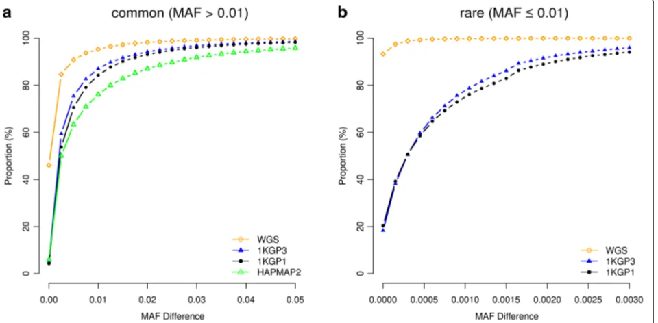
MAF differences < 0.003) (Fig. 1), suggesting that the as-sociation signal at a rare causal variant is highly unlikely to be mapped to a common variant in GWAS using ei-ther WGS or imputed data and vice versa. We then quantified the proportion of GWAS hits within a given physical distance from the corresponding causal variants (Fig. 2). For common variants, the majority of the top associated variants in GWAS were in < 100 Kbp distance from the causal variants, from 94.8% for GWAS using HapMap2-imputed data to 98.3% using WGS data (Fig. 2a), in line with the result from a recent study that most of the candidate causal variants (inferred from a fine mapping analysis with epigenetic data) are within 100 Kbp of the GWAS top hits [15]. It should be noted that the result for WGS data was not 100% because the causal variant was not always the top associated variant in GWAS (Fig. 3) due to the complicated linkage dis-equilibrium (LD) structure between genetic variants in close proximity and the sampling variation in the test-statistics (see Additional file 1: Figure S5a for a simple example). The results also suggest that for published GWAS using imputed data from HapMap2 or 1KGP, at least 80% of the top associated GWAS variants are within 33.5 Kbp distance of the causal variants. The mapping precision for 1KGP1-based imputation was higher than that for HapMap2-based imputation but the difference was not large (27.6 Kbp versus 33.5 Kbp at 80%). The difference between 1KGP1 and 1KGP3 was subtle (27.6 Kbp versus 25.1 Kbp at 80%). All the results suggest that the strategy of SNP array-based genotyping
with subsequent imputation has already provided a high mapping resolution that is comparable with that using WGS, consistent with the conclusion from our previous study [10] that WGS is not a cost-effective approach to map common variants for complex traits.
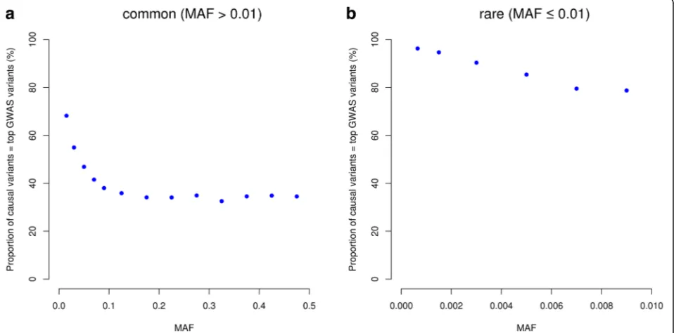
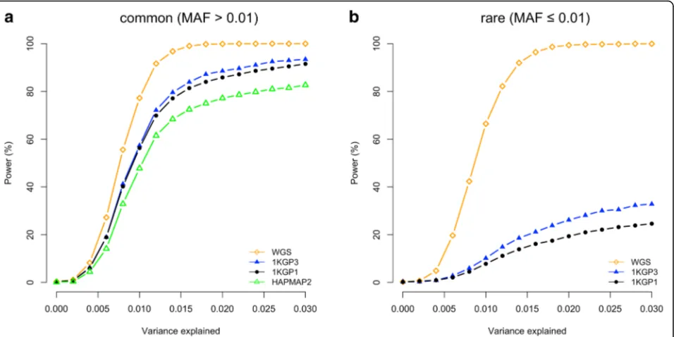
For rare variants, however, the results were different. The difference between WGS and 1KGP-impution was very large. There were 94.2% of the GWAS hits within a dis-tance of 5 Kbp of the causal variants for WGS but only 36.6% for 1KGP3-based imputation. This is because the number of variants in high LD with a rare variant was much smaller than that for a common variant (Additional file 1: Figure S6) and thus it is more likely for a rare causal variant being detected as the top signal in WGS data than a common variant. It is shown in Fig. 3 that 98% of causal variants were detected as the top signals in GWAS for very rare variants (0.0003 < MAF < 0.001) and the proportion decreased to ~30–40% for very common variants (MAF > 0.1). Approximately 68.1% of the GWAS hits were within a distance of 100 Kbp of the causal variants for 1KGP3-based imputation (Fig. 2b), which was much smaller than that (98.2%) for WGS (Fig. 2b). These results suggest that map-ping precision of GWAS using imputed data for rare vari-ants is much lower than that for common varivari-ants (Fig. 2), and these results are not driven by sampling variation in LDr2(Additional file 1: Figure S7). Moreover, the statistical power of detection for rare variants using imputed data was also much lower than that for common variants (Fig. 4) be-cause rare variants were less well imputed than common variants [12, 16]. There were a substantial proportion of
[image:3.595.62.542.459.695.2]causal variants, especially rare causal variants, which were mapped to variants in more than 100 Kb distance even at an extremely stringent P value threshold (i.e. P< 5e-11) (Additional file 1: Figure S8). This is because in comparison with common variants, rare variants have fewer LD proxies
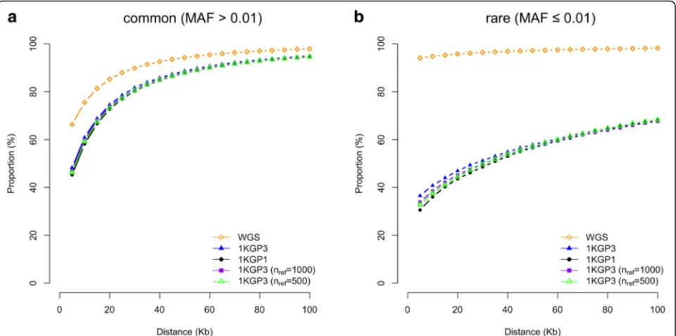
within 100 Kb distance (Additional file 1: Figure S6), less likely to be present in the reference panel (2.2% of the com-mon variants and 50.4% of the rare variants in UK10K-WGS are absent in 1KGP3), and less well imputed even if they are present in the reference panel [12, 16], their Fig. 2Mapping precision of GWAS based on different genotyping strategies. Results are from 50,000 simulations for causal common (a) and rare (b) variants, respectively, based on the UK10K-WGS data. Shown on they-axis is the proportion of causal variants that were mapped to variants within a certain distance as specified on thex-axis
[image:4.595.59.538.88.327.2] [image:4.595.60.539.467.704.2]association signals are therefore more likely to be mapped to distant variants due to the complicated LD structure of genome as illustrated in Additional file 1: Figure S9. Taken all together, our results demonstrate the benefit of using WGS as a strategy for detecting and fine-mapping rare vari-ants simultaneously. For real data, ignoring cost consider-ations, the advantage of using WGS in GWAS depends on the proportion of heritability for the trait or disease that is attributable to rare variants [10, 17]. In addition, the sample size of WGS data needs to be very large because the statis-tical power of GWAS to detect a variant is determined by the non-centrality parameter (NCP) of theχ2test-statistic, i.e. NCP =nq2/(1 –q2), wheren is the sample size of the GWAS data,q2= 2f(1–f)b2withbbeing the effect size per allele andf being the allele frequency. For rare variants, if
q2
is small, NCP≈nq2≈2nfb2.
We observed little difference in mapping precision between the analyses based on data imputed to 1KGP1 and 1KGP3 (Fig. 2) despite that the sample size of 1KGP3 (nref= 2504) is ~2.5 times larger than that of 1KGP1 (nref
= 1092). There was an apparent, although also not large, difference in power between 1KGP1 and 1KGP3 (Fig. 4). We then investigated the mapping precision as a function ofnref by re-running the imputation to a random subset
of individuals from 1KGP3 (nref= 500 and 1000). The
add-itional imputation analyses showed consistent results, i.e. power slightly increased withnrefin particular for rare
var-iants (Additional file 1: Figure S10) whereas mapping pre-cision was almost independent from nref for either
common or rare variants (Fig. 5). To further investigate
the influence of nrefon the mapping precision of GWAS
using imputed data, we performed additional analyses using genotyped data from a larger GWAS cohort (i.e. the Health Retirement Study [HRS] [18]) and imputed the ge-notyped data to a much larger reference panel (i.e. HRC). There were 8479 unrelated individuals in HRS genotyped on ~1.7 million SNPs (1,451,882 common and 243,548 rare) after QC [10]. We left out 50,000 common and 50,000 rare SNPs as a pool to sample causal variants for simulations and imputed the genotypes of the remaining SNPs to 1KGP3 and HRC. We performed 50,000 simula-tions for common and rare variants, respectively. In each simulation replicate, we randomly sampled a variant from the causal variant pool (50,000 common and 50,000 rare SNPs) and simulated a quantitative phenotype using the method described above withq2= 0.87% (NCP = 74, simi-lar as that in the UK10K simulation). We then performed GWAS analyses of the simulated phenotype using the 1KGP3- and HRC-imputed data. We observed little differ-ence in mapping precision between the results using 1KGP3- and HRC-imputed data (Additional file 1: Figure S11), consistent with our observations above that mapping precision of GWAS using imputed data was almost inde-pendent of nref. We further performed simulations in a
[image:5.595.61.539.88.327.2]imputed UK10K data (Additional file 1: Figure S11 and Fig. 2). This is because almost all the rare causal variants in HRS were available in 1KGP3 (only 5.9% were not avail-able) whereas more than a half (50.2%) of the rare causal variants in UK10K were not available in 1KGP3. To con-firm this, we re-calculated the mapping precision in the 1KGP3-imputed UK10K data focusing only on the causal variants that were available in 1KPG3. The result was al-most identical to that observed in the HRS data imputed to either 1KGP3 or HRC (Additional file 1: Figure S12). These observations suggest that the low mapping pre-cision for rare variants in GWAS using imputed data is mainly due to a large proportion of rare causal var-iants that are not available in the reference. Taken to-gether, our results seem to suggest that the mapping precision of GWAS using imputed data increases with the variant-coverage of the imputation reference but is almost independent of the sample size of the refer-ence (although these two factors are intertwined). In addition, we observed that having the causal variants in the reference not only improved mapping precision (Fig. 2 and Additional file 1: Figure S13) but also in-creased statistical power (Fig. 4 and Additional file 1: Figure S14). The difference in power between the two sets of variants (available versus not available in the reference) can be quantified as the loss of power at-tributable to imputation accuracies (the variance ex-plained by GWAS hit qGWAS2 =q2Rimp2 , where Rimp2 is the squared imputation accuracy) and imperfect
tagging (qGWAS2 =q2R2impr2, where r2 is LD r2 between GWAS hit and causal variant).
We next investigated the influence of GWAS sample size (n) on mapping precision. We demonstrated by sim-ulations under a simple scenario that the probability of causal variant being detected as the top signal in GWAS with sequencing data depends on NCP (Additional file 1: Figure S5), which is a function of both q2 and n(see the equations above). This explains why the mapping precision slightly decreased with decreasednorq2in ei-ther WGS or 1KGP-imputed data (Additional file 1: Fig-ure S15). In our simulations, in order to obtain sufficient power to detect the simulated genetic effects at a genome-wide significance level (e.g. P< 5e-8) using a relatively small sample size (n= 3642 unrelated individ-uals), we simulated causal variants of relatively large ef-fect (q2= 2% in most of the analyses). Given n= 3642 andq2= 2%, the NCP at any of the simulated causal var-iants was 74.3, which is approximately equivalent to a setting withn= 250,000 andq2= 0.03% (note that the es-timated mean q2 of the published 679 height SNPs is ~0.03% from the GIANT meta-analysis [19] with n= ~250,000), suggesting that the conclusions we drew from our simulations can be applied in general to studies at the current scale (n= 100,000s) and that mapping preci-sion at the known loci will be improved in the future with larger sample sizes. The conclusion has further been supported by evidence from simulations in the HRS dataset with a wider range of sample sizes and Fig. 5Mapping precision of GWAS based on imputations with different sample sizes of the reference panel. Shown are results from 50,000 simulations for common (a) and rare (b) variants, respectively. 1KGP3 (nref= 1000) and 1KGP3 (nref= 500): SNP array data imputed to a random
[image:6.595.59.539.88.327.2]NCP (Additional file 1: Figure S16). In addition, we in-vestigated the impact of P value threshold on mapping precision. We found that mapping precision of GWAS using sequenced or imputed common variants or se-quenced rare variants did not change with P value threshold (Additional file 1: Figure S8). However, map-ping precision of GWAS using rare imputed variants at
P< 5e-11 was substantially larger than that at P< 5e-8. This is because distant tagging variants were dispropor-tionately more likely to be removed by the stringent thresholdP< 5e-11 (Additional file 1: Figure S17).
Discussion and conclusions
We have shown above results from simulations where the causal variants were randomly sampled from the se-quence variants. In reality, however, it might not be the case. It has been suggested in previous studies that trait-associated or disease-trait-associated variants are not ran-domly distributed but enriched in some functional
cat-egories of the genome such as the DNase I
hypersensitive sites (DHSs) [20, 21]. We therefore per-formed simulations by sampling causal variants from DHSs where the SNPs are in lower LD [10, 20]. The re-sults were almost exactly the same as those presented above (Additional file 1: Figure S18), suggesting mapping precision is almost independent of the distribution of the causal variants in the genome. All the imputation analyses presented above are based on Illumina CoreEx-ome array. We chose the Illumina CoreExCoreEx-ome array be-cause it is the most cost-effective SNP array with respect to capturing genetic variation among all the SNP arrays investigated in a previous study [10] and because the number of SNPs on an Illumina CoreExome array (312,264 SNPs after QC) is relatively small (Additional file 1: Table S4) so that the mapping precision quantified based on this array is likely to be conservative and can therefore be used as a benchmark to guide the design of fine-mapping studies. In a meta-analysis of GWAS, how-ever, data from different participating cohorts are usually genotyped on different types of SNP genotyping arrays. We then repeated the analysis for four additional types of SNP arrays (i.e. Affymetrix 6, Affymetrix Axiom Genome-Wide EUR Array [22], Illumina OmniExpress, and Illumina Omni2.5). The number of variants in each array is listed in Additional file 1: Table S4. The results were all very similar except that Illumina Omni2.5 per-formed slightly better than the other types of arrays for both common and rare variants (Additional file 1: Figure S19), which is likely because of its denser SNP coverage. Given these results, if data from all participating cohorts are imputed to the same imputation reference (e.g. 1KGP), heterogeneity in mapping precision across co-horts is likely to be small. These results also imply that to design a SNP-array based GWAS study with a fixed
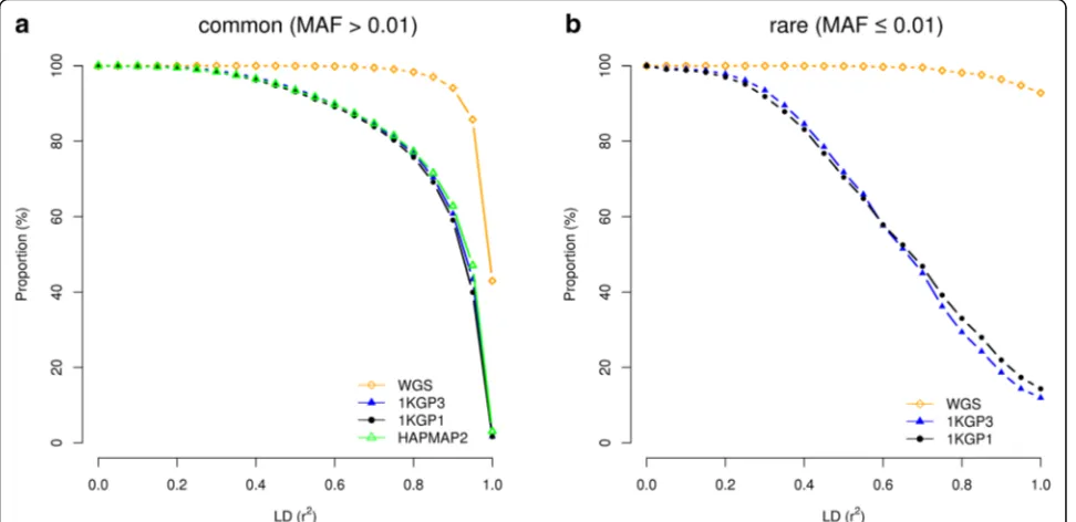
budget, the most cost-effective design is to choose the cheapest SNP array with genome-wide coverage and maximize experimental sample size, in line with the con-clusion drawn from our previous study [10]. In all the analyses above, we used physical distance to assess the mapping precision. In practice, however, it is sometimes also useful to know the distribution of LD between GWAS top hits and causal variants. To this end, we quantified the mapping precision by the squared LD cor-relation (r2) between causal variants and GWAS hits (Fig. 6). Interestingly, for common variants in GWAS using imputed data, at least 77.3% of the association sig-nals were mapped to SNPs in LDr2> 0.8 with the causal variants. We further developed an online tool (gwasMP) [26] for querying our results with different thresholds of physical distance and/or LD (http://cnsgenomics.com/ shiny/gwasMP).
There are certainly more complicated scenarios (e.g. multiple common and rare causal variants in a very small genomic region) that have not been investigated in our simulations. However, these scenarios are unlikely to be the norm and thus are unlikely to bias our results substantially. With limited sample size of the WGS data (n= 3642) we were only able to quantify the mapping precision for rare variants with MAF down to 0.0003. For rarer variants, larger population-based cohorts with WGS data are required. Our conclusions were drawn from simulations based on modern SNP arrays with 100,000s SNPs, which cannot be applied to studies based on low-dense markers. It should also be noted that all our results are from analyses in European populations, these results need to be applied with caution to non-European populations (e.g. Asian and African popula-tions), given the substantial differences in LD structure between Europeans and non-Europeans. We also did not simulate a case-control design because the sample size of UK10K-WGS data is not large enough to simulate an ascertained case-control study of sufficiently large sam-ple size for a disease of reasonable prevalence. However, the general conclusions about mapping precision should be applicable to case-control studies because mapping precision is essentially determined by the strength of the association signal, LD structure and imputation preci-sion, rather than the scale of the phenotype. Neverthe-less, this needs to be confirmed in the future by simulations of case-control design using large WGS datasets.
at least 80% of the top associated common variants identi-fied from published GWAS are within 33.5 Kbp distance of the causal variants, and mapping precision at these loci can be improved in the future with larger sample sizes. For im-puted data, the differences in mapping precision between different SNP genotyping arrays were trivial. Mapping pre-cision of GWAS using imputed data increased with variant-coverage of the reference panel but was almost independent of sample size of the reference. These two factors, however, are not independent. WGS with increasingly large sample sizes and improved sequencing technology will provide more genetic variants [14] in the reference panels in a fore-seeable near future, which will certainly improve the map-ping precision of GWAS using data imputed from these large reference panels. For rare variants, the mapping preci-sion of GWAS based on WGS data was extremely high, much higher than that based on imputation. This implies the potential of using WGS as an efficient strategy for de-tecting and fine-mapping rare variants at the same time. All these findings provide an important benchmark to inform the design and development of fine-mapping experiments and technologies in the future to identify causal variants at the GWAS loci.
Methods
Simulation based on WGS data
We used WGS data from the UK10K project
(UK10K-WGS) [7] for simulations. The data consist of 3781 individuals and ~45.5 million genetic variants.
We excluded SNPs with missingness > 0.05, Hardy-Weinberg equilibrium test P value < 1 × 10⁻⁶, or minor allele count (MAC) < 3 (equivalent to MAF < 0.0003) using PLINK [23]. We chose a MAC old of 3 because we sought to choose a MAF thresh-old as low as possible to make general inferences about rare-variant associations but excluded single-tons and doublesingle-tons as they are more subject to se-quencing errors. We further removed individuals with genotype missingness rate > 0.05 and one of each pair of individuals with estimated genetic relatedness > 0.05. The genetic relatedness was estimated from GCTA [24] using all the common SNPs on HapMap phase 3 (HapMap3). A total of 3642 unrelated indi-viduals and 17.6 million variants were retained for
analysis. We randomly sampled a variant from
UK10K-WGS as causal variant and generated the phenotype based on the model y=g+e, with g=wu and w¼ðx−2fÞ=p2ffiffiffiffiffiffiffiffiffiffiffiffiffiffiffiffifð1−fÞ, where x is the indicator variable for the genotypes of causal variant (coded as 0, 1or 2), f is the frequency of the coded allele, and u is the effect size per standardized genotype sampled from N(0, 1). The residual e was generated from N(0,
var(g)(1/q2−1)) with q2 being the proportion of vari-ance in phenotype explained by the causal variant. We performed a GWAS analysis for the simulated trait using the variants from different genotyping strategies (see below for details about the genotyping Fig. 6Mapping precision of GWAS as measured by the squared LD correlations between causal variants and GWAS top SNPs based on different genotyping strategies. Results are from 50,000 simulations for causal common (a) and rare (b) variants, respectively, based on the UK10K-WGS data. Shown on they-axis is the proportion of causal variants that were mapped to variants with LDr2smaller than a certain threshold as
[image:8.595.57.543.89.325.2]strategies) and selected the top associated variant that passed a genome-wide significance level (e.g. P value < 5e-8). We repeated the simulation to quantify the power at different levels of q2 (from 0 to 3% at 0.2% intervals; 5000 replicates at each q2 level). Note that the simulations at q2= 0 quantify the false positive rate. We then repeated the simulation 50,000 times at q2= 2% to quantify the mapping precision (i.e. physical distance between the top associated variant identified in GWAS analysis and the simulated causal variant) for common and rare variants, respectively. We further repeated analysis to quantify the mapping precision by sampling causal variants from the DNase I hypersensitive sites (DHSs) to mimic the observa-tion that genetic variants associated with complex traits are enriched in DHSs [10, 20].
Imputation of SNP-array data to multiple reference panels We performed simulations to quantify the mapping preci-sion using three different genotyping strategies, i.e. WGS, SNP-array data imputed to HapMap 2 reference panel (HapMap2) [8], and SNP-array data imputed to 1000 Gen-ome project reference panels (1KGP) [9]. The method to mimic the strategy of SNP-array genotyping followed by imputation is described in Yang et al. [10]. That is, we ex-tracted SNPs that are on Illumina CoreExome arrays from the UK10K-WGS data, phased genotypes using SHAPEIT [25], and imputed the data to HapMap2, 1KGP phase 1 (1KGP1), and 1KGP phase 3 (1KGP3) by IMPUTE2 [11]. To investigate the power and mapping precision as a func-tion of sample size of the imputafunc-tion reference, we further performed the imputation analyses using a subset of indi-viduals randomly sampled from 1KGP3 (n= 500 and 1000) as the reference panel.
To investigate the influence of reference sample size on the mapping precision of GWAS using imputed data, we performed additional analyses using genotyped data from HRS and imputed the genotyped data to HRC. There were 8479 unrelated individuals in HRS genotyped on ~1.7 mil-lion SNPs (1,451,882 common and 243,548 rare) after QC. We left out 50,000 common and 50,000 rare SNPs as a pool to sample causal variants for simulations and imputed the genotypes of the remaining SNPs to the 1KGP3 and HRC reference panel [12] respectively using Sanger imputation server (https://imputation.sanger.ac.uk/).
Additional files
Additional file 1:This PDF file containsFigures S1–S19, Tables S1–S4,
andText S1. (PDF 5824 kb)
Funding
This research was supported by the Australian Research Council
(DP160101343), the Australian National Health and Medical Research Council
(1078037, 1107258 and 1113400), and the Sylvia & Charles Viertel Charitable Foundation (Senior Medical Research Fellowship).
Availability of data and materials
This study makes use of data from dbGaP (accessions: phs000428.v1.p1) and EGA (accessions: EGAS00001000108 and EGAS00001000090) (see Additional file 1: Text S1 for a full list of acknowledgements to these data sets). The source code of gwasMP is available at a DOI-assigning repository zenodo (https://doi.org/10.5281/zenodo.556343) and at GitHub (https://github.com/ jianyangqt/gwasMP/) under GNU General Public License v3.0.
Authors’contributions
JY, YW and PMV conceived and designed the experiments. YW performed the statistical analyses. ZZ, YW and JY developed the online tool. YW and JY wrote the paper. All authors read and approved the final manuscript.
Competing interests
The authors declare that they have no competing interests.
Ethics approval and consent to participate
Not applicable.
Publisher’s Note
Springer Nature remains neutral with regard to jurisdictional claims in published maps and institutional affiliations.
Author details
1
Institute for Molecular Bioscience, The University of Queensland, Brisbane, QLD 4072, Australia.2Queensland Brain Institute, The University of
Queensland, Brisbane, QLD 4072, Australia.3The Eye Hospital, School of Ophthalmology & Optometry, Wenzhou Medical University, Wenzhou, Zhejiang 325027, China.
Received: 28 December 2016 Accepted: 20 April 2017
References
1. Welter D, MacArthur J, Morales J, Burdett T, Hall P, Junkins H, et al. The NHGRI GWAS Catalog, a curated resource of SNP-trait associations. Nucleic Acids Res. 2014;42:1001–6.
2. Smemo S, Tena JJ, Kim KH, Gamazon ER, Sakabe NJ, Gomez-Marin C, et al. Obesity-associated variants within FTO form long-range functional connections with IRX3. Nature. 2014;507:371–5.
3. Claussnitzer M, Dankel SN, Kim K-H, Quon G, Meuleman W, Haugen C, et al. FTO obesity variant circuitry and adipocyte browning in humans. N Engl J Med. 2015;373:895–907.
4. Sekar A, Bialas AR, de Rivera H, Davis A, Hammond TR, Kamitaki N, et al. Schizophrenia risk from complex variation of complement component 4. Nature. 2016;530:177–83.
5. Musunuru K, Strong A, Frank-Kamenetsky M, Lee NE, Ahfeldt T, Sachs KV, et al. From noncoding variant to phenotype via SORT1 at the 1p13 cholesterol locus. Nature. 2010;466:714–9.
6. Ulirsch JC, Nandakumar SK, Wang L, Giani FC, Zhang X, Rogov P, et al. Systematic functional dissection of common genetic variation affecting red blood cell traits. Cell. 2016;165:1530–45.
7. UK10K Consortium, Walter K, Min JL, Huang J, Crooks L, Memari Y, et al. The UK10K project identifies rare variants in health and disease. Nature. 2015; 526:82–90.
8. The International HapMap Consortium, Gibbs RA, Belmont JW, Boudreau A, Leal SM, Hardenbol P, et al. A haplotype map of the human genome. Nature. 2005;437:1299–320.
9. 1000 Genomes Project Consortium, Abecasis GR, Altshuler D, Auton A, Brooks LD, Durbin RM, et al. A map of human genome variation from population-scale sequencing. Nature. 2010;467:1061–73.
10. Yang J, Bakshi A, Zhu Z, Hemani G, Vinkhuyzen AAE, Lee SH, et al. Genetic variance estimation with imputed variants finds negligible missing heritability for human height and body mass index. Nat Genet. 2015;47:1114–20. 11. Howie BN, Donnelly P, Marchini J. A flexible and accurate genotype
12. McCarthy S, Das S, Kretzschmar W, Delaneau O, Wood AR, Teumer A, et al. A reference panel of 64,976 haplotypes for genotype imputation. Nat Genet. 2016;48:1279–83.
13. Fadista J, Manning AK, Florez JC, Groop L. The (in)famous GWAS P-value threshold revisited and updated for low-frequency variants. Eur J Hum Genet. 2016;24:1202–5.
14. Telenti A, Pierce LC, Biggs WH, di Iulio J, Wong EH, Fabani MM, et al. Deep sequencing of 10,000 human genomes. Proc Natl Acad Sci U S A. 2016;113: 11901–6.
15. Farh KK, Marson A, Zhu J, Kleinewietfeld M, Housley WJ, Beik S, et al. Genetic and epigenetic fine mapping of causal autoimmune disease variants. Nature. 2015;518:337–43.
16. Huang J, Howie B, McCarthy S, Memari Y, Walter K, Min JL, et al. Improved imputation of low-frequency and rare variants using the UK10K haplotype reference panel. Nat Commun. 2015;6:8111.
17. Liu Dajiang J, Leal SM. Estimating genetic effects and quantifying missing heritability explained by identified rare-variant associations. Am J Hum Genet. 2012;91:585–96.
18. Sonnega A, Faul JD, Ofstedal MB, Langa KM, Phillips JW, Weir DR. Cohort Profile: the Health and Retirement Study (HRS). Int J Epidemiol. 2014;43:576–85. 19. Wood AR, Esko T, Yang J, Vedantam S, Pers TH, Gustafsson S, et al. Defining
the role of common variation in the genomic and biological architecture of adult human height. Nat Genet. 2014;46:1173–86.
20. Gusev A, Lee SH, Trynka G, Finucane H, Vilhjalmsson BJ, Xu H, et al. Partitioning heritability of regulatory and cell-type-specific variants across 11 common diseases. Am J Hum Genet. 2014;95:535–52.
21. Finucane HK, Bulik-Sullivan B, Gusev A, Trynka G, Reshef Y, Loh P-R, et al. Partitioning heritability by functional annotation using genome-wide association summary statistics. Nat Genet. 2015;47:1228–35.
22. Hoffmann TJ, Kvale MN, Hesselson SE, Zhan Y, Aquino C, Cao Y, et al. Next generation genome-wide association tool: design and coverage of a high-throughput European-optimized SNP array. Genomics. 2011;98:79–89. 23. Purcell S, Neale B, Todd-Brown K, Thomas L, Ferreira MA, Bender D, et al.
PLINK: a tool set for whole-genome association and population-based linkage analyses. Am J Hum Genet. 2007;81:559–75.
24. Yang J, Lee SH, Goddard ME, Visscher PM. GCTA: A tool for genome-wide complex trait analysis. Am J Hum Genet. 2011;88:76–82.
25. O’Connell J, Gurdasani D, Delaneau O, Pirastu N, Ulivi S, Cocca M, et al. A general approach for haplotype phasing across the full spectrum of relatedness. PLoS Genet. 2014;10:e1004234.
26 gwasMP: quantifying the mapping precision of GWAS. doi:10.5281/zenodo. 556343.
• We accept pre-submission inquiries
• Our selector tool helps you to find the most relevant journal • We provide round the clock customer support
• Convenient online submission • Thorough peer review
• Inclusion in PubMed and all major indexing services • Maximum visibility for your research
Submit your manuscript at www.biomedcentral.com/submit