Rewriting Schemes for Flash Memory

Thesis by

Eyal En Gad

In Partial Fulfillment of the Requirements for the Degree of

Doctor of Philosophy

California Institute of Technology Pasadena, California

2015

c

2015

Acknowledgments

I would like to start by acknowledging my advisor Jehoshua (Shuki) Bruck, for his enormous contributions to this thesis and to my professional and personal development during my time at Caltech. Shuki’s advices about problem selection, motivation, solutions, and presentation led me to enjoy my work greatly and to take pride in my results. He also taught me how to be always optimistic and kind, and to enjoy fruitful collaborations. I feel very lucky and grateful for having the opportunity to study under him.

During my graduate studies I was lucky to collaborate and learn from many other won-derful researchers. Moshe Schwartz introduced me to the beauty and utility of combinatorial coding theory, and taught me many useful ways to present research ideas. His sharp mind and kind attitude were very inspiring for me. Michael Langberg taught me many concepts in combinatorics and information theory with a very thorough approach. I also learned a lot from him about how to explain research results in an interesting and clear way, and how to always be kind and pleasant with everyone. Andrew Jiang introduced me to wonderful ideas about coding in flash memory. His energy and excitement are contagious and make every discussion with him very joyful. Joerg Kliewer introduced me to many concepts in modern coding theory, and is always exited to explore new research directions. The discussions with him gave me many exiting ideas and new perspectives.

me towards research, and for his constant smile that kept the atmosphere in lab always cheerful. I am also thankful for many challenging racquetball matches with him. Another great collaborator and lab-mate is Wentao Huang, with whom I worked in the last part of my studies. I am thankful to Wentao’s dedication and innovative thinking that made this work very exiting.

I am also thankful to the many other lab members that I did not have the chance to collaborate with: Daniel Wilhelm, Hongchao Zhou, Zhiying Wang, David Lee, Itzhak Tamo, Lulu Qian, Farzad Farnoud, and Siddharth Jain.

I would like to thank Robert Mateescu, who hosted me in an internship at HGST. I had a great time during the three months I spent at the Storage Architecture group. I am very grateful to my collaborators at HGST - Filip Blagojevic, Cyril Guyot and Zvonimir Bandic - and to the other friendly people at the research group, including Dejan Vucinic, Qingbo Wang, Luiz Franca-Neto, and Jorge Campello.

I would like to thank my thesis committee: Michelle Effros, Babak Hassibi and P. P. Vaidyanathan. Their illuminating questions and comments provided me with different points of view and new ways of thinking.

I am very thankful for the remote support of my family and friends in Israel. My mother Orna, my stepfather Uri, my brother Oded and my sister Neta. Your love and support was an indispensable ingredient of the success and joy I had in my doctoral studies.

Abstract

Flash memory is a leading storage media with excellent features such as random access and high storage density. However, it also faces significant reliability and endurance challenges. In flash memory, the charge level in the cells can be easily increased, but removing charge requires an expensive erasure operation. In this thesis we study rewriting schemes that enable the data stored in a set of cells to be rewritten by only increasing the charge level in the cells. We consider two types of modulation scheme; a convectional modulation based on the absolute levels of the cells, and a recently-proposed scheme based on the relative cell levels, called rank modulation. The contributions of this thesis to the study of rewriting schemes for rank modulation include the following: we

• propose a new method of rewriting in rank modulation, beyond the previously proposed method of “push-to-the-top”;

• study the limits of rewriting with the newly proposed method, and derive a tight upper bound of 1 bit per cell;

• extend the rank-modulation scheme to support rankings with repetitions, in order to improve the storage density;

• derive a tight upper bound of 2 bits per cell for rewriting in rank modulation with repetitions;

The next part of this thesis studies rewriting schemes for a conventional absolute-levels modulation. The considered model is called “write-once memory” (WOM). We focus on WOM schemes that achieve the capacity of the model. In recent years several capacity-achieving WOM schemes were proposed, based on polar codes and randomness extractors. The contributions of this thesis to the study of WOM scheme include the following: we

• propose a new capacity-achieving WOM scheme based on sparse-graph codes, and show its attractive properties for practical implementation;

• improve the design of polar WOM schemes to remove the reliance on shared randomness and include an error-correction capability.

Contents

Acknowledgments iv

Abstract vi

I

Introduction

1

1 Rewriting in Flash Memory 2

1.1 Rank Modulation . . . 3 1.2 Write-Once Memory . . . 6 1.3 Local Rank Modulation . . . 8

II

Rewriting with Rank Modulation

10

2 Model and Limits of Rewriting Schemes 11

2.1 Modifications to the Rank-Modulation Scheme . . . 11 2.2 Definition and Limits of Rank-Modulation Rewriting Codes . . . 16 2.3 Proof of the Cost Function . . . 22

3 Efficient Rewriting Schemes 25

3.4 Summary . . . 53

3.5 Capacity Proofs . . . 54

III

Write-Once Memory

57

4.2 Rewriting with Message Passing . . . 61

4.3 Error-Correcting Rewriting Codes . . . 66

4.4 Summary . . . 71

5 Rewriting with Polar Codes 72 5.1 Relation to Previous Work . . . 72

5.2 Asymmetric Point-to-Point Channels . . . 74

5.3 Channels with Non-Causal Encoder State Information . . . 82

5.4 Summary . . . 93

5.5 Capacity Proofs . . . 94

5.6 Proof of Theorem 5.7 . . . 100

IV

Local Rank Modulation

109

6.2 Constant-Weight Gray Codes for (1,2, n)-LRM . . . 118

6.3 Gray Codes for (s, t, n)-LRM . . . 124

6.4 Summary . . . 139

List of Figures

3.1 Iteration i of the encoding algorithm, where 1_≤i_≤q₋r₋1. . . 34

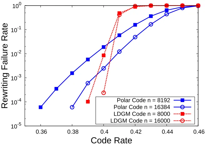
4.1 Rewriting failure rates of polar and LDGM WOM codes. . . 65

4.2 Encoding performance of the codes in Table 4.1. . . 68

5.1 Encoding the vector u[n]. . . 77

5.2 Example 5.1: A binary noisy WOM model. . . 85

5.3 Example 5.2: A binary WOM with writing noise. . . 86

5.4 Encoding the vector u[n] in Construction 5.2. . . 88

5.5 The chaining construction . . . 91

6.1 Demodulating a (3,5,12)-locally rank-modulated signal. . . 111

List of Tables

1.1 WOM-Code Example . . . 3

4.1 Error-correcting Rewriting Codes from Conjugate Pairs . . . 68

4.2 Error-correcting rewriting codes of length _≈8200. . . 71

6.1 A cyclic optimal (1,2,5; 2)-LRMGC . . . 117

Part I

Chapter 1

Rewriting in Flash Memory

This thesis deals with coding schemes for data storage in flash memory. Flash memory is a leading storage media with many excellent features such as random access and high storage density. However, it also faces significant reliability and endurance challenges. Flash memory contains floating gate cells. The cells are electrically charged with electrons and can represent multiple levels according to the number of electrons they contain. The most conspicuous property of flash-storage technology is its inherent asymmetry between cell programming and cell erasing. While it is fast and simple to increase a cell level, reducing its level requires a long and cumbersome operation of first erasing its entire containing block (∼ 106_cells)

and only then programming the cells [8]. Such block erasures are not only time consuming, but also degrade the lifetime of the memory. A typical block can generally tolerate at most 104₋₁₀5 _erasures.

To reduce the amount of block erasures, the focus of this thesis is on schemes for the

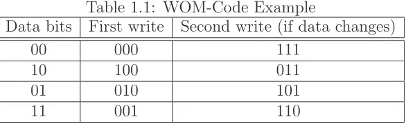
Table 1.1: WOM-Code Example

Data bits First write Second write (if data changes)

00 000 111

10 100 011

01 010 101

11 001 110

memories.

The first example of a rewriting scheme was given by Rivest and Shamir in 1982 [69]. This example considers a rewriting model called write-once memory (WOM), in which the memory cells take binary values, and can only change for 0 to 1. The example is a simple WOM code that enables the recording of two bits of information in three memory cells twice. The encoding and decoding rules for this WOM-code are described in a tabular form in Table 1.1. It is easy to verify that after the first 2-bit data vector is encoded into a 3-bit codeword, if the second 2-bit data vector is different from the first, the 3-bit codeword into which it is encoded does not change any code bit 1 into a code bit 0, ensuring that it can be recorded in the write-once medium.

WOM codes with more cells and more data bits were studied extensively in recent years, since the emergence of the flash memory application. In this thesis we make several contri-bution to the study of WOM codes. In addition to WOM, the thesis also studies rewriting in a different data-representation scheme, called rank modulation. We turn our attention now to describe the rewriting setting in rank modulation.

1.1

Rank Modulation

cell 1 and then cell 2 with the lowest level. Each ranking can represent a distinct information message, and so the 3 cells in this example store together log₂6 bits. It was suggested in [45] that the rank-modulation scheme speeds up data writing by eliminating the over-shooting problem in flash memories. In addition, it also increases the data retention by mitigating the effect of charge leakage.

Rank-modulation rewriting codes were proposed in [45, Section IV], with respect to a rewriting method called “push-to-the-top”. In this rewriting method, the charge level of a single cell is pushed up to be higher than that of any other cell in the ranking. In other words, a push-to-the-top operation changes the rank of a single cell to be the highest. A rewriting operation involves a sequence of push-to-the-top operations that transforms the cell ranking to represent a desired updated data. The cells, however, have an upper limit on their possible charge levels. Therefore, after a certain number of rewriting operations, the user must resort to the expensive erasure operation in order to continue updating the memory. The concept of rewriting codes was proposed in order to control the trade-off between the number of data updates and the amount of data stored in each update. Note that the number of performed push-to-the-top operations determines when an expensive block erasure is required. However, the number of rewriting operations itself does not affect the triggering of the block erasure. Therefore, rewriting operations that require fewer push-to-the-top operations can be seen as cheaper, and are therefore more desirable. Nevertheless, limiting the memory to cheap rewriting operations would reduce the number of potential rankings to write, and therefore would reduce the amount of information that could be stored. We refer to the number of push-to-the-top operations in a given rewriting operation as thecost of rewriting. The study in [45, Section IV] considers rewriting codes with a constrained rewriting cost.

desired cell, instead of only above the level of the top cell. We justify both modifications and devise an appropriate notion of rewriting cost. Specifically, we define the cost to be the difference between the charge level of the highest cell, after the writing operation, to the charge level of the highest cell before the rewriting operation. We suggest and explain why the new cost function compares fairly to that of the push-to-the-top model. We then go on to study rewriting codes in the modified framework.

We measure the storage rate of rewriting codes by the ratio between the number of stored information bits in each write, to the number of cells in the ranking. We study the case in which the number of cells is large (and asymptotically growing), while the cost constraint is a constant, as this case appears to be fairly relevant for practical applications. In the model of push-to-the-top rewriting which was studied in [45, Section IV], the storage rate vanishes when the number of cells grows. Our first interesting result is that the asymptotic storage rate in our modified framework converges into a positive value (that depends on the cost constraint). Specifically, using rankings without repetitions, i.e. the original rank modulation scheme with the modified rewriting operation, and the minimal cost constraint of a single unit, the best storage rate converges to a value of 1 bit per cell. Moreover, when ranking with repetitions is allowed, the best storage rate with a minimal cost constraint converges to a value of 2 bits per cell.

1.2

Write-Once Memory

In Part III of this thesis we propose two new constructions of WOM codes. These construc-tions can be used with an absolute-level modulation, or with the rank-modulation rewriting schemes proposed in Part II.

The constructions proposed in this thesis are based on sparse-graph codes and on polar codes. Sparse-graph WOM codes are introduced in this thesis, while polar WOM codes were discovered earlier (in [7]), and this thesis contributes to their study. Many other types of WOM codes were proposed in the literature, including [21, 25, 43, 44, 86, 88, 91].

An important feature of both WOM schemes proposed in this thesis is that they achieve the capacity of the WOM model (given in [36]). The sparse-graph WOM codes achieve the capacity of the WOM for two writes, while the polar WOM codes achieve the capacity for any number of writes. In both schemes we also propose methods to integrate the WOM codes with error-correcting codes.

1.2.1

Sparse-Graph WOM codes

information embedding, which shares some similarity with our model.

Moreover, the proposed construction is extended with error correction. We use conjugate code pairs studied in the context of quantum error correction [35]. As an example, we construct LDGM WOM codes whose codewords also belong to BCH codes. Therefore, our codes allow to use any decoding algorithm of BCH codes. The latter have been implemented in most commercial flash memory controllers. We also present two additional approaches to add error correction, and compare their performance.

1.2.2

Polar WOM codes

Polar WOM codes were introduced in [7]. The construction is based on polar lossy source codes of Korada and Urbanke [50], which are based on the polar channel codes of Arikan [1]. We propose a different construction of polar WOM codes, which offers two main advantages over the previously proposed codes. First, our codes do not require shared randomness between the encoder and decoder, which is required in the original polar WOM codes. And second, we extend the codes with error correction capability.

The proposed polar codes are analyzed with respect to the model of channel coding with state information available at the encoder, proposed by Gelfand and Pinsker [16, page 178] [28]. This model can be seen as a generalization of the model of point-to-point channel coding model. This implies that the proposed coding scheme can be used also for point-to-point channel coding. In this setting our schemes provides an additional contribution, since it possesses favorable properties compared with known capacity-achieving schemes for asymmetric point-to-point channels.

1.3

Local Rank Modulation

In Part IV we consider a different approach to rewriting in the rank-modulation scheme. The considered rewriting approach, described first in [45], is the following: a set of n cells, over which the rank-modulation scheme is applied (without repetitions), is used to simu-late a single conventional multi-level flash cell with n! levels corresponding to the alphabet

{0,1, . . . , n!−1}. The simulated cell supports an operation which raises its value by 1 mod-ulo n!. This is the only required operation in many rewriting schemes for flash memories (see [42, 43, 87]), and it is realized in [45] by a Gray code traversing the n! states where, physically, the transition between two adjacent states in the Gray code is achieved by using a single “push-to-the-top” operation.

Most generally, a gray code is a sequence of distinct elements from an ambient space such that adjacent elements in the sequence are “similar”. Ever since their original publication by Gray [33], the use of Gray codes has reached a wide variety of areas, such as storage and retrieval applications [11], processor allocation [12], statistics [14], hashing [23], puzzles [27], ordering documents [53], signal encoding [54], data compression [68], circuit testing [70], and more.

The Gray code was first introduced as a sequence of distinct binary vectors of fixed length, where every adjacent pair differs in a single coordinate [33]. It has since been generalized to sequences of distinct statess1, s2, . . . , sk∈S such that for everyi < kthere exists a function in a predetermined set of transitions τ _∈T such that si+1 = τ(si) (see [77] for an excellent

survey). In the context of rank modulation in [45], the state space consisted of permutations over n elements, and the “push-to-the-top” operations were the allowed transitions. This operation was studied since it is a simple programming operation that is quick and eliminates the over-programming problem. We also note that generating permutations using “push-to-the-top” operations is of independent interest, called “nested cycling” in [78] (see also references therein), motivated by a fast “push-to-the-top” operation (cycling) available on some computer architectures.

number of comparisons when reading the induced permutation from a set of n cell-charge levels. Instead, in a recent work [85], thencells are locally viewed through a sliding window, resulting in a sequence of small permutations that require less comparisons. We call this the

local rank-modulation scheme. The aim of this part of the thesis is to study Gray codes for the local rank-modulation scheme. Another generalization of Gray codes for rank modulation is the “snake-in-the-box” codes in [89].

Part II

Chapter 2

Model and Limits of Rewriting

Schemes

The material in Chapters 2 and 3 was presented in part in [17, 18, 22].

2.1

Modifications to the Rank-Modulation Scheme

In this section we motivate and define the rank-modulation scheme, together with the pro-posed modification to the scheme and to the rewriting process.

2.1.1

Motivation for Rank Modulation

thus is not likely to change the cells’ ranking. A hardware implementation of the scheme was recently designed on flash memories [47].

We note that the motivation above is valid also for the case of ranking with repetitions, which was not considered in previous literature with respect to the rank-modulation scheme. We also note that the rank-modulation scheme in some sense reduces the amount of infor-mation that can be stored, since it limits the possible state that the cells can take. For example, it is not allowed for all the cell levels to be the same. However, this disadvantage might be worth taking for the benefits of rank modulation, and this is the case in which we are interested in this part of the thesis.

2.1.2

Representing Data by Rankings with Repetitions

In this subsection we extend the rank-modulation scheme to allow rankings with repetitions, and formally define the extended demodulation process. We refer to rankings with repetitions as permutations of multisets, where rankings without repetitions are permutations of sets. LetM ={az1

1 , . . . , a

zq

q }be a multiset ofqdistinct elements, where each elementai appearszi times. The positive integerzi is called the multiplicity of the element ai, and the cardinality of the multiset is n = Pq

i=1zi. For a positive integer n, the set {1,2, . . . , n} is labeled

by [n]. We think of a permutation σ of the multiset M as a partition of the set [n] into

q disjoint subsets, σ = (σ(1), σ(2), . . . , σ(q)), such that |σ(i)| = zi for each i ∈ [q], and

∪i∈[q]σ(i) = [n]. We also define the inverse permutation σ−1 such that for each i ∈ [q] and

j ∈ [n], σ−1_{(j) =i if j is a member of the subset σ(i). We label σ}−1 _{as the length-n vector}

σ−1 _{= (σ}−1_{(1), σ}−1_{(2), . . . , σ}−1_{(n)). For example, ifM ={1,1,2,2}andσ = ({1,3},{2,4}),}

then σ−1 _{= (1,2,1,2). We refer to both σ and σ}−1 _{as a permutation, since they represent}

the same object.

LetS_{M be the set of all permutations of the multisetM. By abuse of notation, we view} S_{M also as the set of the inverse permutations of the multiset M. For a given cardinality}

pre-sentation, we take most of the multisets in this thesis to be of the formM ={1z_,2z_{, . . . , q}z_}, and label the set S_{M by} S_q,z.

Consider a set of n memory cells, and denote x= (x1, x2, . . . , xn)∈Rn as the cell-state

vector. The values of the cells represent voltage levels, but we do not pay attention to the units of these values (i.e., Volt). We represent information on the cells according to the mutiset permutation that their values induce. This permutation is derived by a demodulation process.

Demodulation: Given positive integers q and z, a cell-state vector x of length n =qz

is demodulated into a permutation π−1

x = (π−

1

x (1), π−

1

x (2), . . . , π−

1

x (n)). Note that while π−

1

x is a function of q, z and x,q and z are not specified in the notation since they will be clear from the context. The demodulation is performed as follows: first, letk1, . . . , knbe an order of the cells such that xk1 ≤xk2 ≤ · · · ≤xkn. Then, for each j ∈[n], assign π−

1

x (kj) =⌈j/z⌉. Example 2.1: Let q= 3, z = 2 and so n=qz= 6. Assume that we wish to demodulate the cell-state vector x= (1,1.5,0.3,0.5,2,0.3). We first order the cells according to their values:

(k1, k2, . . . , k6) = (3,6,4,1,2,5), since the third and sixth cells have the smallest value, and

so on. Then we assign

πx−1(k1 = 3) =⌈1/2⌉= 1,

πx−1(k2 = 6) =⌈2/2⌉= 1,

πx−1(k3 = 4) =⌈3/2⌉= 2,

and so on, and get the permutation π−1

x = (2,3,1,2,3,1). Note that π−

1

x is in S3,2.

Note that πx is not unique if for some i ∈ [q], xk_zi = xk_zi+1. In this case, we define

πx to be illegal and denote πx = F. We label QM as the set of all cell-state vectors that demodulate into a valid permutation of M. That is, QM = {x ∈ Rn |πx 6= F}. So for all

x_∈QM and i∈[q], we have xkzi < xkzi+1. For j ∈[n], the valueπ−

1_{(j) is called the rank of}

2.1.3

Rewriting in Rank Modulation

In this subsection we extend the rewriting operation in the rank-modulation scheme. Pre-vious work considered a writing operation called “push-to-the-top”, in which a certain cell is pushed to be the highest in the ranking [45]. Here we suggest to allow to push a cell to be higher than the level of any specific other cell. We note that this operation is still resilient to overshooting errors, and therefore benefits from the advantage of fast writing, as the push-to-the-top operations.

We model the flash memory such that when a user wishes to store a message on the memory, the cell levels can only increase. When the cells reach their maximal levels, an expensive erasure operation is required. Therefore, in order to maximize the number of writes between erasures, it is desirable to raise the cell levels as little as possible on each write. For a cell-state vectorx_∈QM, denote by Γx(i) the highest level among the cells with ranki in πx. That is,

Γx(i) = max j∈πx(i)

{xj}.

Let sbe the cell-state vector of the memory before the writing process takes place, and let

x be the cell-state vector after the write. In order to reduce the possibility of error in the demodulation process, a certain gap must be placed between the levels of cells with different ranks. Since the cell levels’s units are somewhat arbitrary, we set this gap to be the value 1, for convenience. The following modulation method minimizes the increase in the cell levels. Modulation: Writing a permutation π on a memory with state s. The output is the new memory state, denoted by x.

1. For each j _∈π(1), assign xj ⇐sj.

2. For i= 2,3, . . . , q, for each j ∈π(i), assign

Example 2.2: Let q= 3, z = 2 and so n =qz = 6. Let the state be

s= (2.7,4,1.5,2.5,3.8,0.5) and the target permutation be π−1 _{= (1,1,2,2,3,3). In step 1 of}

the modulation process, we notice that π(1) ={1,2}, and so we set

x1 ⇐s1 = 2.7

and

x2 ⇐s2 = 4.

In step 2 we have π(2) =_{3,4_} and Γx(1) = max_{x1, x2}= max{2.7,4}= 4, so we set

x3 ⇐max{s3,Γx(1) + 1}= max{1.5,5}= 5

and

x4 ⇐max{s4,Γx(1) + 1}= max{2.5,5}= 5.

And in the last step we have π(3) =_{5,6_} and Γx(2) = 5, so we set

x5 ⇐max{3.8,6}= 6

and

x6 ⇐max{0.5,6}= 6.

In summary, we get x = (2.7,4,5,5,6,6), which demodulates into π−1

x = (1,1,2,2,3,3) =

π−1_{, as required.}

Since the cell levels cannot decrease, we must have xj ≥sj for each j ∈[n]. In addition, for eachj1 and j2 in [n] for which π−1(j1)> π−1(j2), we must havexj1 > xj2. Therefore, the

2.2

Definition and Limits of Rank-Modulation

Rewrit-ing Codes

Remember that the levelxj of each cell is upper bounded by a certain value. Therefore, given a state s, certain permutations π might require a block erasure before writing, while others might not. In addition, some permutations might get the memory state closer to a state in which an erasure is required than other permutations. In order to maximize the number of writes between block erasures, we add redundancy by lettingmultiple permutations represent the same information message. This way, when a user wishes to store a certain message, she could choose one of the permutations that represent the required message such that the chosen permutation will increase the cell levels in the least amount. Such a method can increase the longevity of the memory in the expense of the amount of information stored on each write. The mapping between the permutations and the messages they represent is called a rewriting code.

To analyze and design rewriting codes, we focus on the difference between Γx(q) and Γs(q). Using the modulation process we defined above, the vector x is a function ofs and

π, and therefore the difference Γx(q)−Γs(q) is also a function of s and π. We label this difference by α(s _→ π) = Γx(q)₋Γs(q) and call it the rewriting cost, or simply the cost. We motivate this choice by the following example. Assume that the difference between the maximum level of the cells and Γs(q) is 10 levels. Then only the permutations π which satisfy α(s _→ π) ≤ 10 can be written to the memory without erasure. Alternatively, if we use a rewriting code that guarantees that for any state s, any message can be stored with, say, cost no greater than 1, then we can guarantee to write 10 more times to the memory before an erasure will be required. Such rewriting codes are the focus of this part of the thesis.

assume that the state s is a result of a previous modulation process. This assumption is reasonable, since we are interested in the scenario of multiple successive rewriting operations. In this case, for eachi∈[q−1], Γs(i+ 1)−Γs(i)≥1, by the modulation process. Let σs be the permutation obtained from the demodulation of the state s. We present the connection in the following proposition.

Proposition 2.1: Let M be a multiset of cardinality n. If Γs(i+ 1) ₋Γs(i) _≥ 1 for all

i∈[q−1], and π is in S_{M, then}

α(s_→π)_≤max j∈[n]{σ

−1

s (j)−π −1_(j)

} (2.1)

with equality if Γq(s)−Γ1(s) =q−1.

The proof of Proposition 2.1 is brought in Section 2.3. We would take a worst-case ap-proach, and opt to design codes that guarantee that on each rewriting, the value maxj_∈[n]{σs−1(j)−

π−1_{(j)}is bounded. For permutationsσandπinSq,z, the rewriting costα(σ→π) is defined}

as

α(σ_→π) = max j∈[n]{σ

−1_(j)

−π−1(j)_}. (2.2)

This expression is an asymmetric version of the Chebyshev distance (also known as the L_∞

distance). For simplicity, we assume that the channel is noiseless and don’t consider the error-correction capability of the codes. However, such consideration would be essential for practical applications.

2.2.1

Definition of Rank-Modulation Rewriting Codes

A rank-modulation rewriting code is a partition of the set of multiset permutations, such that each part represents a different information message, and each message can be written on each state with a cost that is bounded by some parameter r. A formal definition follows. Definition 2.1: (Rank-modulation rewriting codes) Let q, z, r, and KR be positive

C →[KR] is a (q, z, KR, r) rank-modulation rewriting code (RM rewriting code) if

for each message m _∈ [KR] and state σ _{∈ C}, there exists a permutation π in D_R−1(m) _{⊆ C}

such that α(σ→π)≤r.

D−_R1(m) is the set of permutations that represent the message m. It could also be in-sightful to study rewriting codes according to an average cost constraint, assuming some distribution on the source and/or the state. However, we use the wort-case constraint since it is easier to analyze. The amount of information stored with a (q, z, KR, r) RM rewriting code is logKR bits (all of the logarithms in this thesis are binary). Since it is possible to store up to log_|S_{q,z| bits with permutations of a multiset {1}z_{, . . . , q}z_{}, it could be natural}

to define the code rate as:

R′ = logKR log_|S_q,z|.

However, this definition doesn’t give much engineering insight into the amount of information stored in a set of memory cells. Therefore, we define the rate of the code as the amount of information stored per memory cell:

R = logKR

qz .

An encoding function ER for a code DR maps each pair of message m and state σ into a permutation π such that DR(π) = m and α(σ _→ π) _≤ r. By abuse of notation, let the symbols ER and DR represent both the functions and the algorithms that compute those functions. If DR is a RM rewriting code andER is its associated encoding function, we call the pair (ER, DR) a rank-modulation rewrite coding scheme.

A push-to-the-top operation raises the charge level of a single cell above the rest of the cells in the set. As described above, the model of this chapter allows one to raise a cell level above a subset of the rest of the cells. The rate of RM rewriting codes with push-to-the-top operations and cost of r = 1 tends to zero with the increase in the block length n. On the contrary, we will show that the rate of RM rewriting codes with cost r = 1 and the model of this chapter tends to 1 bit per cell with permutations of sets, and 2 bits per cell with permutations of multisets.

2.2.2

Limits of Rank-Modulation Rewriting Codes

For the purpose of studying the limits of RM rewriting codes, we define the ball of radius r

around a permutation σ in S_{q,z by}

Bq,z,r(σ) ={π ∈Sq,z|α(σ→π)≤r}, and derive its size in the following lemma.

Lemma 2.1: For positive integers q and z, if σ is in S_{q,z then}

|Bq,z,r(σ)|=

(r+ 1)z z

q−r r Y

i=1

iz z

.

Proof: Letπ ∈Bq,z,r(σ). By the definition ofBq,z,r(σ), for anyj ∈π(1),σ−1(j)−1≤r, and thus σ−1_{(j)≤r+ 1. Therefore, there are} (r+1)z

z

possibilities for the set π(1) of cardinality

z. Similarly, for any i ∈ π(2), σ(i)−1 _{≤ r+ 2. So for each fixed set π(1), there are} (r+1)z z

possibilities for π(2), and in total (r+1)_z z2

possibilities for the pair of sets (π(1), π(2)). The same argument follows for all i ∈ [q −r], so there are (r+1)_z zq−r

possibilities for the sets (π(1), . . . , π(q₋r)). The rest of the sets of π: π(q₋r+ 1), π(q₋r+ 2), . . . , π(q), can take any permutation of the multiset {(q−r+ 1)z_{,(q−r+ 2)}z_{, . . . , q}z_{}, giving the statement of}

Note that the size of Bq,z,r(σ) is actually not a function ofσ. Therefore we denote it by

|Bq,z,r|.

Proposition 2.2: Let DR be a (q, z, KR, r) RM rewriting code. Then

KR≤ |Bq,z,r|.

Proof: Fix a state σ _{∈ C}. By Definition 2.1 of RM rewriting codes, for any message

m∈[KR] there exists a permutationπ such thatDR(π) =m andπ is inBq,z,r(σ). It follows thatBq,z,r(σ) must containKR different permutations, and so its size must be at leastKR.

Corollary 2.1: Let R(r) be the rate of an (q, z, KR, r)-RM rewriting code. Then

R(r)<(r+ 1)H

1

r+ 1

,

where H(p) = ₋plogp₋(1₋p) log(1₋p) . In particular, R(1) <2.

Proof:

log_|Bq,z,r|= r X i=1 log iz z

+ (q₋r) log

(r+ 1)z z

<rlog

(r+ 1)z z

+ (q₋r) log

(r+ 1)z z

=qlog

(r+ 1)z z

<q _·(r+ 1)zH

1

r+ 1

,

where the last inequality follows from Stirling’s formula. So we have

R(r) = logKR

qz ≤

log|Bq,z,r|

qz <(r+ 1)H

1

r+ 1

.

We will later show that this bound is in fact tight, and therefore we call it the capacity

of RM rewriting codes and denote it as

CR(r) = (r+ 1)H

1

r+ 1

.

Henceforth we omit the radiusr from the capacity notation and denote it byCR. To further motivate the use of multiset permutations rather than set permutation, we can observe the following corollary.

Corollary 2.2: Let R(r) be the rate of an (q,1, KR, r)-RM rewriting code. Then R(r) < log(r+ 1), and in particular, R(1)<1.

Proof: Note first that|Bq,z,r|= (r+ 1)q−rr!. So we have

log_|Bq,z,r|= logr! + (q−r) log(r+ 1)

<rlog(r+ 1) + (q₋r) log(r+ 1) =qlog(r+ 1).

Therefore,

R(r)_≤ log|Bq,z,r|

q <log(r+ 1),

and the case of r= 1 follows immediately.

Definition 2.2: (Capacity-achieving family of RM rewriting codes) For a positive integer i, let the positive integers qi, zi, and Ki be some functions of i, and let ni = qizi

and Ri = (1/ni) logKi. Then an infinite family of (qi, zi, Ki, r) RM rewriting codes is called capacity achieving if

lim

i→∞Ri =CR.

The second desired property is computational efficiency. We say that a family of RM rewrite coding schemes (ER,i, DR,i) is efficient if the algorithms ER,i and DR,i run in poly-nomial time inni =qizi. The main result of the next chapter is a construction of an efficient capacity-achieving family of RM rewrite coding schemes.

2.3

Proof of the Cost Function

Proof (of Proposition 2.1): We want to prove that if Γs(i+ 1) −Γs(i) ≥ 1 for all

i_∈[q₋1], and π is in S_{M, then}

α(s_→π)≤max j∈[n]{σ

−1

s (j)−π −1_(j)}

with equality if Γs(q)₋Γs(1) =q₋1. The assumption implies that

Γs(i)≤Γs(q) +i−q (2.3)

for all i_∈[q], with equality if Γs(q)₋Γs(1) =q₋1.

Next, define a set Ui1,i2(σs) to be the union of the sets {σs(i)}i∈[i1:i2], and remember that

the writing process sets xj =sj if π−1(j) = 1, and otherwise

xj = max{sj,Γx(π−

Now we claim by induction oni∈[q] that

Γx(i)_≤i+ Γs(q)₋q+ max j∈U1,i(π){

σ−s1(j)−π −1_(j)

}. (2.4)

In the base case, i= 1, and

Γx(1)(a)= max j∈π(1){xj}

(b)

= max j∈π(1){sj}

(c)

≤ max

j∈π(1){Γs(σ

−1

s (j))}

(d)

≤ max

j∈π(1){Γs(q)−q+σ

−1

s (j)}

(e)

= Γs(q)−q+ max j∈π(1){σ

−1

s (j) + (1−π

−1_(j))} (f)

= 1 + Γs(q)₋q+ max j∈U1,i(π){

σs−1(j)−π −1_(j)

}

Where (a) follows from the definition of Γx(1), (b) follows from the modulation process, (c) follows since Γs(σ−1

s (j)) = maxj′∈σs(σ −1

s (j)){sj

′}, and therefore Γs(σ−1

s (j)) ≥ sj for all

j ∈[n] , (d) follows from Equation 2.3, (e) follows since j ∈π(1), and therefore π−1_{(j) = 1,}

and (f) is just a rewriting of the terms. Note that the condition Γs(q)₋Γs(1) =q₋1 implies that sj = Γs(σ−s1(j)) and Γs(i) = Γs(q) +i−q, and therefore equality in (c) and (d).

For the inductive step, we have

Γx(i)

(a)

= max j∈π(i){xj} (b)

= max

j∈π(i){max{sj,Γx(i−1) + 1}} (c)

≤max_{max

j∈π(i){sj},(i−1) + Γs(q)−q+j∈Umax1,i−1(π){

σs−1(j)−π −1_(j)

}+ 1_}

(d)

≤max_{max j∈π(i){Γs(σ

−1

s (j))}, i+ Γs(q)−q+ max j∈U1,i−1(π){

σ−s1(j)−π −1_(j)

}}

(e)

≤max{max

j∈π(i){Γs(q)−q+σ

−1

s (j)}, i+ Γs(q)−q+ max j∈U1,i−1(π){

σs−1(j)−π

−1_(j)}} (f)

=Γs(q)−q+ max{max j∈π(i){σ

−1

s (j) + (i−π

−1_{(j))}, i+ max}

j∈U1,i−1(π){

σs−1(j)−π

−1_(j)}} (g)

=i+ Γs(q)−q+ max{max j∈π(i){σ

−1

s (j)−π

−1_{(j)}, max}

j∈U1,i−1(π){

σs−1(j)−π

(h)

=i+ Γs(q)₋q+ max j∈U1,i(π){

σ−1

s (j)−π −1_(j)}

Where (a) follows from the definition of Γx(i), (b) follows from the modulation process, (c) follows from the induction hypothesis, (d) follows from the definition of Γs(σ−1

s (j)), (e) fol-lows from Equation 2.3, (f) folfol-lows sinceπ−1_{(j) =i, and (g) and (h) are just rearrangements}

of the terms. This completes the proof of the induction claim. As in the base case, we see that if Γs(q)−Γs(1) =q−1 then the inequality in Equation 2.4 becomes an equality.

Finally, taking i=q in Equation 2.4 gives

Γx(q)≤q+ Γs(q)−q+ max j∈U1,q(π){

σ−s1(j)−π

−1_{(j)}= Γs(q) + max}

j∈[n]{σ

−1

s (j)−π −1_(j)}

with equality if Γs(q)₋Γs(1) = q₋1, which completes the proof of the proposition, since

Chapter 3

Efficient Rewriting Schemes

3.1

High-Level Construction

The proposed construction is composed of two layers. The higher layer of the construction is described in this section, and two alternative implementations of the lower layer are described in the following two sections. The high-level construction involves several concepts, which we introduce one by one. The first concept is to divide the message into q−r parts, and to encode and decode each part separately. The codes that are used for the different message parts are called “ingredient codes”. We demonstrate this concept in Subsection 3.1.1 by an example in which q = 3,z = 2 and r = 1, and the RM code is divided into q₋r = 2 ingredient codes.

The second concept involves the implementation of the ingredient codes when the param-eter z is greater than 2. We show that in this case the construction problem reduces to the construction of the so-called “constant-weight WOM codes”. We demonstrate this in Subsec-tion 3.1.2 with a construcSubsec-tion for general values of z, where we show that capacity-achieving constant-weight WOM codes lead to capacity achieving RM rewriting codes. Next, in Sub-sections 3.1.3 and 3.1.4, we generalize the parameters q and r, where these generalizations are conceptually simpler.

two sections present two implementations of capacity-achieving weak WOM codes that can be used to construct capacity-achieving RM rewriting codes.

A few additional definitions are needed for the description of the construction. First, let 2[n] _{denote the set of all subsets of [n]. Next, let the function θ}

n : 2[n]→ {0,1}n be defined such that for a subsetS ⊆[n], θn(S) = (θn,1, θn,2, . . . , θn,n) is its characteristic vector, where

θn,j =

 



0 if j /∈S

1 if j _∈S.

For a vector x of length n and a subset S ⊆ [n], we denote by xS the vector of length

|S_| which is obtained by “throwing away” all the positions of x outside of S. For positive integersn1 ≤n2, the set{n1, n1+ 1, . . . , n2}is labeled by [n1 :n2]. Finally, for a permutation

σ _∈S_{q,z, we define the set Ui}

1,i2(σ) as the union of the sets{σ(i)}i∈[i1:i2]if i1 ≤i2. Ifi1 > i2,

we define Ui1,i2(σ) to be the empty set.

3.1.1

A Construction for

q

= 3

,

z

= 2

and

r

= 1

In this construction we introduce the concept of dividing the code into multiple ingredient codes. The motivation for this concept comes from a view of the encoding process as a sequence of choices. Given a message m and a state permutation σ, the encoding process needs to find a permutation π that representsm, such that the costα(σ _→π) is no greater then the cost constraint r. The cost function α(σ _→ π) is defined in Equation 2.2 as the maximal drop in rank among the cells, when moving from σ toπ. In other words, we look for the cell that dropped the most amount of ranks from σ toπ, and the cost is the number of ranks that this cell has dropped. If cellj is at rank 3 in σ and its rank is changed to 1 in

π, it dropped 2 ranks. In our example, since q= 3, a drop of 2 ranks is the biggest possible drop, and therefore, if at least one cell dropped by 2 ranks, the rewriting cost would be 2.

of rank 3 in σ do not drop into rank 1 in π. So the cells that take rank 1 in π must come from ranks 1 or 2 in σ. This motivates us to look at the encoding process as a sequence of 2 decisions. First, the encoder chooses two cells out of the 4 cells in ranks 1 and 2 in σ to occupy rank 1 in π. Next, after the π(1) (the set of cells with rank 1 in π) is selected, the encoder completes the encoding process by choosing a way to arrange the remaining 4 cells in ranks 2 and 3 of π. There are 4₂

= 6 such arrangements, and they all satisfy the cost constraint, since a drop from a rank no greater than 3 into a rank no smaller than 2 cannot exceed a magnitude of 1 rank. So the encoding process is split into two decisions, which define it entirely.

The main concept in this subsection is to think of the message as a pair m= (m1, m2),

such that the first step of the encoding process encodes m1, and the second step encodes

m2. The first message part, m1, is encoded by the set π(1). To satisfy the cost constraint

of r = 1, the set π(1) must be chosen from the 4 cells in ranks 1 and 2 in σ. These 4 cells are denoted by U1,2(σ). For each m1 and set U1,2(σ), the encoder needs to find 2 cells

from U1,2(σ) that represent m1. Therefore, there must be multiple selections of 2 cells that

represent m1.

The encoding function for m1 is denoted by EW(m1, U1,2(σ)), and the corresponding

decoding function is denoted by DW(π(1)). We denote by D−_W1(m1) the set of subsets that

DW maps into m1. We denote the number of possible values that m1 can take by KW. To demonstrate the code DW for m1, we show an example that contains KW = 5 messages. Example 3.1: Consider the following code DW, defined by the values of D−_W1:

D−_W1(1) =n{1,2},{3,4},{5,6}o D−_W1(2) =n_{1,3_},_{2,6_},_{4,5_}o

D−_W1(3) =n_{1,4_},_{2,5_},_{3,6_}o

To understand the code, assume that m1 = 3 and σ−1 = (1,2,1,3,2,3), so that the cells

of ranks 1 and 2 in σ are U1,2(σ) = {1,2,3,5}. The encoder needs to find a set in D−W1(3)

that is a subset of U1,2(σ) = {1,2,3,5}. In this case, the only such set is {2,5}. So the

encoder chooses cells 2 and 5 to occupy rank 1 of π, meaning that the rank of cells 2 and 5

in π is 1, or that π(1) ={2,5}. To find the value of m1, the decoder calculates the function

DW(π(1)) = 3. It is not hard to see that for any values of m1 and U1,2(σ) (that contains 4

cells), the encoder can find 2 cells from U1,2(σ) that represent m1.

The code for m2 is simpler to design. The encoder and decoder both know the identity

of the 4 cells in ranks 2 and 3 of π, so each arrangement of these two ranks can correspond to a different message part m2. We denote the number of messages in the code for m2 by

KM, and define the multisetM ={2,2,3,3}. We also denote the pair of sets (π(2), π(3)) by

π[2:3]. Each arrangement of π[2:3] corresponds to a different permutation of M, and encodes

a different message partm2. So we let

KM =|SM|=

4 2

= 6.

For simplicity, we encode m2 according to the lexicographic order of the permutations of

M. For example, m2 = 1 is encoded by the permutation (2,2,3,3), m2 = 2 is encoded by

(2,3,2,3), and so on. If, for example, the cells in ranks 2 and 3 of π are {1,3,4,6}, and the message part is m2 = 2, the encoder sets

π[2:3] = (π(2), π(3)) = ({1,4},{3,6}).

The bijective mapping form [KM] to the permutations of M is denoted byhM(m2), and the

inverse mapping by h−1_(π

[2:3]). The code hM is called an enumerative code.

The message parts m1 and m2 are encoded sequentially, but can be decoded in parallel.

The number of messages that the RM rewriting code in this example can store is

as each rank stores information independently.

Construction 3.1: Let KW = 5, q = 3, z = 2, r = 1, let n = qz = 6 and let (EW, DW)

be defined according to Example 3.1. Define the multiset M = {2,2,3,3} and let KM =

|S_{M| = 6 and KR = KW ·KM = 30. The codebook C is defined to be the entire set} S_3,2.

A (q = 3, z = 2, KR = 30, r = 1) RM rewrite coding scheme {ER, DR} is constructed as

follows:

The encoding algorithm ER receives a message m = (m1, m2) ∈ [KW]×[KM] and a

state permutation σ _∈ S_{3,2, and returns a permutation π in B3,2,1(σ)∩D}−1

R (m) to store in

the memory. It is constructed as follows:

1: π(1) ⇐E_W(m₁, U_1,2(σ)) 2: π[2:3] ⇐hM(m2)

The decoding algorithm DR receives the stored permutation π ∈ S3,2, and returns the

stored message m= (m1, m2)∈[KW]×[KM]. It is constructed as follows:

1: m₁ ⇐D_W(π(1)) 2: m₂ ⇐h−_M1(π_[2:3])

The rate of the code DR is

RR = (1/n) log2(KR) = (1/6) log(30)≈0.81.

The rate can be increased up to 2 bits per cell while keeping r = 1, by increasingz and q. We continue by increasing the parameter z.

3.1.2

Generalizing the Parameter

z

efficiently. Luckily, several such efficient schemes exist in the literature, such as the scheme described in [60].

The code DW for the part m1, on the contrary, does not generalize naturally, since DW in Example 3.1 does not have a natural generalization. To obtain such a generalization, we think of the characteristic vectors of the subsets of interest. The characteristic vector of

U1,2(σ) is denoted as s=θn(U1,2(σ)) (where n =qz), and is referred to as the state vector.

The vector x = θn(π(1)) is called the codeword. The constraint π(1) ⊂ U1,2(σ) is then

translated to the constraintx_≤s, which means that for eachj _∈[n] we must havexj ≤sj. We now observe that this coding problem is similar to a concept known in the literature as Write-Once Memory codes, or WOM codes (see, for example, [69, 86]). In fact, the codes needed here are WOM codes for which the Hamming weight (number of non-zero bits) of the codewords is constant. Therefore, we say thatDW needs to be a “constant-weight WOM code”. We use the word ‘weight’ from now on to denote the Hamming weight of a vector.

We define next the requirements of DW in a vector notation. For a positive integer n and a real number w∈[0,1], we let Jw(n)⊂ {0,1}n _{be the set of all vectors of n bits whose} weight equals _⌊wn_⌋. We use the name “constant-weight strong WOM code”, since we will need to use a weaker version of this definition later. The weight ofsinDW is 2n/3, and the weight of xisn/3. However, we allow for more general weight in the following definition, in preperation for the generalization of the number of ranks, q.

Definition 3.1: (Constant-weight strong WOM codes) Let KW and n be positive

integers and let ws be a real number in [0,1]and wx be a real number in [0, ws]. A surjective

function DW : Jwx(n) → [KW] is an (n, KW, ws, wx) constant-weight strong WOM

code if for each message m _∈ [KW] and state vector s ∈ Jws(n), there exists a codeword

vector x _≤ s in the subset D−_W1(m) _⊆ Jwx(n). The rate of a constant-weight strong WOM

code is defined as RW = (1/n) logKW.

Proposition 3.1: Let ws and wx be as defined in Definition 3.1. Then the capacity of

constant-weight strong WOM codes is

CW =wsH(wx/ws).

The proof of Proposition 3.1 is brought in Section 3.5. We also define the notions of coding scheme, capacity achieving, and efficient family for constant-weight strong WOM codes in the same way we defined it for RM rewriting codes. To construct capacity-achieving RM rewriting codes, we will need to use capacity-acheving constant-weight WOM codes as ingredients codes. However, we do not know how to construct an efficient capacity-achieving family of constant-weight strong WOM coding schemes. Therefore, we will present later a weaker notion of WOM codes, and show how to use it for the construction of RM rewriting codes.

3.1.3

Generalizing the Number of Ranks

q

We continue with the generalization of the construction, where the next parameter to gen-eralize is the number of ranks q. So the next scheme has general parameters q and z, while the cost constraint r is still kept at r = 1. In this case, we divide the message into q₋1 parts, m1 to mq−1. The encoding now starts in the same way as in the previous case, with

the encoding of the part m1 into the set π(1), using a constant-weight strong WOM code.

However, the parameters of the WOM code need to be slightly generalized. The numbers of cells now is n =qz, and EW still chooses z cells for rank 1 of π out of the 2z cells of ranks 1 and 2 ofσ. So we need a WOM code with the parameters ws= 2/q and wx= 1/q.

The next step is to encode the message part m2 into rank 2 of π. We can perform this

encoding using the same WOM codeDW that was used form1. However, there is a difference

now in the identity of the cells that are considered for occupying the set π(2). In m1, the

cells that were considered as candidates to occupy π(1) were the 2z cells in the set U1,2(σ),

more then 1. In the encoding ofm2, we choose cells for rank 2 ofπ, so thez cells from rank 3

ofσ can also be considered. Another issue here is that the cells that were already chosen for rank 1 of π should not be considered as candidates for rank 2. Taking these considerations into account, we see that the candidate cells for π(2) are the z cells that were considered but not chosen forπ(1), together with thez cells in rank 3 ofσ. Since these are two disjoint sets, the number of candidate cells forπ(2) is 2z, the same as the number of candidates that we had for π(1). The set of cells that were considered but not chosen for π(1) are denoted by the set-theoretic difference U1,2(σ)\π(1). Taking the union of U1,2(σ)\π(1) with the

set σ(3), we get that the set of candidate cells to occupy rank 2 of π can be denoted by

U1,3(σ)\π(1).

Remark: In the coding ofm2, we can in fact use a WOM code with a shorter block length,

since the cells inπ(1) do not need to take any part in the WOM code. This improves slightly the rate and computation complexity of the coding scheme. However, this improvement does not affect the asymptotic analysis we make in this chapter. Therefore, for the ease of presentation, we did not use this improvement.

We now apply the same idea to the rest of the sets of π, iteratively. On each iteration

i from 1 to q−2, the set π(i) must be a subset of U1,i+1(σ), to keep the cost at no more

than 1. The sets _{π(1), . . . , π(i₋1)_} were already determined in previous iterations, and thus their members cannot belong toπ(i). The setU1,i−1(π) contains the members of those

sets (where U1,0(π) is the empty set). So we can say that the set π(i) must be a subset of

U1,i+1(σ)\U1,i−1(π). We let the state vector of the WOM code to be si = θn(U1,i+1(σ)\

U1,i−1(π)), and then use the WOM encoderEW(mi,si) to find an appropriate vectorxi ≤si that represents mi. We then assign π(i) = θ−1

n (xi), such that π(i) represents mi.

If we use a capacity achieving family of constant-weight strong WOM codes, we store close to wsH(wx/ws) = 2(1/q)H(1₂) = 2/q bits per cell on each rank. Therefore, each of the

q₋2 message parts m1, . . . , mq−2 can store close to 2/q bits per cell. So the RM rewriting

codehM that we used in the previous subsection forq = 3. The amount of information stored in the message mq−1 does not affect the asymptotic rate analysis, but is still beneficial.

To decode a message vector m = (m1, m2, . . . , mq−1) from the stored permutation π,

we can just decode each of the q₋1 message parts separately. For each rank i _∈ [q₋2], the decoder finds the vector xi = θn(π(i)), and then the message part mi is calculated by the WOM decoder, mi ⇐ DW(xi). The message part mq−1 is found by the decoder of the

enumerative code, mq−1 =hM−1(π[q−1:q]).

3.1.4

Generalizing the Cost Constraint

r

We note first that if r is larger than q₋2, the coding problem is trivial. When the cost constraint r is between 1 and q−2, the top r+ 1 cells of π can be occupied by any cell, since the magnitude of a drop from a rank at most q to a rank at least q₋r ₋1, is at most r ranks. Therefore, we let the top r+ 1 ranks of π represents a single message part, named mq−r−1. The message part mq−r−1 is mapped into the arraignment of the sequence

of sets (π(q−r), π(q−r+ 1), . . . , π(q)) by a generalization of the bijection hM, defined by generalizing the multiset M into M = _{(q₋r)z_{,(q−r+ 1)}z_{, . . . , q}z_{}. The efficient coding} scheme described in [60] for hM and h−M1 is suitable for any multiset M.

The rest of the message is divided into q₋r₋1 parts,m1 tomq−r−1, and their codes also

need to generalized. The generalization of these coding scheme is also quite natural. First, consider the code for the message partm1. When the cost constraintris larger than 1, more

cells are allowed to take rank 1 in π. Specifically, a cell whose rank in σ is at mostr+ 1 and its rank in π is 1, drops by at mostr ranks. Such drop does not cause the rewriting cost to exceed r. So the set of candidate cells forπ(1) in this case can be taken to beU1,r+1. In the

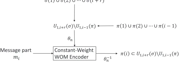
same way, for eachiin [1 :q₋r₋1], the set of candidate cells forπ(i) isU1,i+r(σ)\U1,i−1(π).

Message part

݉௜

Constant-Weight

WOM Encoder ߨ ݅ ؿ ܷଵǡ௜ା௥ሺߪሻ̳ܷଵǡ௜ିଵሺߨሻ ߨ ͳ ׫ ߨሺʹሻ ׫ ڮ ׫ ߨ ݅ െ ͳ ߪ ͳ ׫ ߪ ʹ ׫ ڮ ׫ ߪሺ݅ ൅ ݎሻ

ܷଵǡ௜ା௥ሺߪሻ̳ܷଵǡ௜ିଵሺߨሻ

ߠ௡

ߠ௡ିଵ

Figure 3.1: Iteration i of the encoding algorithm, where 1_≤i_≤q₋r₋1.

Construction 3.2: (A RM rewriting code from a constant-weight strong WOM code) Let KW, q, r, z be positive integers, let n = qz and let (EW, DW) be an (n, KW,(r+ 1)/q,1/q) constant-weight strong WOM coding scheme. Define the multiset

M = {(q−r)z_{,(q−r+ 1)}z_{, . . . , q}z_{} and let K}

M = |SM| and KR = KWq−r−1 ·KM. The

codebook _C is defined to be the entire set S_{q,z. A (q, z, KR, r) RM rewrite coding scheme}

{ER, DR} is constructed as follows:

The encoding algorithm ER receives a message m= (m1, m2, . . . , mq−r)∈[KW]q−r−1× [KM] and a state permutation σ∈Sq,z, and returns a permutation π in Bq,z,r(σ)∩D−R1(m)

to store in the memory. It is constructed as follows:

1: for i= 1 to q−r−1 do 2: si ⇐θn(U1,i+r(σ)\U1,i−1(π))

3: xi ⇐EW(mi,si)

4: π(i)⇐θ_n−1(xi)

5: end for

6: π_[q−r:q]⇐h_M(m_q−r)

The decoding algorithm DR receives the stored permutation π ∈ Sq,z, and returns the

stored message m= (m1, m2, . . . , mq−r)∈[KW]q−r−1×[KM]. It is constructed as follows:

1: for i= 1 to q−r−1 do 2: xi ⇐θn(π(i))

4: end for

5: mq−r ⇐h−M1(π[q−r:q])

Theorem 3.1: Let _{EW, DW} be a member of an efficient capacity-achieving family of

constant-weight strong WOM coding schemes. Then the family of RM rewrite coding schemes

in Construction 3.2 is efficient and capacity-achieving.

Proof: The decoded message is equal to the encoded message by the property of the WOM code in Definition 3.1. By the explanation above the construction, it is clear that the cost is bounded byr, and therefore_{ER, DR}is a RM rewrite coding scheme. We will first show that

{ER, DR} is capacity achieving, and then show that it is efficient. Let RR = (1/n) logKR be the rate of a RM rewriting code. To show that _{ER, DR} is capacity achieving, we need to show that for any ǫR>0, RR> CR−ǫR, for some q and z.

Since _{EW, DW}is capacity achieving, RW > CW −ǫW for anyǫW >0 and large enough

n. Remember that CW =wsH(wx/ws). In {ER, DR} we use ws = (r+ 1)/q and wx = 1/q, and so CW = r+1_q H _r+11

. We have

RR = (1/n) logKR

= (1/n) log(KM ·KWq−r−1)

>(q₋r₋1)(1/n) logKW

>(q₋r₋1)(CW −ǫW) (3.1)

= (q₋r₋1)

r+ 1

q H

1

r+ 1

−ǫW

= q−r−1

q (CR−qǫW)

= (CR−qǫW)(1−(r+ 1)/q)

The idea is to take q=⌊(r+ 1)/√ǫW⌋ and ǫR= 3(r+ 1)√ǫW, and get that

RR > CR−

(r+ 1)2

⌊(r+ 1)/√ǫW⌋−⌊

(r+ 1)/√ǫW⌋ǫW > CR−2(r+ 1)√ǫW−(r+ 1)√ǫW =CR−ǫR.

Formally, we say: for anyǫR>0 and integerr, we set ǫW = ǫ

2

R

9(r+1)2 and q=⌊(r+ 1)/√ǫW⌋. Now if z is large enough then n =qz is also large enough so that RW > CW −ǫW, and then Equation 3.1 holds and we have RR > CR−ǫR, proving that the construction is capacity achieving. Note that the family of coding schemes has a constant value of q and a growing value of z, as permitted by Definition 2.2 of capacity-achieving code families.

Next we show that _{ER, DR} is efficient. If the scheme (hM, h−M1) is implemented as described in [60], then the time complexity of hM and h−M1 is polynomial in n. In addition, we assumed thatEW andDW run in polynimial time inn. So sincehM andh−M1 are executed only once in ER and DR, and EW and DW are executed less than q times in ER and DR, where q < n, we get that the time complexity of ER and DR is polynomial in n.

3.1.5

How to Use Weak WOM Schemes

As mentioned earlier, we are not familiar with a family of efficient capacity-achieving constant-weight strong WOM coding schemes. Nonetheless, it turns out that we can construct effi-cient capacity-achieving WOM coding schemes that meet a slightly weaker definition, and use them to construct capacity-achieving RM rewriting codes. In this subsection we will define a weak notion of constant-weight WOM codes, and describe an associated RM rewrit-ing codrewrit-ing scheme. In Sections 3.2 and 3.3 we will present yet weaker definition of WOM codes, together with constructions of appropriate WOM schemes and associated RM rewrit-ing schemes.

codeword. This allows the encoder to communicate some information to the decoder without restrictions.

Definition 3.2: (Constant-weight weak WOM codes) LetKW, Ka, n be positive

inte-gers and let ws be a real number in [0,1] and wx be a real number in [0, ws]. A surjective

function DW : Jwx(n)×[Ka] → [KW] is an (n, KW, Ka, ws, wx) constant-weight weak

WOM code if for each message m _∈[KW] and state vector s∈Jws(n), there exists a pair

(x, ma)in the subsetD−_W1(m)⊆Jwx(n)×[Ka]such thatx≤s. The rate of a constant-weight

weak WOM code is defined as RW = (1/n) log(KW/Ka).

If Ka = 1, the code is in fact a constant-weight strong WOM code. We will only be interested in the case in which KW ≫ Ka. Since RW is a decreasing function of Ka, it follows that the capacity of constant-weight weak WOM code is also CW = wsH(wx/ws). Consider now the encoderERof a (q, z, KR, r) RM rewriting codeDRwith a codebookC. For a messagem_∈[KR] and a state permutationσ_{∈ C}, the encoder needs to find a permutation

π in the intersection Bq,z,r(σ)∩D−_R1(m). As before, we let the encoder determine the sets

π(1), π(2), . . . , π(q₋r₋1) sequentially, such that each setπ(i) represents a message partmi. If we were to use the previous encoding algorithm (in Construction 3.2) with a weak WOM code, the WOM encoding would find a pair (xi, ma,i), and we could store the vector xi by the set π(i). However, we would not have a way to store the index ma,i that is also required for the decoding. To solve this, we will add some cells that will serve the sole purpose of storing the index ma,i.

r. We also let the number of cells in each rank in those added sets to be equal, in order to maximize the amount of stored information. Denote the number of cells in each rank in each of the added sets as a. Since each added set needs to store an index from the set [Ka] with

r+ 1 ranks, it follows that a must satisfy the inequality _|S_{r+1,a| ≥Ka. So to be economical}

with our resources, we setato be the smallest integer that satisfies this inequality. We denote each of these additional permutations asπa,i ∈Sr+1,a. The main permutation is denoted by

πW, and the number of cells in each rank inπW is denoted byzW. The permutationπwill be a string concatenation of the main permutation together with theq₋r₋1 added permutations. Note that this way the number of cells in each rank is not equal (there are more cells in the lowest r+ 1 ranks). This is actually not a problem, but it will be cleaner to present the construction if we add yet another permutation that “balances” the code. Specifically, we letπb be a permutation of the multiset

(r+ 2)(q−r−1)a_{,(r+ 3)}(q−r−1)a_{, . . . , q}(q−r−1)a _{and let}

π−1 _{be the string concatenation (π}−1

a,1, . . . , πa,q−1−r−1, π−b1, πW−1). This way in each rank there are exactly zW + (q−r−1)a cells. We denotez =zW + (q−r−1)a, and then we get that

π is a member of S_q,z.

On each iteration i from 1 to q ₋r ₋ 1 we use a constant-weight weak WOM code. The vectors si and xi of the WOM code are now corresponding only to the main part of the permutation, and we denote their length bynW =qzW. We assign the state vector to besi =

θnW(U1,i+r(σW)\U1,i−1(πW)), where σW andπW are the main parts ofσ and π, accordingly.

Note that U1,i+r(σW) and U1,i−1(πW) are subsets of [nW] and that the characteristic vector

θnW is taken according to nW as well. The message part mi and the state vector si are

used by the encoder EW of an (nW, KW, Kb,(r + 1)/q,1/q) constant-weight weak WOM code DW. The result of the encoding is the pair (xi, ma,i) = EW(mi,si). The vector

xi is stored on the main part of π by assigning πW(i) = θ−nW1(xi). The additional index

ma,i is stored on the additional cells corresponding to rank i. Using an enumerative code

hr+1,a : [|Sr+1,a|]→Sr+1,a, we assign πa,i=hr+1,a(ma,i). After the lowestq−r−1 ranks of

πW are determined, we determine the highest r+ 1 ranks by setting πW,[q−r,q] =hM(mq−r) where M = _{(q₋r)zW_{,(q−r+ 1)}zW_{, . . . , q}zW_{}. Finally, the permutation π}