http://dx.doi.org/10.4236/ajcm.2014.43014
Supersonic Flutter of a Spherical Shell
Partially Filled with Fluid
Mohamed Menaa, Aouni A. Lakis
Department of Mechanical Engineering, Ecole Poly Technique de Montreal, Montréal, Canada Email: [email protected]
Received 28 November 2013; revised 28 January 2014; accepted 5 February 2014 Copyright © 2014 by authors and Scientific Research Publishing Inc.
This work is licensed under the Creative Commons Attribution International License (CC BY). http://creativecommons.org/licenses/by/4.0/
Abstract
In the present study, a hybrid finite element method is applied to investigate the dynamic beha-
vior of a spherical shell partially filled with fluid and subjected to external supersonic airflow. The
structural formulation is a combination of linear spherical shell theory and the classic finite
ele-ment method. In this hybrid method, the nodal displaceele-ments are derived from exact solution of spherical shell theory rather than approximated by polynomial functions. Therefore, the number of elements is a function of the complexity of the structure and it is not necessary to take a large number of elements to get rapid convergence. Linearized first-order potential (piston) theory with
the curvature correction term is coupled with the structural model to account for aerodynamic loading. It is assumed that the fluid is incompressible and has no free surface effect. Fluid is
con-sidered as a velocity potential at each node of the shell element where its motion is expressed in terms of nodal elastic displacements at the fluid-structure interface. Numerical simulation is done
and vibration frequencies are obtained. The results are validated using numerical and theoretical data available in literature. The investigation is carried out for spherical shells with different boundary conditions, geometries, filling ratios, flow parameters, and radius to thickness ratios. Results show that the spherical shell loses its stability through coupled-mode flutter. This pr
o-posed hybrid finite element method can be used efficiently for analyzing the flutter of spherical shells employed in aerospace structures at less computational cost than other commercial FEM software.
Keywords
Vibration, Spherical shell, Flutter, Hybrid FEM
1. Introduction
Their applications include the propellant tank or gas-deployed skirt of spacecraft. Due to the aerodynamic shape combined with thin wall thicknesses, spherical shells are more disposed to dynamic instability or flutter induced by high Mach number gas flow. It is therefore important to understand the effect of different flow parameters and loadings on their aeroelastic response.
Aeroelastic analysis of shells and plates has been studied by numerous researchers experimentally and analyt-ically [1]. Dowell gives an exhaustive study of the aeroelasticity of shells and plates in his book [2]. After in-troducing the application of piston theory in the aeroelastic modeling presented by Ashley and Zatarian [3], a number of interesting experimental and theoretical studies were carried out to investigate supersonic flutter of cylindrical shells. In general, all of this research was concerned with the development of an analytical relation to describe the effect of shell and flow parameters on the critical flutter dynamic pressure. Aeroelastic models in combination with linear or nonlinear piston theory were coupled to the theory of shells to account for fluid- structure interaction. The resulting governing equations were treated numerically using the Galerkin method. A comprehensive experimental test was done by Fung and Olson [4]. They studied the effects of shell boundary conditions and initial stress state due to internal pressure and axial load. It was observed that pressurized cylin-drical shell fluttered at a lower level of freestream static pressure than predicted by theory [5]. Later, Evensen and Olson [6] [7] presented a nonlinear analysis to take account of this observed effect. Dowell [8] also analyzed the behavior of a cylindrical shell in supersonic flow for different flow and shell parameters. A complete de-scription of panel flutter modeling is given in his book [2]. A study by Carter and Strearman [9] showed that agreement between the theory and experiments reported in the literature exists in cases that involve a small amount of static preload acting on the shell. Amabili and Pellicano [10] included geometric nonlinearities in their study of supersonic flutter of a circular cylindrical shell. By selecting expansion modes to discretize the aeroelastic equations, they were able to facilitate their solution, and therefore succeeded in capturing the nonli-near behavior of the shell correctly.
There are also some researchers who focused their efforts on the numerical study of this problem. The equa-tions of virtual displacements were solved using the finite elements method. Aeroelastic governing equaequa-tions were formulated by applying classical shell theory coupled with the piston theory for evaluation of aerodynamic forces. For example, Bismarck-Nasr [11] developed a FEM applied to supersonic flutter of circular shell sub-jected to internal pressure and axial loading. Ganapathi et al. [12] modeled an orthotropic and laminated aniso-tropic cylindrical shell in supersonic flow using FEM and analyzed the effect of different shell geometries on the flutter boundaries.
Aeroelasticity of conical shells has also been investigated by few researchers. The leading work in this field was conducted by Shulman [13]. Ueda et al. [14] investigated theoretically and experimentally the supersonic flutter of a conical shell. Dixon and Hudson [15] studied the flutter and vibration of an orthotropic conical shell theoretically. Miserentino and Dixon [16] investigated experimentally the vibration and flutter of a pressurized truncated conical shell. Bismarck-Nasr and Costa-Savio [18] studied the supersonic flutter of conical shells us-ing finite element method. Sunder et al. [18] successfully applied the finite element analysis to calculate the flutter of a laminated conical shell. In another study they found the optimum cone angle in aeroelastic flutter [19]. Mason and Blotter [20] used a finite element technique to find the flutter boundary for a conical shell (a typical rocket nozzle element) subjected to an internal supersonic gas flow. Pidaparti and Yang Henry [21] completed a theoretical study to predict the onset of flutter instability for composites conical shells.
2. Formulation
2.1. Structural Modeling
2.1.1. Equilibrium Equations
In this study the structure is modeled using hybrid finite element method which is a combination of spherical shell theory and classical finite element method. In this hybrid finite element method, the displacement functions are found from exact solution of spherical shell theory rather than approximated by polynomial functions as done in classical finite element method. In the spherical coordinate system (R, θ, ϕ) shown inFigure 1, five out of the six equations of equilibrium derived in reference [22] for spherical shells are written as follows:
(
)
(
)
(
)
1
cot 0
sin 1
2 cot 0
sin 1
cot 0
sin 1
cot 0
sin 1
2 cot 0
sin
N N
N N Q
N N
N Q
Q Q
Q N N
M M
M M RQ
M M
M RQ
φ φθ
φ θ φ
φθ θ
φθ θ
φ θ
φ φ θ
φ φθ
φ θ φ
φθ θ
φθ θ
φ
φ φ θ
φ
φ φ θ
φ
φ φ θ
φ
φ φ θ
φ
φ φ θ
∂ ∂
+ + − + =
∂ ∂
∂ ∂
+ + + =
∂ ∂
∂ ∂
+ + − + =
∂ ∂
∂ ∂
+ + − − =
∂ ∂
∂ ∂
+ + − =
∂ ∂
(1)
where Nφ, Nθ, Nφθ are membrane stress resultants; Mϕ, Mθ, Mϕθthe bending stress resultants and Qϕ, Qθthe shear forces (Figure 2). The sixth equation, which is an identity equation for spherical shells, is not presented here.
2.1.2. Constitutive Relations
Strains and displacements in axial, Uφ, radial, W, and circumferential, Uθ directions are related as follows:
Figure 2. Stress resultants and stress couple.
{ }
22 2
2
2 2 2
2
1
1 1
cot sin
1 1
cot sin
2
1 2
1 1 1
cot cot
sin sin
1 1
sin
U W R
U
U W
R
U U
U R
U W
R
U W W
U R
U U
R
φ
θ φ φ
φ θ
θ
θ φθ
φ φ
θ
φθ
θ φ
φ θ
φ
φ φ θ
ε
ε φ
φ φ θ
ε
ε κ
κ φ φ
κ
φ φ
φ θ φ θ φ
φ φ
∂
+
∂
∂
+ +
∂
∂ ∂
+ −
∂ ∂
= =
∂
∂
−
∂ ∂
∂ + − ∂ − ∂
∂ ∂ ∂
∂ ∂
+ ∂
2
1 1
cot 2 cot 2
sin sin
W W
Uθ φ φ
θ φ θ φ φ θ
∂ ∂
− + −
∂ ∂ ∂ ∂
(2)
Displacements U , W and V in the global Cartesian coordinate system are related to displacements Uφi,
i
W And Uθi indicated inFigure 3 by:
sin cos 0 cos sin 0
0 0 1
i i i
i i i
i
U U
W W
V U
φ
θ
φ φ
φ φ
−
=
(3)
The stress vector
{ }
σ is expressed as a function of strain{ }
ε by:Figure 3. Spheical frustum element.
[ ]
11 12 14 15
21 22 24 25
33
41 42 44 45
51 52 54 55
36 66
0 0
0 0
0 0 0 0 0
0 0
0 0
0 0 0 0
P P P P
P P P P
P P
P P P P
P P P P
P P
=
(5)
Upon substitution of Equations (2), (4) and (5) into Equation (1), a system of equilibrium equations can beobtained as a function of displacements:
(
)
(
)
(
)
1
2
3
, , , 0 , , , 0 , , , 0
ij ij ij
L U W U P
L U W U P
L U W U P
φ θ
φ θ
φ θ
= = =
(6)
These three linear partial differential operators L1, L2 and L3 are given in Appendix A, and Pij are ele-ments of the elasticity matrix, which for an isotropic thin shell with thickness h is given by:
[ ]
(
)
(
)
0 0 0 0
0 0 0 0
1
0 0 0 0 0
2
0 0 0 0
0 0 0 0
1
0 0 0 0 0
2
D D
D D
D
P
K K
K K
K
ν ν
ν
ν ν
ν
−
=
−
where 2 1
Eh D
ν =
− is the membrane stiffness and
(
)
3
2 12 1
Eh K
ν
=
− is the bending stiffness.
2.1.3. Kinematic Relations
The element is a circumferential spherical frustum shown inFigure 3. It has two nodal circles with four degrees of freedom; axial, radial, circumferential and rotation at each node. This element type makes it possible to use thin shell equations easily to find the exact solution of displacement functions rather than an approximation with polynomial functions as done in classical finite element method.
For motions associated with the circumferential wave number n, we may write:
( )
( )
( )
( )
( )
( )
[ ]
( )
( )
( )
, cos 0 0
, 0 cos 0
, 0 0 sin
n n
n n
n n
U n u u
W n w T w
U n u u
φ φ φ
θ θ θ
φ θ θ φ φ
φ θ θ φ φ
φ θ θ φ φ
= =
(8)
The transversal displacement wn
( )
φ can be expressed as [22]:( )
3 1n
n i
i
w φ w
=
=
∑
(9)where
(
cos)
(
cos)
i i
n n n
i i i
w =A Pµ
φ
+B Qµφ
(10) and where Pµni(
cosφ)
, i(
cos)
n
Qµ
φ
are the associated Legendre functions of the first and second kindsrespec-tively of order n and degree µi.
The expression of the axial displacement uϕν(ϕ) is:
( )
3 2( )
1 d
d 2 sin
n i
n i
i
w n
uφ φ E ψ φ
φ φ
=
=
∑
− (11)where the coefficient Ei is given by:
(
) (
)
(
)(
)
1 1
1 1
i i
i
k E
k
λ ν ν
λ ν
+ + − −
=
+ − + (12)
The auxiliary function ψ is given by the expression:
( )
4 1(
cos)
4 1(
cos)
n n
A P B Q
ψ φ = φ + φ (13)
Finally the circumferential displacement uϕν(ϕ) can be expressed as:
( )
3 11 d
sin 2 d
n
n i i
i
n
uθ φ n E w ψ
φ φ
=
= −
∑
+ (14)The degree µi is obtained from the expression
1 2
1 1
4 2
i i
µ = +λ −
(15) where λi is one the roots of the cubic equation:
3 2
1 2 3 0
h h h
λ − λ + λ− = (16) and where
(
)
(
)
(
)
(
)
1
2 2
2 3
4
4 1 1
2 1 1 h
h k
h k
ν ν
=
= + + −
= + −
with
2
2 12R
k h
= .
The above equation has three roots with one real root and two others complex conjugates. The Legendre functions Pµn1, 1 1 1
1 1
, and
n n n
Pµ− Qµ Qµ− are real functions whereas Pµni, Pµni−1,Qµni and Qµni−1
(i = 2, 3) are complex functions. So we can put:
( )
( )
( )
( )
( )
( )
( )
( )
( )
( )
( )
( )
( )
( )
( )
( )
2 2 2
3 2 2
2 2 2
3 2 2
2 2 2
3 2 2
2 2 2
3 2 2
1 1 1
1 1 1
1 1 1
1 1 1
Re i Im
Re i Im
Re i Im
Re i Im
Re i Im
Re i Im
Re i Im
Re i Im
n n n
n n n
n n n
n n n
n n n
n n n
n n n
n n n
P P P
P P P
Q Q Q
Q Q Q
P P P
P P P
Q Q Q
Q P Q
µ µ µ
µ µ µ
µ µ µ
µ µ µ
µ µ µ
µ µ µ
µ µ µ
µ µ µ
− − −
− − −
− − −
− − −
= +
= −
= +
= −
= +
= −
= +
= −
(18)
Setting
(
)(
)
(
)(
)
(
)(
)
1 1 1
2 2 2 3
3 3 2 3
1
1 i
1 i
n n c
n n c c
n n c c
µ µ
µ µ
µ µ
− − + =
− − + = +
− − + = −
(19)
1 1
2 2 3
3 2 3
i i
E e
E e e
E e e
=
= −
= +
(20)
Substituting Equations (18), (19) and (20) in Equations (9), (11) and (14) we have:
( )
(
)
( )
( )
(
)
( )
(
)
( )
(
)
( )
( )
(
)
( )
(
)
( )
(
)
1 1
2 2 2 2
2 2 2 2
1
1 1 1 1
1 1
2 3 2 2 3 3 3 2 2 3 2 3
1 1
3 2 3 2 2 3 2 2 3 3 2 3
2
1 4
cot
cot Re cot Im Re Im
cot Re cot Im Re Im i
2 sin
n n
n
n n n n
n n n n
n
u ne P e c P A
ne P ne P e c e c P e c e c P A A
ne P ne P e c e c P e c e c P A A
n
P A
φ µ µ
µ µ µ µ
µ µ µ µ
φ φ
φ φ
φ φ
φ
−
− −
− −
= − +
+ − − + + + − +
+ − − − + + −
+ − + −
(
)
( )
( )
(
)
( )
(
)
( )
(
)
( )
( )
(
)
( )
(
)
( )
(
)
1 1
2 2 2 2
2 2 2 2
1
1 1 1 1
1 1
2 3 2 2 3 3 3 2 2 3 2 3
1 1
3 2 3 2 2 3 2 2 3 3 2 3
2
1 4
cot
cot Re cot Im Re Im
cot Re cot Im Re Im i
2 sin
n n
n n n n
n n n n
n
ne Q e c Q B
ne Q ne Q e c e c Q e c e c Q B B
ne Q ne Q e c e c Q e c e c Q B B
n
Q B
µ µ
µ µ µ µ
µ µ µ µ
φ
φ φ
φ φ
φ
−
− −
− −
+
+ − − + + + − +
+ − − − + + −
+ −
( )
( )
(
)
( )
(
)
( )
(
)
( )
(
)
1 2
2 1
2 2
1 2 3
2 3 1
2 3 2 3
Re Im i
Re Im i
n n
n
n n
n n
w P A P A A
P A A Q B
Q B B Q B B
µ µ
µ µ
µ µ
φ = + +
+ − +
+ + + −
( )
( )
( )
(
)
( )
( )
(
)
(
)(
)
( )
( )
(
)
1 2 2 2
2 2 2
1
2 2 2
1 1 3 2 3
3 2 3
2
1
1 1 4 1 1
3 2 3
3
1 1 1
Re Im
sin sin sin
1 1
Re Im i
sin sin
1
cot 2 1
2 2 sin
1 1
Re Im
sin sin
1 si
n n n
n
n n
n n n
n n
u ne P A ne P ne P A A
ne P ne P A A
n n
P n n P A ne Q B
ne Q ne Q B B
ne
θ µ µ µ
µ µ
µ
µ µ
φ
φ φ φ
φ φ φ φ φ φ − = − − + + + − − + − + − + − − + + +
( )
( )
(
)
(
)(
)
2 2 2 2 3
2
1
1 1 4
1
Re Im i
n sin
cot 2 1
2 2
n n
n n
Q ne Q B B
n n
Q n n Q B
µ µ φ φ φ − − − + − + − +
In deriving the above relation we used the recursive relations:
(
)(
)
(
)(
)
1 1 d cot 1 d d cot 1 d i i i i i i n n n i i n n n i i Pn P n n P
Q
n Q n n Q
µ
µ µ
µ
µ µ
φ µ µ
φ
φ µ µ
φ − − = − + − − + = − + − − + (22)
Using matrix formulation, the displacement functions can be expressed as follows:
( )
( )
( )
[ ]
( )
( )
( )
[ ][ ]
{ }
, , , n n n U uW T w T R C
U u
φ φ
θ θ
φ θ φ
φ θ φ
φ θ φ
= = (23)
The vector
{ }
C is given by the expression:{ }
T{
(
)
(
)
}
1 2 3 i 2 3 4 1 2 3 i 2 3 4
C = A A +A A −A A B B +B B −B B (24)
The elements of matrix
[ ]
R are given in Appendix B.In the finite element method, the vector C is eliminated in favor of displacements at elements nodes. At each finite element node, the three displacements (axial, transversal and circumferential) and the rotation are applied. The displacement of node i are defined by the vector:
{ }
T d
d
i i i n i
i n n n
w
uφ w uθ
δ φ =
(25)
The finite element shown in Figure 3 with two nodal lines (i and j) and eight degrees of freedom will have the following nodal displacement vector:
[ ]{ }
T
d d
d d
i j
i i i n i j j n j
n n n n n n
j
w w
uφ w uθ uφ w uθ A C
δ
δ φ φ
= =
(26)
with
(
)
( )
( )
( )
(
)
( )
( )
( )
(
)
(
)
( )
( )
( )
(
)
( )
1 1 2 2 2
2 2 2 1 1
2 2 2
2
1 1 1
1 1 2 3 2 3
1 1 1
3 2 2 3 1 1
1 1
2 3 2 3
3 d
cot cot Re Re Im
d
cot Im Re Im i cot
cot Re Re Im
cot Im Re
n n n n n
n
n n n n n
n n n
n
w
n P c P A n P c P c P A A
n P c P c P A A n Q c Q B
n Q c Q c Q B B
n Q c
µ µ µ µ µ
µ µ µ µ µ
µ µ µ
µ φ φ φ φ φ φ φ − − − − − − − − = − + + − + − + + − + + − + − + + − + − + + − +
( )
( )
(
)
2 2 1 12Im i 2 3
n n
Qµ− c Qµ− B B
+ −
The terms of matrix, obtained from the values of matrix
[ ]
R and d dn
w
x , are given in Appendix B. Now,
pre-multiplying Equation (26) by
[ ]
A−1 one obtains the matrix of the constant Ci as a function of the degree offreedom:
{ }
[ ]
1 ij
C = A − δδ
(28) Finally, one substitutes the vector
{ }
C into Equation (26) and obtains the displacement functions as fol-lows:( )
( )
( )
[ ][ ][ ]
[ ]
1 ,
, ,
i i
j j
U
W T R A N
U
φ
θ
φ θ δ δ
φ θ δ δ
φ θ
−
= =
(29)
The strain vector
{ }
ε can be determined from the displacement functions U U Wφ, θ, and the deformation –displacement equation (2) as:{ }
[ ] [ ]
[ ] [ ] [ ]
0{ }
[ ] [ ]
[ ] [ ] [ ][ ]
0 1[ ]
0 0
i i
j j
T T
Q C Q A B
T T
δ δ
ε − δ δ
= = =
(30)
where matrix
[ ]
Q is given in Appendix C.2.1.4. Mass and Stiffness Matrices
This relation can be used to find the stress vector, Equation (4), in terms of the nodal degrees of freedom vector:
{ }
[ ][ ]
i jP B δ
σ = δ
(31) Based on the finite element formulation, the local stiffness and mass matrices are:
[ ]
[ ] [ ][ ]
[ ]
[ ] [ ]
T
T d
d
loc A
loc A
k B P B A
m ρh N N A
=
=
∫∫
∫∫
(32)where ρ is the density and h is the thickness of shell.
The surface element of the shell wall is dA=R2sin d dφ φ θ (Figure 2). After integrating over θ, the pre-ceding equations become
[ ]
[ ] [ ][ ]
[ ]
T T
1 2 1
T
1 1
π sin d
j
i
loc
k A R Q P Q A
A G A
φ
φ
φ φ
− −
− −
=
=
∫
[ ]
[ ] [ ]
[ ]
T T
1 2 1
T
1 1
π sin d
j
i
loc
m h A R R R A
h A S A
φ
φ
ρ φ φ
ρ
− −
− −
=
=
∫
(33)
In the global system, the element stiffness and mass matrices are
[ ] [ ]
[ ]
[ ]
[ ]
[ ]
[ ]
[ ]
T
T 1 1
T
T 1 1
k LG A G A LG
m ρh LG A S A LG
− −
− −
=
where
[ ]
sin cos 0 0 0 0 0 0
cos sin 0 0 0 0 0 0
0 0 1 0 0 0 0 0
0 0 0 1 0 0 0 0
0 0 0 0 sin cos 0 0
0 0 0 0 cos sin 0 0
0 0 0 0 0 0 1 0
0 0 0 0 0 0 0 1
i i
i i
j j
j j
LG
φ φ
φ φ
φ φ
φ φ
−
= −
(35)
From these equations, one can assemble the mass and stiffness matrices for each element to obtain the mass and stiffness matrices for the whole shell:
[ ]
M and[ ]
K . Each elementary matrix is 8 × 8, therefore the final dimensions of[ ]
M and[ ]
K will be 4*(N + 1) where N is the number of elements of the shell.2.2. Aerodynamic Modeling
Piston theory, introduced by Ashley and Zartarian [3], is a powerful tool for aeroelasticity modeling. In this study the fluid-structure effect due to external pressure loading can be taken into account using linearized first- order potential theory. This pressure is expressed as:
(
)
(
)
2 2
1 2 2 1 2
2 2
2 1 1
1 2 1
a
m
P M W M W W
P
R M U t
M R M
γ
φ
∞
∞
∂ − ∂
= − + −
∂ − ∂
− − (36)
where P∞,U∞, M and γ are the freestream static pressure, freestream velocity, Mach number and adiabatic exponent of air respectively. If the Mach number is sufficiently high
(
M≥2)
, and curvature term,(
2)
1 22 m 1
W R M − is neglected, the result is the so-called piston theory:
1
a
M W W
P P
R a t
γ
φ
∞
∞
∂ ∂
= − +
∂ ∂
(37)
where a∞ is the free stream speed of sound.
Finally, the aerodynamic pressure in terms of radial displacement is written:
(
)
(
)
2 3 2
1 2 2 1 2
2 1 2
d
1 2 1 1
d 1
1 2 1
j
a j j
j
m
W
U M
P W W
U M R
M M R
ρ
φ
∞ ∞
= ∞
−
= − + −
−
−
∑
− (38)and the pressure loading in terms of nodal degrees of freedom is written as:
{ }
(
)
[ ]
(
)
[ ]
(
) (
)
[ ]
2 2
1 1
1 2 2
2
2
1 2 1 2
2
2
1 1
1 2 1 2
2 2
0
1 2
1 1
0
1 1
1
1 2 1
i a
a r
j
i a
j
i a
j m
U M
P P T R A
U M
M
U
T R A
R M
U
T R A
M M R
δ ρ
δ
δ ρ
δ
δ ρ
δ
−
∞ ∞
∞
−
∞ ∞
−
∞ ∞
−
= = −
−
−
−
−
+
− −
where ρ∞ the freestream air density and Rm is the median radius for each element. Based on thermodynamic
U∞ =Ma∞ (39)
P
a γ
ρ∞
∞
∞
= (40)
The matrix 1
a
R
is given by:
( )
( )
( )
( )
1 2 2 1 2 2
1
0 0 0 0 0 0 0 0
Re Im 0 Re Im 0
0 0 0 0 0 0 0 0
a n n n n n n
R Pµ Pµ Pµ Qµ Qµ Qµ
=
(41)
The matrix 2
a
R
is given by:
( )
( )
( )
( )
( )
( )
( )
( )
[ ]
1 2 2 1 2 2
1 2 2 1 2 2
2
1 1 1 1 1 1
0 0 0 0 0 0 0 0
cot Re Im 0 Re Im 0
0 0 0 0 0 0 0 0
0 0 0 0 0 0 0 0
Re Im 0 Re Im 0
0 0 0 0 0 0 0 0
a n n n n n n
n n n n n n
R n P P P Q Q Q
P P P Q Q Q C
µ µ µ µ µ µ
µ µ µ µ µ µ
φ
− − − − − −
= −
+
(42)
where matrix
[ ]
C is given by:[ ]
1
2 3
3 2
1
2 3
3 2
0 0 0 0 0 0 0
0 0 0 0 0 0
0 0 0 0 0 0
0 0 0 0 0 0 0 0
0 0 0 0 0 0 0
0 0 0 0 0 0
0 0 0 0 0 0
0 0 0 0 0 0 0 0
c
c c
c c
C
c
c c
c c
−
=
−
(43)
The general force vector due to a pressure field is written as:
{ }
[ ]
T{ }
d
p a
A
F =
∫∫
N P A (44) The local damping matrix is given by:(
)
[ ]
(
)
2 2
T T
1 2 1
1
1 2 2
2
2 2
T
1 1
1 2 2
2
1 2
π sin d
1 1
1 2
1 1
j
i
a f loc
f
U M
c A R R R A
U M
M
U M
A D A
U M
M
φ
φ
ρ φ φ
ρ
− −
∞ ∞
∞
− −
∞ ∞
∞
−
= −
−
−
−
= −
− −
∫
(45)
Finally the local stiffness matrix is given by:
(
)
[ ]
(
)
[ ]
(
)
2
T T T
1 2 2 1
2 1
1 2 1 2
2 2
2
T
1 1
1 2 2
1
π sin d π sin d
1 2 1
1
j j
i i
a a
f loc
m
f
U
k A R R R R R R A
M M R
U
A G A
M
φ φ
φ φ
ρ φ φ φ φ
ρ
− −
∞ ∞
− −
∞ ∞
= − −
− −
= −
−
In the global system, the element damping and stiffness matrices are:
(
)
[ ]
[ ]
(
)
[ ]
[ ]
2 2
T
T 1 1
1 2 2
2
2
T
T 1 1
1 2 2
1 2
1 1
1
f f
f f
U M
c LG A D A LG
U M
M
U
k LG A G A LG
M
ρ
ρ
− −
∞ ∞
∞
− −
∞ ∞
−
= −
−
−
= −
−
(46)
From these equations, one can assemble the damping and stiffness matrices for each element to obtain the damping and stiffness matrices for the whole shell: Cf and Kf.
2.3. Fluid Modeling
The Laplace equation satisfied by velocity potential for inviscid, incompressible and irrotational fluid in the spherical system is written as:
2
2 2
2 2 2 2 2
1 1 1
sin 0
sin sin
r
r r
r r r
ϕ ϕ ϕ
ϕ φ
φ φ
φ φ θ
∂ ∂ ∂ ∂ ∂
∇ = + + =
∂ ∂ ∂ ∂ ∂ (47)
where the velocity components are:
1 1
, ,
sin
r
V V V
r r r
φ ϕφ ϕ θ φ θϕ
∂ ∂ ∂
= = =
∂ ∂ ∂ (48)
Using the Bernouilli equation, hydrodynamic pressure in terms of velocity potential
ϕ
and fluid densityρ
fis found as:
f f
r R
P
t
ϕ ρ
= ∂
= −
∂
(49)
The impermeability condition, which ensures contact between the shell surface and the peripheral fluid, is written as:
r r R
r R r R
W V
r t
ϕ
=
= =
∂ ∂
= =
∂ ∂ (50)
with
(
)
(
)
(
)
3
i 1
cos cos cos e
j j
n n t
j j
j
W A Pµ φ B Qµ φ nθ ω
=
=
∑
+ (51)Method of separation of variables for the velocity potential solution can be done as follows:
(
)
3( ) (
)
1
, , j j , ,
j
r R r S t
ϕ φ θ φ θ
=
=
∑
(52)Placing this relation into the impermeability condition (50), we can find the function Sj
(
φ θ, ,t)
in term of radial displacement:(
)
1( )
, , j
j
j r R
W
S t
R R t
φ θ
= ∂ =
′ ∂ (53)
Hence the equation becomes
(
)
3( )
( )
1
, , j j
j j r R
R r W
r
R R t
ϕ φ θ
= =
∂ =
′ ∂
∑
(54)( )
( )
(
2)
( )
1 20
j j
j j j
R r R r R r
r r
µ µ +
′′ + ′ − = (55)
Solution of the above differential equation yields the following:
( )
jj
j j j
B
R r A r
r µ
µ
= + (56)
For internal flow Bj =0
Finally, the hydrodynamic pressure in terms of radial displacement is written:
3
1
f f j
j j
R
P ρ W
µ
=
= −
∑
(57)We put:
1 1
2 3
2
2 3
3 i
i R
f
R
f f
R
f f
µ
µ
µ
=
= −
= +
(58)
And the pressure loading in terms of nodal degrees of freedom is written as:
{ }
[ ]
11 0
0
i f
f f
j
P P ρ T R A δ
δ
−
= = −
(59)
where matrix 1
f
R
is given by:
( )
( )
( )
( )
[ ]
1 2 2 1 2 2
1
0 0 0 0 0 0 0 0
Re Im 0 Re Im 0
0 0 0 0 0 0 0 0
f n n n n n n
R Pµ Pµ Pµ Qµ Qµ Qµ F
=
(60)
where
[ ]
F is expressed as:[ ]
1
2 3
3 2
1
2 3
3 2
0 0 0 0 0 0 0
0 0 0 0 0 0
0 0 0 0 0 0
0 0 0 0 0 0 0 0
0 0 0 0 0 0 0
0 0 0 0 0 0
0 0 0 0 0 0
0 0 0 0 0 0 0 0
f
f f
f f
F
f
f f
f f
−
=
−
(61)
The general force vector due the fluid pressure loading is given by:
{ }
[ ]
T{ }
d
p A
F =
∫∫
N P A (62) After substituting for pressure field vector and matrix[ ]
N in the above equation, the local matrix mfcan be found from the following:
[ ]
T T T
1 2 1 1 1
1
π sin d
j
i
f
f loc f f f
m A R R R A A S A
φ
φ
ρ − φ φ − ρ − −
= − = −
In the global system the element stiffness and mass matrices are
[ ]
T 1 T 1[ ]
f f f
m ρ LG A− S A− LG
= −
(64)
From these equations, one can assemble the mass for each element to obtain the mass matrix for the whole shell: Mf.
The governing equation which accounts for fluid-shell interaction in the presence external supersonic airflow is derived as:
[ ]
Ms Mf{ }
δ Cf{ }
δ[ ]
Ks Kf{ }
δ 0 − − + − =
(65)
where subscripts s and f refer to shells in vacuo and fluid respectively.
3. Eigenvalue
Problem
The global fluid matrices mentioned in Equation (65) may be obtained, respectively, by superimposing the mass, damping and stiffness matrices for each individual fluid finite element. After applying the boundary conditions the global matrices are reduced to square matrices of order 4*(N + 1) − J, where N is the number of finite ele-ments in the shell and J is the number of constraints applied. Finally, the eigenvalue problem is solved by means of the equation reduction technique. Equation (65) may be rewritten as follows:
[ ] [ ]
[ ]
{ }
{ }
[ ] [ ]
[ ] [ ]
{ }
{ }
{ }
0 0
0 0
f
M M
K
M C
δ δ
δ δ
−
+ =
−
(66)
where
[ ]
K =[ ]
Ks − Kf[ ]
M =[ ]
Ms − Mf{ }
δ is the global displacement vector. Cf and Kf represent damping and elastic forces induced bythe flowing fluid. Mf is added fluid mass. The eigenvalue problem is given by:
[ ] [ ] [ ]
DD I 0 − Λ =
(67)
where
[ ]
[ ] [ ] [ ]
[ ]
1[ ]
1 0f
I DD
K − M K − C
=
−
2 1
ω
Λ = and
[ ]
I is the identity matrix.An in house computer code based on the finite element method was developed as part of this work to establish the structural and fluid matrices of each element based on equations developed using the theoretical approach. The calculations for each finite element are performed in two stages: the first dealing with solid shell and the second with the effect of the flowing fluid. Aeroelastic stability will be examined by studying the eigenvalues in the complex plane. When the imaginary part of ω becomes negative the amplitude of the shell motion grows exponentially with time, thus indicating dynamic instability. The flutter boundary is obtained numerically by tracing the eigenvalues to see when the sign of imaginary part just changes from positive to negative. For the fixed value of circumferential wave number n, the onset of instability is determined by varying the value of freestream static pressure. This procedure is repeated for different values of n until the minimum critical pres-sure is obtained.
4. Results and Discussion
4.1. Validation and Comparison
For the cases investigated in the present paper, the predicted dimensionless frequencies are expressed by the following relation:
1 2
R E
ρ ω
Ω =
(68)
where:
ωis the natural angular frequency,
Ris the radius of the reference surface,
ρis the density, and
Eis the modulus of elasticity.
Results for different boundary conditions, geometries, flow parameters and radius to thickness ratios com-pared to experimental, theoretical and numerical analyses are presented (seeFigure 4).
4.1.1. Spherical Shells in Vacuo
Case 1: clamped spherical shell with φ0 = 10˚
Narassihan and Alwar [23] investigated the case of an axisymmetric clamped spherical shell. The analysis is based on the application of the Chebyshev-Galerkin spectral method for the evaluation of free vibration fre-quencies and mode shapes. Sai Ram and Sreedhar Babu [24] analyzed the same case with the classical finite element method using 80 elements. Each element is an eight nodded degenerated is oparametric shell element with nine degrees of freedom at each node. With our model and using 6 finite elements, the natural frequencies were computed; the results are shown inTable 1.
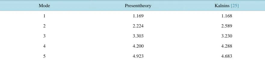
Case 2: clamped spherical shell with φ0 = 30˚
This case was investigated analytically by Kalnins [25] using classical theory and transverse vibration theory. With our theory, we used 8 finite elements to study the spherical shell with the results shown inTable 2. The frequencies we obtained with our model are very comparable to Kalinin’s values.
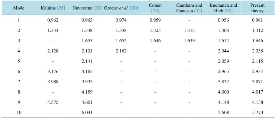
[image:15.595.91.540.650.719.2]Case 3: spherical shell with φ0 = 60˚ under two boundary conditions: clamped, simply supported
Figure 4. Definition of angle φ0.
Table 1.Normalized natural frequencies for 10˚ clamped spherical shell with R/h = 200.
Mode Present theory Sai Ram and Sreedhar babu [23] Narassihan and Alwar [24]
1 1.4861 1.4577 1.4588
2 2.2498 2.2931 2.2999
Table 2. Normalized natural frequencies for 30˚ clamped spherical shell with R/h = 20.
Mode Presenttheory Kalnins [25]
1 1.169 1.168
2 2.224 2.589
3 3.303 3.230
4 4.200 4.288
5 4.923 4.683
Free axisymmetric vibration of the spherical shell in this case was studied by Kalnins [26], Cohen [27], Na-varatna [28], Webster [29], Greene et al. [30], Tessler and Spiridigliozzi [31], Gautham and Ganesan [32] and Buchanan and Rich [33]. In the present investigation, the shell was investigated with 10 elements; the results are given respectively for clamped, simply supported hemispherical shells inTable 3 andTable 4.
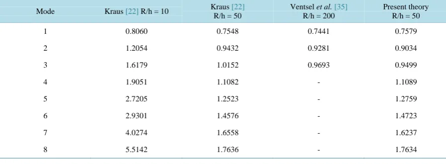
Case 4: spherical shell with φ0 = 90˚
Kraus [22] investigated the case of simply supported spherical shell using a general theory, which included the effects of transverse shear stress and rotational inertia. For cases both with and without these effects, he de-termined the natural frequencies for the shell motion that was independent of θ for circumferential mode number n=0. Tessler and Spiridigliozzi [31], Gautham and Ganesan [34] analyzed the case of clamped he-mispherical shell. Ventsel et al.[35] studied the case of simply supported spherical shell using the boundary elements method for various circumferential mode numbers
(
n=0,n=1,n=2)
. With our model and using 12 finite elements, the natural frequencies were computed for clamped and simply supported shells. The results are shown respectively inTable 5andTable 6.4.1.2. Flutter of Spherical Shells
The problem treated for validation is the flutter boundary of a simply–supported spherical shell subjected to ex-ternal supersonic airflow. As there is no information available for flutter of spherical shells, this case has been compared with simply-supported cone studied by various authors. The conical shell has the following data: Young’s Modulus, E = 6.5 106 lb-in-2, Poisson’s ratio, ν = 0.29, material mass density, ρ = 8.33 10-4 lb-s2-in-4, shell thickness, h = 0.051 in, cone semi-vertex angle α = 5˚. The supersonic airflow has freestream Mach num-ber, M∞ = 3, stagnation temperature, T∞ = 288.15 K. The results are shown in Table 7 where Λ is the dy-namic pressure parameter defined as:
(
)
2 3
2 1
U R
K M
ρ∞ ∞
∞
Λ =
− (69)
where
(
)
3
2 12 1
Et K
ν
=
− is the bending stiffness.
When results are summarized and compared with other finite element and analytical solutions, this method shows good convergence using only 15 elements with small disagreements. It should be noted that the previous analytical methods [13] [15] use Donnel-Mushtari simplified shell theory while [14] uses Novozhilov’s thin shell with the different method of application of finite element solution. On the other hand, a complete form of the linear piston theory is used by [21] as in the present study and the results are very close; but the expression used by Dixon and Hudson [15], Ueda et al. [14] for the piston theory does not have a curvature term which has caused greater differences in the results.
4.2. Flutter Boundary
Table 3. Normalized natural frequencies for 60˚ clamped spherical shell with R/h = 20.
Mode Kalnins [26] Navaratna [28] Webster [29] Tessler and
Spiridigliozzi [31]
Gautham and Ganesan [32]
Buchanan and
Rich [33] Present theory
1 1.006 1.008 1.007 1.000 1.001 1.001 1.031
2 1.391 1.395 1.391 1.368 1.373 1.370 1.496
3 - 1.702 1.700 1.673 1.678 1.675 1.760
4 - 2.126 2.095 - - 2.094 2.089
5 2.375 2.387 2.386 2.260 - 2.256 2.276
6 3.486 3.506 3.851 3.213 - 3.209 3.311
7 3.991 3.996 4.062 3.965 - 3.964 3.775
8 - 4.159 4.151 - - 4.060 4.073
9 4.947 5.001 5.962 4.442 - 4.427 4.826
[image:17.595.85.541.322.524.2]10 - 6.037 6.208 5.773 - 5.740 5.777
Table 4.Normalized natural frequencies for 60˚ simply supported spherical shell with R/h = 20.
Mode Kalnins [26] Navaratna [28] Greene et al.[30] Cohen [27]
Gautham and Ganesan [32]
Buchanan and Rich [33]
Present theory
1 0.962 0.963 0.974 0.959 - 0.956 0.981
2 1.334 1.338 1.338 1.325 1.315 1.308 1.412
3 - 1.653 1.652 1.646 1.639 1.612 1.646
4 2.128 2.131 2.162 - - 2.044 2.038
5 - 2.141 - - - 2.059 2.115
6 3.176 3.185 - - - 2.965 2.934
7 3.988 3.933 - - - 3.837 3.871
8 - 4.159 - - - 4.000 4.017
9 4.575 4.601 - - - 4.148 4.138
10 - 6.031 - - - 5.608 5.773
Table 5.Normalized natural frequencies for 90˚ clamped spherical shell with R/h = 10.
Mode Tessler and Spiridigliozzi [31] Gautham and Ganesan [34] Present theory
1 0.8481 0.8439 0.8327
2 1.2328 1.2317 1.1919
3 1.5902 1.5808 1.5041
4 1.9435 1.9267 1.9161
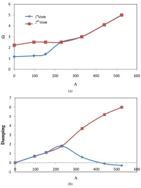
each other in vertical directions (Figure 5). Thus, interaction of two modes occurs. Physically this interaction of the shell modes happens through the effect of the air flow.
A simply supported spherical shell with φ0 = 30˚ is treated here. The complex frequencies only for the first
Table 6.Normalized natural frequencies for 90˚ simply supported spherical shell.
Mode Kraus [22] R/h = 10 Kraus [22]
R/h = 50
Ventsel et al.[35]
R/h = 200
Present theory R/h = 50
1 0.8060 0.7548 0.7441 0.7579
2 1.2054 0.9432 0.9281 0.9034
3 1.6179 1.0152 0.9693 0.9499
4 1.9051 1.1082 - 1.1089
5 2.7205 1.2523 - 1.2759
6 2.9301 1.4576 - 1.4723
7 4.0274 1.6558 - 1.6237
8 5.5142 1.7636 - 1.7634
Table 7. Comparison of critical dynamical pressure parameter (simply supported case).
Present Dixon and Hudson
[15]
Udea et al. [14]
Pidaparti and Yang Henri [21]
Shulman
[13] Bismark-Nasr [17]
520(5)a 590(5) 609(5) 576(5) 669(6) 702(6)
Figure 5. Trajectories of the complex frequencies loci in the complex ω plane during the changing of the dynamic pressure.
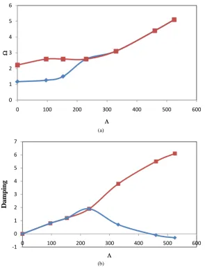
values of dynamic pressure these real parts, representing the oscillation frequency, eventually coalesce into a single mode. Further increasing the dynamic pressure of the flow causes the shell to lose its stability at Λcr = 410. This instability is due to coupled-mode flutter where the imaginary part of complex frequency (representing the damping term of the aeroelastic system) becomes zero for certain critical pressure (Figure 6(b)).
The same behaviour is observed by real and imaginary parts of complex frequencies as the static pressure in-creases (Figure 7) but the onset of flutter is at Λcr = 410 if the freestream static pressure is evaluated using Eq-uation (37). Prediction of the critical freestream static pressure using EqEq-uation (36) provides approximately the same results when evaluating the pressure field using Equation (37). As expected, using the piston theory with the correction term to account for shell curvature produces a better approximation for the pressure loading acting on a curved shell exposed to supersonic flow.
InFigure 8 the onset of flutter for different angles is plotted. By increasing the angle φ0, flutter instability
occurs at lower pressure. This decrease in Λcr with φ0 is attributed to the fact that the natural frequencies
al-ways decrease as the angle φ0 is increased.
(a)
[image:19.595.170.456.81.461.2](b)
Figure 6.(a) Real part and (b) imaginary part of the complex frequencies versus the freestream static pressure parameter; static pressure evaluated by Equation (36).
cylindrical shells.
In order to study the effect of filling ratio,Figure 10 shows the critical value of freestream static pressure for different filling ratios, H/R. Shell geometry and flow parameters are the same as the previous case study with liquid filled density ρf =9.355 × 10⁻⁵lb s2 in-4. It is seen that the value of critical dynamic pressure parameter decreases as the filling ratio increases from a low value. This rapid change in critical dynamic pressure at low filling ratios and its almost steady behaviour at large filling ratios indicates that the fluid near the bottom of the shell is largely influenced by elastic deformation when a shell is subjected to external supersonic flow.
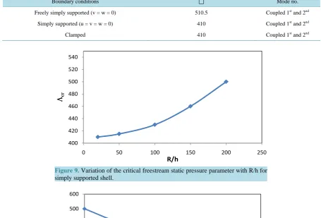
The effect of boundary conditions on the flutter onset is presented inTable 8. It is seen that for freely simply supported ends, v = w = 0, flutter onset occurs at Λ = 510.5 which indicates more flutter resistance compared to simply supported or clamped ends. It is indicated that there is no difference for flutter onset when the shell is either clamped or simply supported. We obtained the same results in the conical shells subjected to supersonic flow.
5. Conclusion
An efficient hybrid finite element method is presented to investigate the aeroelastic stability of an empty or par-tially liquid filled spherical shell subjected to external supersonic flow. Linear shell theory is coupled with first order piston theory to account for aerodynamic pressure. The effect of curvature correction in piston theory was
0 1 2 3 4 5 6
0 100 200 300 400 500 600
Ω
Λ 系列1
系列2
-1 0 1 2 3 4 5 6 7
0 100 200 300 400 500 600
D
a
m
pi
ng
(a)
[image:20.595.167.463.82.468.2](b)
Figure 7.(a) Real part and (b) imaginary part of the complex frequencies versus the freestream static pressure parameter; static pressure evaluated by Equation (37).
Figure 8.Variation of the critical freestream static pressure parameter with an-gle φ0 for simply supported shell.
0 1 2 3 4 5 6
0 100 200 300 400 500 600
Ω
Λ
-1 0 1 2 3 4 5 6 7
0 100 200 300 400 500 600
D
a
m
pi
ng
Λ
-1 0 1 2 3 4 5 6 7
0 100 200 300 400 500 600
D
a
m
pi
ng
[image:20.595.170.458.517.688.2]Table 8. Critical freestream pressure parameter for different boundary conditions.
Boundary conditions Mode no.
Freely simply supported (v = w = 0) 510.5 Coupled 1st and 2nd
Simply supported (u = v = w = 0) 410 Coupled 1st and 2nd
[image:21.595.166.462.378.542.2]Clamped 410 Coupled 1st and 2nd
Figure 9. Variation of the critical freestream static pressure parameter with R/hfor simply supported shell.
Figure 10. Variation of the critical freestream static pressure parameter with R/H for simply supported shell.
analyzed. Fluid structure interaction due to hydrodynamic pressure of internal fluid is also taken into account. The study has been done for shells with various geometries, radius to thickness ratios, filling ratios and boun-dary conditions. In all study cases one type of instability is found; coupled-mode flutter in the first and second mode. Increasing the radius to thickness ratio leads the onset of flutter to occur at higher dynamic pressure. De-creasing the angle φ0 of the spherical shell causes the flutter boundary to occur at lower dynamic pressure. A
lower filling ratio has more flutter resistance than a higher filling ratio. The proposed hybrid finite element for-mulation can give reliable results at less computational cost compared to commercial software since the latter imposes some restrictions when such analysis is done.
References
[1] Bismarck-Nasr, M.N. (1996) Finite Elements in Aeroelasticity of Plates and Shells. Applied Mechanics Reviews Jour-400
420 440 460 480 500 520 540
0 50 100 150 200 250
Λcr
R/h
0 100 200 300 400 500 600
0 0.2 0.4 0.6 0.8 1 1.2 Λcr