Two Methods for Surface/Surface Intersection Problem
Comparative Study
Ramadhan Abdo Musleh Alsaidi
ChinaSchool of Mathematics and Statistics Huazhong University of Science and Technology
ABSTRACT
The determination of the intersection curve between two surfaces may be seen as two different and sequential problems (1) determin-ing initial points of the intersection curve and (2) tracdetermin-ing it from these points. Presented in this paper are: one technique for comput-ing the initial point, and two methods for traccomput-ing the intersection curve of two parametric surfaces. Algorithms, implementation, and illustrative examples will be discussed as well as a comparative analysis of each method.
Keywords:
Surface/surface intersection, B´ezier surface, Continuation method, The Marching Method with Differential Equations
1. INTRODUCTION
For a long time now of computer aided manufacturing [CAM] and computer aided design [CAD], intersection algorithms have always played a central role in making geometric modeling systems work. The first geometric modelers were curve based, and efficient algo-rithms were developed giving satisfactory intersection results. One example of such a system was the AUTOKON system, a com-plete batch oriented CAD/CAM-system for ship building which was developed in Norway in the 1960s. However, when surface and volume based systems were developed, intersection algorithms became more complex.
In curve based systems, the result of an intersection is points or segments of the curves being intersected. Thus, describing the in-tersection is fairly straight forward. In surface based systems the result of an intersection is points, curves, and regions of the sur-faces being intersected[14].
1.1 Motivation
The computation of self-intersection for a patch or inter-section between two patches is an important problem in Computer Aided Geometric Design [CAGD]; and this prob-lem was the main topic of the European project GAIA II [http//www.sintef.no/static/AM/gaiatwo/].
In fact calculation of intersection curves between surfaces can be applied to various fields, such as computational geometry, solid modeling, geometric processing, computer aided design
[CAD], computer aided geometric design [CAGD], manufacturing, numerical-controlled machining, visualization, and robotics. In many applications, there is need to find the curves where two surfaces intersect, for example
—Constructing a contour map to graphically represent a prescribed surface or hyper-surface.
—Computing silhouettes to improve the graphical display of sur-faces.
—Performing Boolean operations on solid bodies. —Constructing smooth blending curves and surfaces.
—Finding offset curves and surfaces, e.g., Numerical-Controlled machining (NC-construction) (Theoretically defined offsets can have self-intersections)[22].
The main goal concerning the surface to surface intersection prob-lem is to develop robust, accurate and fast algorithms for computing the intersection curve between two surfaces, needing the least user intervention.
1.2 Related Work
to the surface-surface intersection problem is a topological and differential-equation method[11]. In this method, the vector field defined as the gradient of the oriented distance function is used to detect critical points in the field such as singularities. Tensorial differential equations are then used to trace intersection segments. Another method that uses unidimensional searches to detect inter-section points was presented by Aomura and Uehara[3]. Surface intersection using parallelism was addressed by Chang et al.[10]. A different approach to higher-dimensional formulation including offsets, equal distance surfaces and variable radius blending sur-faces was discussed by Hoffman[21]. A higher-dimensional formu-lation was also used by Chuang[12] to determine a local and global approximant. Marching methods have been extensively used by re-searchers in this field[11]. The accuracy of marching methods has been improved by proper control of the step size. Singularities were analyzed by Abdel-Malek,K. ,Harn-Jou Yah and Rockwood, A.[1] by locally constructing a second-order approximant to each surface. Parametric surface-surface intersection has also been addressed by Houghton et al.[23] Garrity and Warren[18] and Mullenheim[26]. Singularities along the intersection curve have been identified in the work by Lukacs[27] who used the quadratic of the curves cur-vature to detect any bifurcation points. Eigen values of this system were then studied to determine the form of the matrix, and thefore its behavior at critical points. Most numerical algorithms re-quire the estimation of a starting point on or close to the solution curve. This topic forms the starting point of this paper. In recent years, there have been many studies concerning the determination of the initial points for tracing intersection curves. Cugini et al.[7] introduced the concept of shrinking bounding boxes that cover the total space. Parts of the two surfaces existing in the same bounding box are identified to calculate a starting point. The curve is then traced by introducing one additional constraint as the tangent to an advancing plane. The problem of loop detection was also ad-dressed using relatively simpler algorithm[22, 34]. Although these algorithms may miss intersection components, they are somewhat simpler, more geometric, and in some cases more effective. Muel-lenheim [25] presented an iterative method for calculating a starting point that is close to a solution curve. The starting point has also been computed using lattice and subdivision methods[27]. Con-tinuation methods[2, 31, 21, 16] were recently used to trace the curve and to determine tangents at bifurcation points[1]. Currently, the most widely used surface intersection algorithm is recursive subdivision[9, 10]. In most approaches, the determination of ini-tial points faces the task of solving multivariable polynomial sys-tems. Mrio C. F. and Marcos S. G. T. used the Projected Polyhedral Method to solve the multivariable polynomial systems[17]. Finally, in one of the new studies[8], the authors proposed a new method for computing an equation of a plane curve that is in correspon-dence with the intersection space curve of these two surfaces for very general parameterizations. This paper focuses on the problem of computing the intersection of two parametric surfacesX(u, v)
andY(s, t), since a common representation of surfaces in Solid Modeling and Computer Aided Geometric Design (CAGD) uses parameterized patches.( we address the computation of the intersec-tion curve of two surface patches of bidegree (2,2),i.e., biquadratic patches.).
The rest of this paper is structured as follows. Section 2 we intro-duce and review the problem as well as some basic concepts and terminology to be used throughout the paper. For computing, the initial point of the intersection curves a technique is based on ex-tended Newton Method is presented in section 3. Section 4 present two different techniques for tracing the intersection curves. We ap-ply the two techniques to four representative examples and report
the results in Section 5. Finally, the conclusions and future work are discussed in Section 6.
2. OVERVIEW OF THE PROBLEM AND SOLUTION
Indeed two surfaces of any kind can have one of the following two relationships with each other
—The two surfaces have no points in common. —The two surfaces have a set of points in common.
The first relationship indicates that the two surfaces do not inter-sect. The second relationship is the main interest of this study, be-cause it implies that the two surfaces actually intersect. If the set of points of the intersection of the two surfaces is not empty, then there are two possibilities
—The set contains only one point.
—The set contains more than one point, in which case the intersec-tion could be either a line (a set of lines), or a smooth patch (a set of smooth patches).
In fact the generic algorithm for computing the intersection curve(s), consists of three steps which are:
—Find at least one point on each component of the intersection, —trace the segments of the intersection curve, and
—collect and convert the segments into a format that is suitable for further processing (depending on the application).
2.1 Mathematical Formulation of the Problem
Let two surfaces be X(u, v) =
X1(u, v)
X1(u, v)
X1(u, v)
and
Y(s, t) =
Y1(s, t)
Y2(s, t)
Y3(s, t)
where, X, Y ∈C1[0,1]2.are given, the problem of intersection is solved by computing the set
M=
{(u, v, s, t)∈[0,1]4kF(u, v, s, t) =X(u, v)−Y(s, t) = 0} ⇐⇒
F(u(α), v(α), s(α), t(α)) =
X1(u, v)−Y1(s, t)
X2(u, v)−Y2(s, t)
X3(u, v)−Y3(s, t)
=
f1(u, v, s, t)
f2(u, v, s, t)
f3(u, v, s, t)
=
0 0 0
In the non-degenerate case i.e. the set of intersection points is not empty, the solution manifoldM consists of one or several curves, each fulfilling the condition
F(u(α), v(α), s(α), t(α)) = 0 (1) whereαis any parameter. It can be interpreted as a pair of two curves as:
k1(α) = u(α), v(α)
T
⊆[0,1]2and k
2(α) = s(α), t(α)
T
⊆
[0,1]2
2.2 Basic Concepts and Terminology
In this paper we restrict ourselves to parametric surfaces (including B´ezier surface), which are assumed to be differentiable at any point since the parametric representation is the most used mathematical representation in industry. The parametric surfaces are described by a vector-valued function of two variables
S(u, v) = x(u, v), y(u, v), z(u, v)
whereu, v∈Ω⊂R2 (2)
whereuandvare the surface parameters. Expression 2 is called a parameterization of the surfaceS. At regular points, the partial derivativesSu(u, v) and Sv(u, v) do not vanish simultaneously. These partial derivatives define the unit normal vectorN to the surface atS(u0, v0)as
N = Su×Sv
kSu×Svk
(3)
where × denotes the cross product. A curve in the domain
Ω can be described by means of its parametric representa-tion {u=u(s), v=v(s)} . This expression defines a three-dimensional curve C(s) on the surface S given by C(s) =
S u(s), v(s)
. Applying the chain rule, the tangent vectorC`(w)
of this curve at a pointC(s)becomes
`
C(w) =Su·u`(w) +Sv·`v(w) (4)
In this work the curveC(w)will usually be parameterized by the arc-lengthw. Its geometric interpretation is that a constant stepw traces a constant distance along an arc-length parameterized curve. Since some industrial operations require an uniform parameteriza-tion, this property has several practical applications. For example, in computer controlled milling operations, the curve path followed by the milling machine must be parameterized such that the cutter neither speeds up nor slows down along the path. Consequently, the optimal path is that parameterized by the arc-length.
2.2.1 B´ezier Surfaces. The B´ezier surfaces are widely used in CAD applications. Such parametric surfaces are defined by the fol-lowing expression[22]
S(u, v) =
m
P
i=0 n
P
j=0
Bm
i (u)Bjn(v)·Pij
WherePij are the control points of the surface and Bim(u) , Bn
j(v)
are Bernstein polynomials, defined by
Bm i (u) =
n i
·ui·(1−u)n−i,0≤u≤1e.g. u∈[0,1]
where niis the binomial coefficient which defined as
n i
= n!
i!·(n−i)!
Nonetheless, the Bernstein polynomials have, among others, the following main properties
Bm
i (u)>0, ∀u∈[0,1] m
P
i=0
Bm i (u) = 1
The control points are disposed in a rectangular net ofn+ 1by m+ 1point. This way, the position of a surface point in thexyz space is given by
S(u, v) =
x(u, v)
y(u, v)
z(u, v))
where each coordinate is defined by a polynomial inuandv. The surface degree (and therefore, the degree of the polynomials that describe each coordinate) is given bymandn.
3. FINDING A START POINT INCLUSION
3.1 Tracing a Branch of an Intersection Curve (continuation method)
As mentioned above the calculating surface intersection point means solvingY(s, t) = X(u, v)f or(u, v, s, t)the algorithms introduced here is a kind of marching method which follows the different branches of the solution performed within the parameter space. For each of these methods, it is necessary to obtain appro-priate start points lying within the solution manifold. The curve tracing is initiated at these points.
3.2 Extended Newton Method
In this section, some basic definitions and theorems of a method for determining the roots of an arbitrary system of equation iteratively are given, where the equations can be nonlinear algebraic or transcendental. The number of equations of the system can be greater than, less than or equal to the number of variables. Details of this method can be found in[6].
Let X = [x1, x2, . . . , xk]T be a k-dimensional col-umn vector with components x1, x2, . . . , xk in C and F(X) = [f1(x), f2(x), . . . , fh(x)]T an h-dimensional vec-tor valued function. To deal with the norm of a vecvec-tor, we can choose any one of the norms, for example
kXkp= (Pn i=1|xi|
p
)1p,∀1≤p<∞ and kXk
∞=
max(|x1, . . . , xn|)
We define the Jacobian matrix offw.r.t.xto be theh×kmatrix as
Jf(x) =
∂fi(x)
∂xj
i=1...h,j=1...k
Whenh=kand with the assumption thatdet(J(x))6= 0forx in a closed and bounded setS, we will denote the inverse Jacobian offat xby Jf−1. In this case, Newtons method is a wellknown iterative method for determining the roots of the equationf(x) = 0
. The iteration can be written in the form
xn+1=g(xn), where g(xn) =xn−Jf−1(xn)·f(xn) Unfortunately, hereh6=k, the Jacobian matrix of is not a square matrix. Therefore, it cannot be inverted. Hence, Newtons method fails to apply to such cases. We extend Newtons method such that the extended method can be applied to these cases as well. To get around the problem of a n-square matrix, we will use what we call the pseudo inverse of the Jacobian matrix.
Definition 1
A pseudo inverse of a matrixAis a matrixA⊥
satisfying
AA⊥A=A, A⊥AA⊥=A⊥, (A⊥A)?=A⊥
where(.)?denotes the conjugate transpose of the matrix in case of real coefficient functions, we will use(.)T for (.)?.
Theorem 1
For any matrix A there exists a pseudo inverse matrix A⊥
. Moreover the pseudo inverse is unique.
There are several techniques for obtaining the pseudo inverse of a numerical matrix, for example Hestenes technique or Grevilles technique (see[24]). However, those techniques are pure numerical techniques, i.e., they can only be applied to each individual nu-merical matrix; and we have to take into the account the problems of rounding error, word length, precision of arithmetic, and so on. Moreover, when we use such techniques in our iterative method for determining the roots of a system of equations, we have to apply the approximate process for obtaining the pseudo inverse matrixJ⊥at each iterate
J−(
x(0), x(1), . . . , x(n), . . . ) = J(x)·JT(x)−1
·JT(x) That means that it is time consuming and has accumulated errors. To avoid such problems, we try to find a symbolic formula and use symbolic computation for the method. For example
J+=JT·(J·JT)−1 or J−= (JT·J)−1·JT Lemma 1
For all x, if (J·(x)JT(x)) is nonsingular then J+(x) is the pseudo inverse of matrix J(x).
Proof Lemma 1
The matrixJ+(x)is defined when(J(x)·JT(x))is nonsingular; and it is easy to check thatJ+(x)satisfies the definition 1. Lemma 2
For allx, if(JT(x)·J(x))is nonsingular thenJ−(x)is the pseudo
inverse of matrixJ(x).[13] Lemma 3
For allx, if bothJ+(x)andJ−(x)exist then they are identical.
MatrixJ+(x)orJ−(x)is a matrix of orderk×h. Hence, we can
define the functiongas follows
g(x) =x−J+(x)·f(x)or g(x) =x−J−(x)·f(x)
whereg(x) , xare vectors of the same dimension k and f is defined as equ.1. We find a fixed point of the functiongw.r.t. the initial pointx(0)by the following algorithm
Algorithm 1 (Extended Newton Method).
Input: a functionF :C4 → C3, an initial pointx(0), a measured value (a toleranceε) and a maximum number of iteratesM. Output: A starting point.
Method steps
(1) Let initial number of iteration (L= 1) and
F(u(α), v(α), s(α), t(α)) =
X1(u, v)−Y1(s, t)
X2(u, v)−Y2(s, t)
X3(u, v)−Y3(s, t)
=
f1(u, v, s, t)
f2(u, v, s, t)
f3(u, v, s, t)
(2) Compute Jacobian matrixJatx(0)as:
Jf(x(0)) =
∂fi(x(0))
∂xj
i=1...3,j=1...4
(3) Evaluate a functionFatx(0). (4) Extract new point via [expr]
xnew=x(0)−pinv(J(x(0)))×F(x(0)).
where (pinv) is pseudo inverse. (5) Computet=kxnew−x(0)k. (6) Do testif t≤ε
then Start−point=xnew, exit. else if t>ε and N≤M
set x(0)=x
new, L=L+ 1; goto step2.
else return (f ailure non − convergence try f or new initial point).
4. ALGORITHMS FOR TRACING THE INTERSECTION CURVES
Once the starting point is found, the subsequent points on the in-tersection curve can be traced along the tangent direction. Suppose the parametric coordinates of the starting pointqare(u0, v0)and
(s0, t0).The constraint functionH(q)is defined by
F(q) =
X1(u0, v0)−Y1(s0, t0)
X2(u0, v0)−Y2(s0, t0)
X3(u0, v0)−Y3(s0, t0)
(5)
The Jacobian of the constraint functionF(q)for a certain configu-rationqis the3×4matrix as:
Jf(q) =
∂f i(q)
∂xj
i=1...3,j=1...4
Here, the tangent vector λ to the set defined by H(q) = 0 is uniquely defined by
Jf(q)·λ= 0 (6)
kλk2= 1 (normalization). (7)
det
Jf(q) λT
>0 (8)
Where Equations 6,7 and 8 were set forth to define a unique tangent in the Predictor-Corrector method [17]. Combining equation 5 and equation 6 yields a system of four equations in four variables, such that the Newton-Raphson iteration method can be used to calculate the new pointx. By setting the new point as the current point, the tracing is continued until one of three cases occurs
(1) the boundary is reached, (2) returning to the starting point, or (3) reaches to the non-convergence point.
The Complete Algorithm
(1) Find an inclusion of one start point of an intersection curve denote byq.
(2) Solve equation 6 then set ite.
(3) Using relationxnew =q±(e×d)to compute a new initial guess point.(wheredis the desire distance)
4.1 The Marching Method with Differential Equations
LetF(u, v) andG(s, t)be two surfaces whose unit normal vec-tors at a point on the intersection curveC(w)betweenF(u, v)and G(s, t)areN1andN2respectively.
N1=kFFuu××FFvvk, N2=
Gs×Gt
kGs×Gtk
Once the initial points of the intersection curves are obtained, each curveC(w) ,parameterized by the arc lengthw, is traced using the Marching Method proposed by [9]. The marching direction is given by the tangent vector ofC(w), which is perpendicular to the normal vector of both surfaces at the given intersection point
`
C=dCdw= N1×N2
|N1×N2|
Applying the chain rule, we obtain the unit tangent vectorT1(w) (T2(w)resp.) to the curveC(w)considered as belonging to the surfaceF(Gresp.) is given by
dC dw =
du dw·Fu+
dv dw·Fv. dC
dw = ds dw·Gs+
dt dw·Gt.
BecauseT1andN2are orthogonal and so areT2andN1we have
∂F ∂u ·N2
· du dw + ∂F ∂v ·N2
· dv dw
= 0,
∂G ∂s ·N1
· ds dw + ∂G ∂t ·N1
· dt dw = 0 (9)
On the other hand, since the curveC(w)belongs to bothFandG, we have E1 du dw 2
+ 2P1 du dw dv dw
+Q1
dv dw
2
= 1,
E2
ds dw
2
+ 2P2 ds dw dt dw
+Q2 dt dw 2 = 1 (10)
where E,P and Q are the coefficients of the First Fundamental Form of the surface given by:
E1=Fu·Fu, P1=Fu·Fv, Q1=Fv·Fv E2=Gs·Gs, P2=Gs·Gt, Q2=Gt·Gt Solving equation 9 and 10 for du
dw, dv dw, ds dw and dt
dw we obtain
du dw=±
∂F ∂v ·N2
q
E1 ∂F∂v ·N2 2
−2P1 ∂F∂v ·N2 ∂F
∂u ·N2
+Q1 ∂F∂u·N2 2
dv dw=∓
∂F ∂u·N2
q
E1 ∂F∂v ·N2 2
−2P1 ∂F∂v ·N2 ∂F
∂u ·N2
+Q1 ∂F∂u·N2 2
ds dw=±
∂G ∂t ·N1
q
E2 ∂G∂t ·N1 2
−2P2 ∂G∂t ·N1 ∂G
∂s ·N1
+Q2 ∂G∂s ·N1 2
dt dw=∓
∂G ∂s ·N1
q
E2 ∂G∂t ·N1 2
−2P2 ∂G∂t ·N1 ∂G
∂s ·N1
+Q2 ∂G∂s ·N1 2 (11)
which together with an initial point of the intersection curve(u(0), v(0), s(0), t(0)) = (u0, v0, s0, t0)constitutes an ini-tial value problem for this system of four explicit first-order ordi-nary differential equations. The signs±and∓in 11 mean that there are two arcs of curve starting at(u0, v0, s0, t0)associated with the
two possible opposite directions of the tangent vectorsT1(w)and
T2(w)[17]. Above are the equations from which the points of the intersection curves may be successively determined using a numer-ical integration method for the problem of the initial value with the given system of ordinary differential equations of 11 [5] Hu et al. did not explain which method was used to integrate the ordinary differential equations, as a first implementation we decided to use the4thorder Runge-Kutta Method to accomplish this task. So, the Marching Algorithm has the following steps:
Step1: Obtaining initial points for the algorithm, which means at least one point for each intersection curve. This is done using the procedures presented in the previous sections.
Step2: For each of these points, are obtained the derived equations of the surface parameters with respect to the arc length of the inter-section curve using Eq.11.
Step3: Integrate this system of ordinary differential equations using a numerical method (4thorder Runge-Kutta, for instance), provid-ing this way the next point of the intersection curve.
Steps 2 and 3 are repeated until the traced curve reaches a turning point or an initial border points (previously determined).
5. SOME ILLUSTRATIVE EXAMPLES
5.1 Example
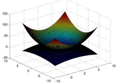
To illustrate the determination of surfaces intersection using the continuation method that outlined above. Consider the two surfaces
S1(u, v) =
u v u2+v2
,S2(s, t) =
s t
9−(s2+5t2)
where the two surfaces are shown in figure 1. Firstly to
demon-Fig. 1. Two parametric surfaces intersecting
[image:5.595.335.540.430.575.2]Table 1. list some of intersection points for example 5.1
kthPoint Coordinates kthPoint Coordinates
[image:6.595.348.525.222.351.2]0 (1.9365,1.9365,1.9365,1.9365) 240 (-1.9278,1.9451,-1.9278,1.9451) 4 (1.7811,2.0803,1.7811,2.0803) 276 (-1.9330,1.9400,-1.9330,1.9400) 20 (0.8477,2.6041,0.8477,2.6041) 301 (-1.9347,1.9383,-1.9347,1.9383) 33 (0.1167,2.7361,0.1167,2.7361) 367 (-1.9362,1.9368,-1.9362,1.9368) 42 (0.48420.1249,0.4910,0.1454) 89 (0.3823,0.1552,0.3865,0.1651) 45 (0.4499,0.1324,0.4552,0.1487) 49 (0.4205,0.1410,0.4250,0.1542)
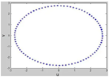
Fig. 2. The result curve of intersection on theu−vspace in Ex. 5.1
5.2 Example
Given two Bezier surfaces(S1and S2)have the control points as:
S1(u, v) =
(17,0,35) (35,15,34) (1,0,107) (3
8, 4 9,
2 3) (
2 3,
3 4,
1 3) (
6 7,
3 8,
5 7)
(1 5,
6 7,
4 7) (
3 4,
7 8,
3 4) (
7 8,
7 9,
5 8)
and
S2(s, t) =
(27,17,25) (35,101,23) (1,0,45) (3
8, 4 9,
2 3) (
1 3,
1 2,1) (
5 7,
3 8,
2 7)
(1 5,
6 7,
3 7) (
3 4,
7 8,
5 8) (
7 8,
4 7,
1 2)
The two Bezier surfaces are shown in Figure3. The initial guess
Fig. 3. Two quadratic Bezier surfaces.
is specified asx0 = (0.99940.25010.99940.2502). At the end of the four iterations the starting point on the curve is computed
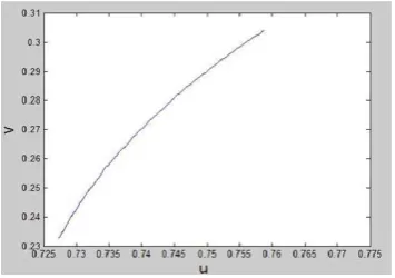
[image:6.595.65.260.378.468.2]asq = (0.72740.23270.73490.2990). The resulting intersection curve using the continuation method after compute 200 points at both sides of start point are shown in Figure4. We list some of
Fig. 4. The result curve of intersection two Bezier surfaces on theu, v
space in Ex. 5.2.
points as follows.
5.3 Example
We will use the two surfaces in example (5.1 ) but here we use the Marching Method with Differential Equations the result of inter-section curve compute100points and choosed = 0.2are shown in figure 5. We list some of points as follows.
[image:6.595.85.262.502.626.2] [image:6.595.347.526.513.640.2]Table 2. List some of intersection points for example 5.2
kth point Coordinates kth point Coordinates
0 (0.7274,0.2327,0.7849,0.2990) 57 (0.3939,0.1505,0.3981,0.1613) 5 (0.6506,0.4785,0.7954,0.5829) 64 (0.3862,0.1536,0.3904,0.1637) 15 (0.5868,0.5138,0.7475,0.6408) 77 (0.3827,0.1550,0.3870,0.1649) 25 (0.5839,0.5149,0.7450,0.6428) 80 (0.3825,0.1551,0.3868,0.1650) 33 (0.7031,0.1782,0.7436,0.2362) 81 (0.3825,0.1551,0.3867,0.1650) 78 (-1.3338,2.3919,-1.3338,2.3919) 409 (-1.9364,1.9366,-1.9364,1.9366) 100 (-1.6064,2.2180,-1.6064,2.2180) 420 (-1.9364,1.9366,-1.9364,1.9366) 130 (-1.7882,2.0742,-1.7882,2.0742) 433 (-1.9364,1.9366,-1.9364,1.9366) 200 (-1.9123,1.9604,-1.9123,1.9604) 450 (-1.9365,1.9365,-1.9365,1.9365)
Table 3. List some of intersection points for example 5.3
kth point Coordinates kth point Coordinates
0 (1.9365,1.9365,1.9365,1.9365) 54 (-2.7343,-0.1545,-2.7343, 0.1545) 7 (2.5752,0.9319,2.5752, 0.9319) 60 (-2.5415,1.0202,-2.5415,1.0202) 15 (2.6621,-0.6430,2.662,-0.6430) 67 (-1.7174 ,2.1332 ,-1.7174,2.1332) 23 (1.8658,-2.0047,1.8658,-2.0047) 73 (-0.6501,2.6603,-0.6501,2.6603) 33 (0.0527,-2.7381,0.0527,-2.7381) 80 (0.7345,2.6383,0.7345,2.6383) 37 (-0.7380,-2.6373,-0.7380,-2.6373) 89 (2.1934,1.6399,2.19341.6399) 40 (-1.2936,-2.4139,-1.2936-2.4139) 93 (2.5727,0.9388,2.5727,0.9388) 43 (-1.7873,-2.0750,-1.7873,-2.0750) 97 (2.7341,0.1581,2.7341,0.1581) 50 (-2.5739,-0.9353,-2.5739 ,0.9353) 100 (2.7031,-0.4399 ,2.7031,-0.4399)
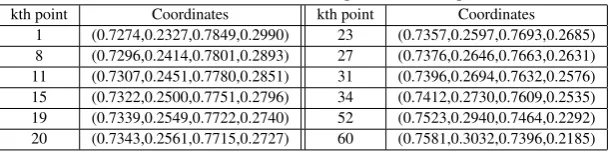
5.4 Example
[image:7.595.85.263.394.519.2]We will use the two surfaces in example (5.2) but here we use the Marching Method with Differential Equations the results of inter-section curve are shown in figure 6. We can drive60points using
Fig. 6. Result curve obtained by using Marching Method for Bezier sur-faces.
the Marching Method with Differential Equations, and we list some of them as follows.
6. CONCLUSION
I presented two different algorithms for computing the intersection curve between two parametric surfaces. I implemented the meth-ods using Matlab software and applied them to many test cases include Bezier surface. The continuation method was able to deal with all test cases. It may produce subsequent points on the inter-section curve along the tangent direction but not all the points. We have noticed using this practical method that the processing time
taking is short which make it relatively fast meanwhile it keeps its accuracy rate relatively high. After experimenting with Marching Method with Differential Equations we arrived at the conclusion this method is very general, it can be applied to any pair of para-metric surfaces and it has shown a very good performance in the examples described in this paper but it takes longer time specially in Bezier surfaces and the accuracy is not very sufficient, so these methods for Bezier surface have not yet been developed enough to come up with practical results and warrant further research.
7. REFERENCES
[1] Karim Abdel-Malek and Harn-Jou Yeh. Determining inter-section curves between surfaces of two solids. Computer-Aided Design, 28(6):539–549, 1996.
[2] Eugene L Allgower and Kurt Georg.Numerical continuation methods, volume 13. Springer-Verlag Berlin, 1990.
[3] S. Aomura and T. Uehara. Intersection of arbitrary sur-faces.Journal of the Japan Society of Precision Engineering, 57(9):1673–1679, 1991.
[4] Chandrajit L Bajaj, Christoph M Hoffmann, Robert E Lynch, and JEH Hopcroft. Tracing surface intersections.Computer aided geometric design, 5(4):285–307, 1988.
[5] Robert E Barnhill.Geometry processing for design and man-ufacturing. SIAM, 1992.
[6] Thomas L Boullion and Patrick L Odell.Generalized inverse matrices. Wiley-interscience New York, 1971.
[7] Heiko B¨urger and Robert Schaback. A parallel multistage method for surface/surface intersection.Computer aided geo-metric design, 10(3):277–291, 1993.
[8] Laurent Bus´e and Thang Luu Ba. The surface/surface inter-section problem by means of matrix based representations. Computer Aided Geometric Design, 29(8):579–598, 2012. [9] Vijaya Chandru, Debasish Dutta, and Christoph M.
!
Table 4. List some of intersection points for example 5.4
kth point Coordinates kth point Coordinates
1 (0.7274,0.2327,0.7849,0.2990) 23 (0.7357,0.2597,0.7693,0.2685) 8 (0.7296,0.2414,0.7801,0.2893) 27 (0.7376,0.2646,0.7663,0.2631) 11 (0.7307,0.2451,0.7780,0.2851) 31 (0.7396,0.2694,0.7632,0.2576) 15 (0.7322,0.2500,0.7751,0.2796) 34 (0.7412,0.2730,0.7609,0.2535) 19 (0.7339,0.2549,0.7722,0.2740) 52 (0.7523,0.2940,0.7464,0.2292) 20 (0.7343,0.2561,0.7715,0.2727) 60 (0.7581,0.3032,0.7396,0.2185)
[10] Long Chyr Chang, Wolfgang W Bein, and Edward Angel. Surface intersection using parallelism.Computer aided geo-metric design, 11(1):39–69, 1994.
[11] Koun-Ping Cheng. Using plane vector fields to obtain all the intersection curves of two general surfaces. InTheory and practice of Geometric Modeling, pages 187–204. Springer, 1989.
[12] Jung-Hong Chuang and Christoph M Hoffmann. On local im-plicit approximation and its applications.ACM Transactions on Graphics (TOG), 8(4):298–324, 1989.
[13] Qiulin Ding and Beaumont John Davies.Surface engineering geometry for computer-aided design and manufacture. Pren-tice Hall Professional Technical Reference, 1988.
[14] Tor Dokken. Aspects of intersection algorithms and approxi-mation.Doctor thesis, 1997.
[15] Rida T Farouki. The characterization of parametric surface sections.Computer Vision, Graphics, and Image Processing, 33(2):209–236, 1986.
[16] M´ario Carneiro Faustini and Marcos Sales Guerra Tsuzuki. Algorithm to determine the intersection curves between bezier surfaces by the solution of multivariable polynomial system and the differential marching method.Journal of the Brazilian Society of Mechanical Sciences, 22(2):259–271, 2000.
[17] Akemi G´alvez, Jaime Puig-Pey, and Andr´es Iglesias. A dif-ferential method for parametric surface intersection. In Com-putational Science and Its Applications–ICCSA 2004, pages 651–660. Springer, 2004.
[18] Thomas Garrity and Joe Warren. On computing the intersec-tion of a pair of algebraic surfaces.Computer Aided Geomet-ric Design, 6(2):137–153, 1989.
[19] Michael Gleicher and Michael Kass. An interval refinement technique for surface intersection. InProceedings of the con-ference on Graphics interface’92, pages 242–249. Morgan Kaufmann Publishers Inc., 1992.
[20] Christoph M Hoffmann.Geometric and solid modeling: an introduction. Morgan Kaufmann Publishers Inc., 1989. [21] Christoph M Hoffmann. A dimensionality paradigm for
surface interrogations.Computer Aided Geometric Design, 7(6):517–532, 1990.
[22] Josef Hoschek, Dieter Lasser, and Larry L Schumaker. Fun-damentals of computer aided geometric design. AK Peters, Ltd., 1993.
[23] Elizabeth G Houghton, Robert F Emnett, James D Factor, and Chaman L Sabharwal. Implementation of a divide-and-conquer method for intersection of parametric surfaces. Com-puter Aided Geometric Design, 2(1):173–183, 1985.
[24] SM Hu, JG Sun, TG Jin, and GZ Wang. Computing the pa-rameters of points on nurbs curves and surfaces via moving affine frame method.Journal of Software, 11(1):49–53, 2000. [25] George A Kriezis, Nicholas M Patrikalakis, and F-E Wolter. Topological and differential-equation methods for surface in-tersections.Computer-Aided Design, 24(1):41–55, 1992. [26] George A Kriezis, Prakash V Prakash, and Nicholas M
Patrikalakis. Method for intersecting algebraic surfaces with rational polynomial patches. Computer-Aided Design, 22(10):645–654, 1990.
[27] Gabor Lukacs. Simple singularities in surface-surface inter-sections. InINSTITUTE OF MATHEMATICS AND ITS AP-PLICATIONS CONFERENCE SERIES, volume 48, pages 213–213. OXFORD UNIVERSITY PRESS, 1994.
[28] Robert P Markot and Robert L Magedson. Procedural method for evaluating the intersection curves of two parametric sur-faces.Computer-Aided Design, 23(6):395–404, 1991. [29] Yves de Montaudouin, Wayne Tiller, and Havard Vold.
Applications of power series in computational geometry. Computer-Aided Design, 18(10):514–524, 1986.
[30] Michael J Pratt and AD Geisow. Surface/surface intersection problems.The mathematics of surfaces, 6:117–142, 1986. [31] Rizzi C Radi S. A system for parametric surface
intersec-tion. InINSTITUTE OF MATHEMATICS AND ITS APPLI-CATIONS CONFERENCE SERIES, volume 48, pages 231– 231. OXFORD UNIVERSITY PRESS, 1994.
[32] Jaroslaw R Rossignac and Aristides AG Requicha. Piecewise-circular curves for geometric modeling.IBM Journal of Re-search and Development, 31(3):296–313, 1987.
[33] Thomas W Sederberg. Planar piecewise algebraic curves. Computer Aided Geometric Design, 1(3):241–255, 1984. [34] Jianrong Tan, Jianmin Zheng, and Qunsheng Peng. A
uni-fied algorithm for finding the intersection curve of surfaces. Journal of Computer Science and Technology, 9(2):107–116, 1994.