Modelling of LFM Spectrum as Rectangle using Steepest
Descent Method
A.NagaJyothi
Research ScholarDepartment of Electronics and Communication Engineering
Andhra University college of Engineering (A), Visakhapatnam
K.Raja Rajeswari
ProfessorDepartment of Electronics and Communication Engineering
Andhra University college of Engineering (A), Visakhapatnam
ABSTRACT
The chirp or LFM waveform has superior performance in radars since they can be easily processed and generated. The amount of compression in pulse compression radar is determined by time-bandwidth product. The LFM waveform exhibits very high time-bandwidth product. The transform of this LFM waveform is flat over its range of frequencies. The signal spectrum will become fairly rectangular if bandwidth product is increased. The bigger the time-bandwidth product the higher is the robustness of radar transmitter.
The focus of this paper is on steepest descent method which when applied to the LFM wave form gets the signal spectrum as a rectangle i.e totally flat over its range of frequencies. By using this method a ideal rectangle spectrum is achieved, which utilizes the total pulse and offers an optimal spectral density. This steepest descent approximated LFM waveform offer high resolution on the time axis and is therefore best suited for ranging.
Keywords
Linear Frequency Modulation(LFM), Time-bandwidth product(BT), Steepest descent method, Spectral amplitude, Fourier Transform, Over sampling factor(k) .
1.
INTRODUCTION
One of the fundamental and important issue in designing a good radar is its ability to differentiate two targets that are located at very long range and separation between them are very small. A radar transmits a long pulse with high energy to detect small targets, which in turn degrades range resolution. A short pulse is required to maintain range resolution. Pulse compression is a technique which allows the radar to achieve the range resolution of short pulse and energy of the long pulse simultaneously [1,2,3] .A simple pulse will be having two parameters one is the amplitude A and other is duration τ. The range resolution ΔR is given by equation 1.
2 / τ c = R
Δ . (1)
It can be clearly seen that range resolution is directly proportional to τ; so better resolution required shorter pulse. The energy in the pulse is given by equation 2
τ A =
E 2 . (2)
Where energy is also proportional to τ; so when the energy is high the detection performance is improved and range resolution is improved by short pulse [3,4,5]. The pulse compression waveform has a BT product much greater than one. A radar transmits a waveform which may defined as
)] t ( θ + ) t ( ω sin[ ) t ( A = ) t (
x . (3)
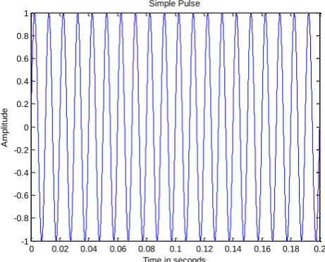
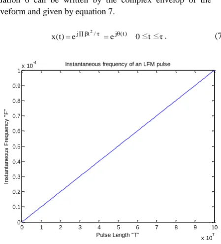
The ω in the above said equation 3 is the radio frequency in radians per second. A(t) represents amplitude modulation of radio frequency carrier . The term θ(t) represents phase or frequency modulation of the carrier signal and it can be zero, non zero or nontrivial function. Commonly used waveforms in pulsed radar are simple pulse, frequency coded pulses and phase coded pulses. Fig. 1(a) is an example of simple pulse of constant amplitude burst signal at the radio frequency. Fig. 1(b) is a LFM waveform and here the frequency increases linearly w.r.t the time. Fig. 1(c) is an example of binary phase-coded waveform. In this θ(t) varies in between the zeros and π at different time within the pulse.
Fig. 1(a).Simple pulsed waveform
0 0.02 0.04 0.06 0.08 0.1 0.12 0.14 0.16 0.18 0.2 -1
-0.8 -0.6 -0.4 -0.2 0 0.2 0.4 0.6 0.8 1
Time in seconds
A
m
p
lit
u
d
e
[image:1.595.328.559.477.663.2].
Fig. 1(b). Linear Frequency Modulation(LFM)
Fig. 1(c). Binary phase coded waveform
The real value of the equation 1 can be written by complex envelope of the waveform
)] ( [ ) ( )
(t Atej wt t
x
. (4)
It can be further given as considering complex envelope of the waveform after demodulation and given by x(t)
) t ( θ j
e ) t ( A = ) t (
x . (5)
The LFM waveform has superior performance in radar since they can be easily processed and generated. This paper has been prepared in the following manner: linear frequency modulation, effects of BT product on the LFM spectrum, the method of steepest descent, results, and conclusion.
2.
Linear Frequency Modulation
The LFM waveform is mostly discussed in literature and extensively used in practice [3,4,9]. A LFM modulation wave can be given by
τ ≤ t ≤ 0 ) t τ β ∏ cos( = ) t (
x 2 . (6)
Where β is bandwidth =1/τ hertz. The real value of the equation 6 can be written by the complex envelop of the waveform and given by equation 7.
τ
≤
t
≤
0 e = e = ) t (
[image:2.595.59.275.76.516.2]x j∏βt2/τ jθ(t) . (7)
Fig. 2. Instantaneous frequency of LFM waveform The derivative of the phase function w.r.t. time gives instantaneous frequency:
dt ) θ ( d ∏ 2
1 = ) t (
F . (8)
Instantaneous frequency sweeps linearly across the total bandwidth of β Hz during the pulse duration τ seconds as shown in Fig. 2. If β is positive, the pulse may be called as upchirp and if β is negative it is called as downchirp.
2.1
Effects of BT Product on LFM
Spectrum
The LFM waveform exhibits an important property of possessing high BT product [4,6,3]. The transform of this waveform is flat over its range of frequencies. If the BT product of the LFM waveform increases , the signal spectrum will become more rectangular in shape. As the waveform spreads the energy uniformly across the spectrum this seems naturally reasonable to consider the spectrum as optimal spectrum .The spectrum of LFM chirps which are generated using MATLAB are shown in this paper. In all their cases, the duration of the pulse is considered to be 1μs. TABLE1 shows different BT product.
TABLE. 1.Different BT which are considered in this paper.
S.No Pulse Length(τ) in μs
Bandwidth(β) in MHz
BT Product
1 1 5 5
2 1 10 10
3 1 50 150
4 1 100 200
0 0.1 0.2 0.3 0.4 0.5 0.6 0.7 0.8 0.9 1
x 10-4 -0.8
-0.6 -0.4 -0.2 0 0.2 0.4 0.6 0.8
Time in u sec
A
m
p
lit
u
d
e
Real part of chirp signal
0 5 10 15 20 25 30 35
-1 -0.8 -0.6 -0.4 -0.2 0 0.2 0.4 0.6 0.8 1
phase coded signal of length N=11
time
a
m
p
li
tu
d
e
0 1 2 3 4 5 6 7 8 9 10
x 107 0
0.1 0.2 0.3 0.4 0.5 0.6 0.7 0.8 0.9
1x 10
-4
Pulse Length "T"
In
s
ta
n
ta
n
e
o
u
s
Fr
e
q
u
e
n
c
y
"
F"
[image:2.595.326.551.112.360.2]By observing the Fig. 3 and Fig. 4 one may conclude that for BT=5 have a spectrum which is very poorly approximated to a rectangular shape. If BT is increased it gives more rectangular spectral magnitude. A BT product of 100 or above is considered to model the LFM spectral as a rectangular shape in practice. Here for all the cases shown in TABLE.1 the amplitude of the spectrum is considered equal and the proof for same is given in section 3.1.
Fig.3. Spectrum of LFM waveform for BT=10
Fig. 4. Spectrum of LFM waveform for BT=100 .
Fig.5. Spectrum of LFM waveform for different BT
[image:3.595.67.284.174.357.2]Fig.5 shows a comparison of four chirps with different BT products. Here we can conclude that higher the BT it takes the rectangular shape .LFM waveform exhibits an important property of possessing high BT product [4,6,3].
3.
The Method of Steepest Descend
The Fourier transform of equation 7 derived by [7,8] is complex due to sine integral Si(β) function. A very simple and useful approximation can be given by using the method of steepest descent which is an advanced technique in Fourier analysis. This method is useful in evaluating the integrals which will be having highly oscillatory integrands; therefore this is particularly applied well to Fourier transforms. equation 7 can be represented in terms of amplitude and phase as
)] t ( θ j exp[ ) t ( A = ) t (
x . (9)
Fourier transform of above equation can be written as
∫ ∞
∞
-dt t ω j -e ) t ( θ j e ) t ( A = ) ω (
X . (10)
dt
∫ ∞
∞
] t ω -) t ( θ [ j e ) t ( A = ) ω ( X
- . (11)
∫ ∞
∞
-) t , θ ( j e ) t ( A = ) ω (
X . (12)
Where
otherwise
0
/2 t /2 1 ) (
t A
The Fourier transform is known for many signals having relatively simple phase function θ(t).Defining a point in the integral as a value (t=t0) such that Φ`(t0,ω) = 0.That is the first
derivate in the above integral is 0. The term X(ω) can be rewritten as [8]
) ω , t ( θ j 0 0
0 e ) t ( x ) ω , t ( ' ' φ 2
∏ -= ) ω (
X . (13)
Where Φ``(t,ω) is second derivate of Φ(t,ω).
The method of steepest descent can be applied to estimate the spectrum of the LFM waveform. The LFM waveform can be defined by
2
t α
e ) t ( A = ) t (
x . (14)
where α = π*β/τ,Now substituting value of α in equation 14 we get
∫ ∞
∞
-) t ω -2 t α ( j e ) t ( x = ) ω (
X . (15)
Integrand phase Φ(t,ω) and its derivative are given as
t t
t
(, ) 2 . (16)
'(t, )2 t . (17)
2 ) , ( '
' t t
. (18)
Now by setting Φ``(t,ω)=0 and solving with respect t0 we get
-0.50 -0.4 -0.3 -0.2 -0.1 0 0.1 0.2 0.3 0.4 0.5
0.2 0.4 0.6 0.8 1 1.2 1.4
Normalized Frequency (cycles)
A
m
p
lit
u
d
e
Spectrum of LFM BT=5
BT=5
-0.50 -0.4 -0.3 -0.2 -0.1 0 0.1 0.2 0.3 0.4 0.5 0.2
0.4 0.6 0.8 1 1.2 1.4
Normalized Frequency (cycles)
A
m
p
lit
u
d
e
Spectrum of LFM BT=100
BT=100
-0.50 -0.4 -0.3 -0.2 -0.1 0 0.1 0.2 0.3 0.4 0.5 0.5
1 1.5
Normalized Frequency (cycles)
A
m
p
lit
u
d
e
Spectrum of LFM with different BT
[image:3.595.54.278.176.765.2] [image:3.595.316.498.298.431.2]value of t0 where (t=t0) and Φ`(t0,ω) = 0
Then t0 = ω/2α
Now inserting the above t0 value in equation (13) we get
) ω , 0 t ( φ j e ) 0 t ( X ) ω , 0 t ( ' ' φ 2 ∏ -α ) ω (
X . (19)
) ) α 2 ω ( ω -2 ) α 2 ω ( α ( j e ) α 2 ω ( A ) α 2 ( 2 ∏ -= ) ω (
X . (20)
α 4 / 2 ω j e ) α 2 ω ( A α 4 ∏ j = ) ω (
X . (21)
Now the signal envelope A(t), the term (ω/2α) becomes (using α=πβ/τ)
otherwise 0 /2 /2 1 2 A . (22)
otherwise 0 ) 2 / ( 2 ) 2 / ( 2 1
2
A . (23)
3.1
Spectral Amplitudes of Four Chirps
Here is the proof for considering equal amplitude of the four chirps. Here the bandwidth of each and every chirp differs; therefore the sampling rate T for each of the chirp is also different. The sampling rates and the corresponding sampling intervals of the chirps are given by equation 9
n k n T n k sn F ⇒ 1
. (24)
Each of the pulse shares 1μs and bandwidth varies so the samples in of the each pulse are also different and proportional to bandwidth β:
n τβ k = sn F τ = n T τ = n
N . (25)
Bandwidth of each signal can be computed in frequency units. Individual bandwidths are given by βn Hz and the spectrum
normally looks like a rectangular function with the limits - βn
Hz to +βn Hz. Digitizing these we get
n T ω = n
ω . (26)
Combining equation 24 and equation 26 we can get
k n k n n T n n ∏ 1 ∏ 2 ∏
2
. (27)
Note: Cutoff frequency is depending on Π and k and same for all of the four chirps. That is the reason why their DFT’s for all the four chirps have same nominal cutoff frequencies, when we plot all together despite of different bandwidths. Now considering the energy in each chirp we get
∑1 0 2 ] [ N
m xm Nn k n E
. (28)
From Parseval’s theorem we can express energy in terms of signal spectrum as
n
d n X
E
2 ∫ ∏ ∏ ( ) ∏ 2 1
. (29)
Now considering equation 25, equation 27 and Steepest descent approximation X(ω) we can say that it is an rectangular function with an amplitude as given below.
2 1 ∫ / ∏ / ∏ 2 ∏ 2 1 n A k n d k
k nA
n k
E . (30)
k n
A . (31)
Since all the four chirps have same k,τ and the time-domain amplitude considered to be 1 same as in Steepest descent method. Now with this we can justify that the individual spectra will have amplitudes proportional to the square root of their individual BT product , so therefore to model the spectrum as rectangle it is necessary to normalize all he spectrum w.r.t square root of BT product which will be convenient for plotting.
4.
Results
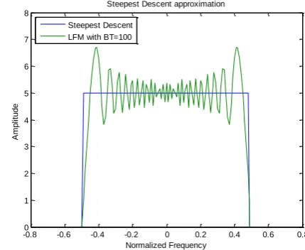
[image:4.595.326.541.396.572.2]Using method of the steepest descent approximation X(ω) is approximately a rectangle function of an amplitude A which is proportional to square root of BT product and k in the frequency intervals (+β/2 , -β/2). In the Fig.6 comparison of LFM spectrum with βT = 100 and X(ω) by using method of the steepest descent is given .It is observed that X(w) is constant over the range (+β/2 , -β/2) and is zero outside the range.
Fig. 6. Comparison of Steepest descent method and LFM waveform with BT=100
In order to have the spectrum occupied most of the plot area, the data is oversampled by a factor of k=1.2 (which is nearly 20%) in each of the case to make the spectral details clearer. In this paper it is shown that the range over which the instantaneous frequency F of the LFM pulse sweeps linearly across the total bandwidth of β Hz during the pulse duration τ, is consistent with the increasing rectangular shape in the frequency domain. By considering this method a ideal rectangular spectrum is achieved which uses the total pulse and offers an optimal spectrum.
5.
Conclusions
This paper gives a detailed description of LFM waveform spectrum. The important characteristics of LFM waveform comprise linear frequency ramp, flat topped rectangle
-0.80 -0.6 -0.4 -0.2 0 0.2 0.4 0.6 0.8
1 2 3 4 5 6 7 8 Normalized Frequency A m p lit u d e
Steepest Descent approximation Steepest Descent
spectrum. Here it is clearly shown that the LFM waveform with a BT product of 5 has a spectrum which is an very poor approximation to a rectangle spectrum. The BT product of 100 gives a good approximation to a rectangular spectrum. In order to model the LFM waveform spectrum as a rectangle usually BT product of 100 or above is considered.
The steepest descent method can be applied to estimate LFM waveform spectrum. X(ω) is constant over the range of frequencies from ±β/2 hertz, and zero outside this range. This is naturally satisfying, since this is exactly the range of frequencies over which the instantaneous frequency of the LFM waveform sweeps, and is consistent with the rectangular shape of the actual spectrum observed in Fig.5 as the BT product increases. The steepest descent method result gives an approximation of the phase of the spectrum which is like the phase of the LFM waveform.
6.
ACKNOWLEDGMENTS
This work is being supported by Ministry of Science & Technology, Department of Science & Technology (DST), New Delhi, India, under Women Scientist Scheme (WOS-A) WOS-A/ET-12/2010 with the Grant No: 100/ (IFD)/8450/2010-11,Dated 15/11/2010.
7.
REFERENCES
[1] Levanon. N, mozeson Radar Signal, 2004. [2] Levanon.N, Radar Prirzciples Wiley, New
York, 1988.
[3] Bassem r. Mahafza, Radar systems analysis and design
using Matlab, Chapman & Hall,CRC, 2000. [4] M.A.Richards, Fundamentals of Radar Signal
Processing, McGraw-Hill, 2005.
[5] Skolnik.M, Radar Handbook, 3rd.ed., McGraw-Hill, New York, 2005.
[6] Y. K. Chan, M. Y. Chua, and V. C. Koo, Sidelobes Reduction Using Simple Two and Tri-Stages Non Linear Frequency Modulation (NLFM), Progress In Electromagnetics Research, PIER98,2009.
[7] David Brandwood, Fourier Transforms in Radar and Signal Processing, Artech House,Boston , London,2003
[8] M.Born, E. Wolf, Principles of Optics,1983. [9] Uttam K.Majumder, Linear Frequency
Modulation Pulse Compression Technique on Generic Signal Model
AUTHOR’S PROFILE
A.NagaJyothi was born in 1982 at Visakhapatnam. She received her B.Tech (ECE) from Nagarjuna University and M.Tech(Radar & Microwave Engineering) from Andhra University College of Engineering(A). She has a teaching experience of 3 years. Presently she is perusing her Ph.D in the area of Signal Processing in Andhra University, Visakhapatnam
K. Raja Rajeswari obtained her B.E., M.E. and Ph.D. degrees from Andhra University, Visakhapatnam, India in 1976, 1978 and 1992 respectively. Presently she is professor in the Department of Electronics and Communication Engineering, Andhra University and Dean for Academics & Research, Andhra University College of Engineering. She has published over 200 papers in various National, International
Journals and conferences. She is author of the
textbook Signals and Systems published by PHI. She is
co-author of the textbook Electronics Devices and
Circuits published by Pearson Education. Her research interests include Radar and Sonar Signal Processing, Wireless Communication Technologies. She has guided fifteen Ph.D.s
and presently she is guiding twenty students for Doctoral
degree. She served as Chairperson IETE Visakhapatnam Centre for two consecutive terms (2006 t0 2010) . Present she is Governing Council Member of IETE, New Delhi. She is
zonal coordinate(for south) and Technical Program