Time Series Forecasting using Evolutionary Neural
Network
Sibarama Panigrahi
Department of Computer Scienceand Engineering MIRC Laboratory, MITS, Rayagada, Odisha, India,765017
Yasobanta Karali
Department of Computer Scienceand Engineering Veer Surendra Sai University of Technology, Burla, Odisha, India
H.S. Behera
Department of Computer Scienceand Engineering Veer Surendra Sai University of Technology, Burla, Odisha, India
ABSTRACT
Efficient time series forecasting (TSF) is of utmost importance in order to make better decision under uncertainty. Over the past few years a large literature has evolved to forecast time series using different artificial neural network (ANN) models because of its several distinguishing characteristics. This paper evaluates the effectiveness of three methods to forecast time series, one carried out with ANN-GD using extended back propagation (EBP) algorithm, second one carried out with ANN-GA using genetic algorithm (GA) and the last one carried out with ANN-DE using differential evolution (DE). For comparative performance analysis between these methods two benchmark time series such as: wisconsin employment time series and monthly milk production time series are considered. Results show that both the ANN-GA and ANN-DE outperform ANN-GD considering forecast accuracy. It is also observed that the ANN-DE performs better than ANN-GA for both the time series considered.
General Terms
Time Series Forecasting, Evolutionary Neural Networks
Keywords
Time Series Forecasting, Artificial Neural Network, Differential Evolution, Genetic Algorithm, Extended Back Propagation Algorithm.
1.
INTRODUCTION
Time series is a set of observations measured sequentially through time. Based on the measurement time series may be discrete or continuous. Time series forecasting (TSF) is the process of predicting the future values based solely on the past values. Based on the number of time series involved in forecasting process, TSF may be univariate (forecasts based solely on one time series) or multivariate (forecasts depend directly or indirectly on more than one time series). Irrespective of the type of TSF, it became an important tool in decision making process, since it has been successfully applied in the areas such as economic, finance, management, engineering etc. Traditionally these TSF has been performed using various statistical-based methods [1]. The major drawback of most of the statistical models is that, they consider the time series are generated from a linear process. However, most of the real world time series generated are often contains temporal and/or spatial variability and suffered from nonlinearity of underlying data generating process. Therefore several computational intelligence methods have been used to forecast the time series. Out of various models, artificial neural networks (ANNs) have been widely used
because of its several unique features. First, ANNs are data-driven self-adaptive nonlinear methods that do not require a priori specific assumptions about the underlying model. Secondly ANNs have the capability to extract the relationship between the inputs and outputs of a process i.e. they can learn by themselves. Finally ANNs are universal approximators that can approximate any nonlinear function to any desired level of accuracy, thus applicable to more complicated models [2]. Because of the aforementioned characteristics, ANNs have been widely used for the problem of TSF. In this paper evolutionary neural networks (trained using evolutionary algorithms) are used for TSF, so that better forecast accuracy can be achieved. Two evolutionary algorithms like genetic algorithm and differential evolution are considered. For comparison results obtained from evolutionary algorithms are compared with results obtained from extended back propagation algorithms.
The rest of the paper is organized as follows. Section 2 provides an overview of related work on ANN based time series forecasting. The proposed methodology explained in Section 3. Section 4 gives the experimental set up and results of our proposed methodology using two evolutionary and extended back propagation algorithms. And finally conclusion and future work are described in Section 5.
2.
RELATED WORK
In the literature, there are a large number of publications on time series forecasting using ANN, from researcher of diversified areas of engineering and science. These publications cover a wide range of TSF applications varying from financial to economic to natural physical phenomena etc. These papers use many types of networks such as: Recurrent neural network [3-5], Radial basis function (RBF) networks [6], Bayesian neural networks [7], and neuron-fuzzy networks [8-9], generalized regression neural network (GRNN) [10], Extreme Learning machine (ELM) [11], Beta basis function neural (BBFN) network [12]. The earliest and the most popular type of networks are feed-forward MLPs [13-15]. However, most of the ANN models use gradient based learning algorithms. However, the gradient trained ANN models suffers from various drawbacks like: may trap to local optima, slow convergence properties and performance is sensitive to initial parameters, thus optimal performance cannot be guaranteed. Thus this paper emphasizes on using evolutionary ANN for TSF.
3.
METHODOLOGY
this paper a feed-forward multilayer perceptron (MLP) with one hidden layer is considered. The weighs of the network are optimized by using evolutionary algorithms. This methodology consists of four steps: 1) Data Normalization and 2) Data Segmentation 3) ANN Training 4) Single-Step-Ahead(SSA) Forecasting.
Fig 1: Real Encoded Chromosome
Pseudo-Code of Methodology 1. Normalize the time series using Min-Max technique. 2. Divide the normalized dataset into three segments Train
(60%), Validation (10%) and Test (30%)
3. Train the neural network using any evolutionary algorithm using the train and validation set.
a. Encode the weight set of a neural network as chromosome, with each gene represents a weight of the network (See Figure 1).
b. For each chromosome repeat step-3.c to step-3.e c. Perform mutation (use any of the DE mutation
strategies) and crossover on the chromosomes. d. Evaluate the fitness (RMSE error on train set) of
trial vector (produced after mutation and crossover). e. Perform selection between trial vector and target
vector for better fitness.
f. Use the fittest chromosome of the population to perform single-step-ahead forecasting on validation set. If the forecast accuracy on validation set of present best chromosome performs worse than that of previous population then go to step-4 otherwise go to step-3.b.
4. Obtain the output of ANN on the test set using the optimal weight set of the network for the time series, de-normalize it to obtain the actual forecasts and measure the forecast accuracy.
3.1
Data Normalization
Data normalization is a pre-processing strategy which transforms the time series into a specified range typically either between [0, 1] or [-1, 1]. It guarantees the quality of data before it is being fed to a learning algorithm. In the literature there are many techniques like Min-Max, Decimal Scaling, Z-Score etc. which can be used for normalizing the data. In this paper Min-Max normalization technique is chosen to transform the time series to a range [0, 1], which is defined as follows:
)
T
min(
T
N
i
Ni= Normalized value of time series at ith instance.
max(T)= Maximum value of time series min(T)= Minimum value of time series
3.2
Data Segmentation
To achieve good forecast accuracy and higher degree of generalization on neural network models hold out method is considered. For this the data is divided into three sets: train, validation and test sets. The train set is used to train the network, the validation set is used to evaluate the training performance (used to determine the stopping criterion) and the test set is used to evaluate the true accuracy of prediction.
3.3
ANN Training
The objective of any supervised training algorithm is to minimize the approximation error and it is going to be a multimodal search problem. Therefore the gradient based training algorithms suffer from several shortcomings such as: easily getting trapped to local minima, slow convergence properties, training performance is sensitive to initial parameters etc. Hence, to overcome these problems global optimization technique such as differential evolution (DE) [16], genetic algorithm (GA) [17], particle swarm optimization (PSO) [18], ant colony optimization (ACO) [19], a bee colony optimization (BCO) [20], an evolutionary strategy (ES) [21] or chemical reaction optimization (CRO) [22-24] can be used.
In this paper two global optimization techniques such as DE/rand/1/bin (a variant of DE) and GA are used to train the neural network. Real encoding scheme has been used to encode the weights of the network as genes of chromosome with each chromosome representing a weight set of the network. For comparative performance analysis of forecast accuracy with these evolutionary algorithms extended back propagation algorithm is also used.
3.4
Single-Step-Ahead Forecasting
Once the optimal weight set for a time series is obtained, the optimal weight set to obtain the normalized future values. Then de-normalization process is carried out to obtain the forecasted values.
4.
SIMULATION RESULTS
Simulations were carried out on a system with Intel ® core(TM) 2Duo E7500 CPU, 2.93 GHz with 2GB RAM and implemented using SCILAB. Simulated parameters for ANN-GD, ANN-GA and ANN-DE are shown in Table 1, Table 2 and Table 3 respectively.
Table 1. Simulated Parameters of ANN-GD
Parameter Value
Learning rate 0.02
Momentum Factor 0.9
Table 2. Simulated Parameters of ANN-GA
Parameter Value
Population Size 50
Crossover Probability 0.7
Bias
Bias
Input
Hidden
Output
1.1
1.2
1.3
1.4
1.5
1.6
1.7
1.8
1.9
Encoded Chromosome:
Table 3. Simulated Parameters of ANN-DE
Parameter Value
Population Size 50
Crossover Probability 0.7 Scale Factor (F) rand(0,1)
Variant DE/rand/1/bin
4.1
Time Series Data
For experimental analysis two time series are considered from the well known Hyndman’s time series data library exported from datamarket.com. First one is wisconsin employment time series which shows the monthly employments (in thousands) from January 1961 to October 1975. Second one is monthly milk production (in pounds) from January 1962 to December 1975.
4.2
Performance Measures
For evaluating forecast accuracy two forecast measures such as: symmetric mean absolute percentage error (SMAPE) is considered which is defined as follows:
100
|)/2
i
F
|
|
i
Y
(|
|
i
F
|
|
i
Y
|
h
1
=
SMAPE
h T
1 T i
Where Yi and Fi are true and forecasted values, respectively at
ith time point, h is the forecasting horizon and T is the number
of previously known elements.
4.3
Comparison among Methods
For comparative performance analysis among the methods considered, for each time series five independent experiments
[image:3.595.314.542.169.240.2]were conducted considering each method. The mean of these five executions are shown in Table 4 and Table 5. Note that all methods for both the time series are applied on a 6-3-1 fully connected feedforward multilayer perceptron with Bipolar Sigmoid activation function at hidden layer and Linear activation function at output layer.
Table 4. SMAPE (%) measures for Wisconsin Employment Time Series
Method Train Validation Test
ANN-GD 6.21 7.27 9.29
ANN-GA 3.78 4.22 5.98
ANN-DE 3.26 3.89 4.53
Table 5. SMAPE(%) measure for Milk Time Series
Method Train Validation Test
ANN-GD 5.58 6.13 6.92
ANN-GA 4.42 5.01 5.58
ANN-DE 4.05 4.26 4.71
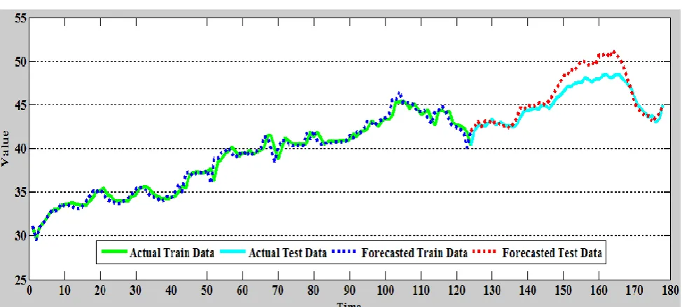
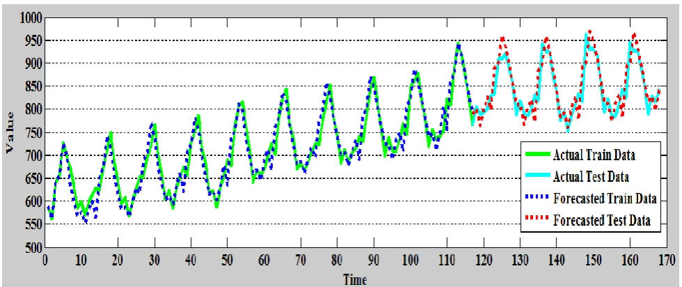
[image:3.595.56.543.475.694.2]From the table 4 and Table 5 it is observed that both the evolutionary neural networks provide better forecast accuracy than ANN-GD method. It is also observed that ANN-DE provides best forecast accuracy among the three methods considered on both the time series. To have a better idea regarding how close the forecasted values to that of true values using ANN-DE, we have plotted comparison shown in Figure 2 and Figure 3.
Fig 3: Forecasted Values using ANN-DE on Milk Production Time Series
5.
CONCLUSION
In this paper, fully connected multilayer perceptron model is considered and three methods like ANN-GD, ANN-GA and ANN-DE are used to predict the future values. It is observed that both the evolutionary methods (ANN-GE and ANN-DE) outperform the gradient based method (ANN-GD) for both the time series considered. It is also observed that the ANN model with differential evolution algorithm performs better than other two models in terms of forecast accuracy. Being an initial effort simple strategies in both preprocessing and learning algorithm are followed. Much more improvements can be done to make the ANN-DE method much more efficient.
6.
REFERENCES
[1] S.G. Makridakis, S.C. Wheelright, R.J. Hyndman, Forecasting: Methods and Applications.
[2] G.P. Zhang, B.E. Patuwo, M.Y. Hu, Forecasting with artificial neural networks: The state of art, International Journal of Forecasting 14 (1988) 35-62.
[3] J. Connors, D. Martin, and L. Atlas, “Recurrent neural networks and robust time series prediction,” IEEE Trans. Neural Netw., vol. 5, no. 2, pp. 240–254, Mar. 1994. [4] C. M. Kuan and T. Liu, “Forecasting exchange rates
using feed forward and recurrent neural networks,” J. Appl. Econ., vol. 10, no. 4, pp. 347–364, 1995.
[5] C. L. Giles, S. Lawrence, and A. C. Tsoi, “Noisy time series prediction using a recurrent neural network and grammatical inference,” Mach. Learn., vol. 44, nos. 1–2, pp. 161–183, 2001.
[6] X. B. Yan, Z. Wang, S. H. Yu, and Y. J. Li, “Time series forecasting with RBF neural network,” in Proc. IEEE Int. Conf. Mach. Learn. Cybern.,vol.8. Guangzhou, China, Aug. 2005, pp. 4680–4683.
[7] F. Liang, “Bayesian neural networks for nonlinear time series forecasting,” Stat. Comput., vol. 15, no. 1, pp. 13– 29, Jan. 2005.
[8] M. Firat, “Comparison of artificial intelligence
[9] Y. Bodyanskiy, I. Pliss, and O. Vynokurova, “Adaptive wavelet-neuro-fuzzy network in the forecasting and emulation tasks,” Int. J. Inf. Theories Appl., vol. 15, no. 1, pp. 47–55, 2008.
[10] W. Yan, “Toward Automatic Time-Series Forecasting Using Neural Networks,” IEEE Transaction on Neural Networks and Learning Systems, vol.23,no.7, July 2012. [11] A. Sorjamaa, Y. Miche, R. Weiss, and A. Lendasse,
“Long-term prediction of time-series using NNE-based projection and OP-ELM,” in Proc. IEEE World Congr. Comput. Intell., Jun. 2008, pp. 2674–2680.
[12] H. Dhari, A.M. Alimi and A. Abraham, “Hierarchical multi-dimensional differential evolution for the design of beta basis function neural network,” Neurocomputing Journal, Elsevier Science, vol.15.pp.131-140, Nov.2012. [13] J. Peralta, G. Gutierrez, A. Sanchis, ADANN: Automatic
Design of Artificial Neural Networks. ARC-FEC 2008 (GECCO 2008). ISBN 978-1-60558-131-6.
[14] J. Peralta, X. Li, G. Gutierrez, A. Sanchis, Time series forecasting by evolving artificial neural networks using genetic algorithms and differential evolution, In Proceedings of the 2010 WCCI conference, IJCNN-WCCI’, (2010) 3999–4006.
[15] J.P. Donate, X. Li, G. G. Sanchez, A.S.D. Miguel, Time series forecasting by evolving artificial neural networks with genetic algorithms, differential evolution and estimation of distribution algorithm, Neural Computing and Application (2011) DOI 10.1007/s00521-011-0741-0.
[16] R. Storn, K.Price, Differential evolution- A simple and efficient heuristic for global optimization over continuous spaces, J. Glob. Optim. 11(4) (1997) 341-359.
[19] K. Socha, M. Doringo, Ant colony optimization for continuous domains, Eur. J. Oper. Res. 185(3) (2008) 1155-1173.
[20] D. T. Pham, A. Ghanbarzadeh, E. Koc, S. Otri, S. Rahim, M. Zaidi, The bees algorithm- A novel tool for complex optimization problems, in IPROMS 2006. Oxford, U.K.: Elsevier (2006).
[21] H.G. Beyer, H.P. Schwefel, Evolutionary Strategies: A Compehensive introduction, Nat. Comput. 1(1) (2002) 3-52.
[22] A. Y. S. Lam and V. O. K. Li, “Chemical-Reaction-inspired metaheuristic for optimization”, IEEE Transactionson on Evolutionary Computation, 14(3), (2010),381–399.
[23] A.Y.S. Lam, “Real-Coded Chemical Reaction Optimization”, IEEE Transaction on Evolutionary Computation, 16(3) (2012), 339-353.