Munich Personal RePEc Archive
The real exchange rate of the rand and
competitiveness of South Africa’s trade
Mtonga, Elvis
University of Cape Town
15 December 2006
Online at
https://mpra.ub.uni-muenchen.de/1192/
T
T
T
h
h
h
e
e
e
r
r
r
e
e
e
a
a
a
l
l
l
e
e
e
x
x
x
c
c
c
h
h
h
a
a
a
n
n
n
g
g
g
e
e
e
r
r
r
a
a
a
t
t
t
e
e
e
o
o
o
f
f
f
t
t
t
h
h
h
e
e
e
r
r
r
a
a
a
n
n
n
d
d
d
a
a
a
n
n
n
d
d
d
c
c
c
o
o
o
m
m
m
p
p
p
e
e
e
t
t
t
i
i
i
t
t
t
i
i
i
v
v
v
e
e
e
n
n
n
e
e
e
s
s
s
s
s
s
o
o
o
f
f
f
S
S
S
o
o
o
u
u
u
t
t
t
h
h
h
A
A
A
f
f
f
r
r
r
i
i
i
c
c
c
a
a
a
’
’
’
s
s
s
t
t
t
r
r
r
a
a
a
d
d
d
e
e
e
Elvis Mtonga1
School of Economics, University of Cape Town
1 5 A u g u s t 2 0 0 6
A b s t r a c t
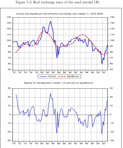
n the last 10 years since South Africa transformed into a democracy, the rand has seen an increase in volatility of its real exchange rate. These fluctuations in the rand’s real exchange rate have raised questions as to whether they signify significant misalignment of the currency and thereby undermine competitiveness of South Africa’s exports abroad. This is a pertinent question in the South African context because foreign trade has been critical to the growth of the economy. Efforts to address current high levels of unemployment and widespread poverty among the majority of the population have depended upon this growth. This study investigates the extent to which fluctuations in the rand’s real exchange rate have impacted on the competitiveness of South African trade flows by determining whether, at some point, the rand had been misaligned, and the likely consequences of such a misalignment. Using data from 1972 to 2003, and an equilibrium correction model of the rand’s real exchange rate drawn on existing literature, the study finds that, from 1994 to 1996, and also in 1998, the rand’s real exchange rate became undervalued by an average 10%. By early 2002, the extent of overshooting had reached 20%. However, the strong recovery of the rand at the start of 2002 reversed this overshooting and instead pushed the real exchange rate above its equilibrium by an average 16 to 17% at the end of 2003. This suggests significant loss of trade competitiveness during 2003 and needed a nominal depreciation to correct the imbalance.
I
1
T
T
a
a
b
b
l
l
e
e
o
o
f
f
c
c
o
o
n
n
t
t
e
e
n
n
t
t
s
s
T a b l e o f c o n t e n t s... i
T a b l e o f c o n t e n t s List of figures ... ii
List of Tables... iii
1 I n t r o d u c t i o n ... 1
2 M e t h o d s f o r a s s e s s i n g r e a l e x c h a n g e r a t e m i s a l i g n m e n t s ... 5
2.1 T he purchasing power parity approach ... 6
2 . 2 T he macroeconomic balance approach ... 8
2.3 T he behavioural equilibrium exchang e rate (BEER) approach ... 10
3 M o d e l l i n g t h e r a n d ’ s e q u i l i b r i u m r e a l e x c h a n g e r a t e a n d a s s e s s i n g t h e e x t e n t o f m i s a l i g n m e n t ... 11
3.1 Factors that determine real exchange rates ... 14
3.2 Empirical Application ... 18
3.2.1 Specification of the empirical model ... 18
3.2.2 Testing methodology ... 19
3.2.3 Data definitions and sources ... 26
3.2.4 Empirical results ... 31
4 C o n c l u s i o n ... 50
List of figures
Figure 1-1: Real Effective Exchange Rate for the rand: 1970 to 2005 2
Figure 3-1: South Africa: fundamental determinants of the real exchange rate 30
Figure 3-2: Real exchange rates of the rand (model 1B) 44
Figure 3-3: Real exchange rates of the rand (model 2A): 1972-2003 45
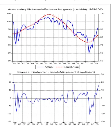
Figure 3-4: Real exchange rates of the rand (model 4A): 1985-2003 46
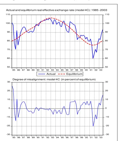
Figure 3-5: Real exchange rates of the rand (model 4C): 1985-2003 47
Figure 3-6: Real exchange rates of the rand (model 5B): 1985-2003 48
List of Tables
Table 3-1: Results of Dickey-Fuller’s unit root tests for stationarity
properties of the data ...32
Table 3-2: Chi-squared statistics for joint VEC lag exclusion Wald
test...36
Table 3-3: Chi-square statistics for joint tests of VEC model
diagnostics...36
Table 3-4: Results of Johansen’s cointegrating test ...37
Table 3-5: Results of estimating co-integrating relationships among
1
I n t r o d u c t i o n
anaging the exchange rate has remained at the centre of South Africa’s efforts to achieving and maintaining both macroeconomic stability and a sustained increase in the growth rate of the economy, ever since the country transformed to democracy in 1994. In this period, the problem of high and rising unemployment, combined with widespread poverty, emerged as the most pressing challenge facing the economy, mainly because of the country’s history of segregation under Apartheid. Economic policy responses to this unemployment challenge have aimed at attaining a sustainable growth rate of the economy, which is seen by the government as a basis for job creation. However, the growth performance of the South African economy has proved insufficient to address the unemployment problem, with the country experiencing a contraction in output for the most part of the early 1990’s, going by the growth in real gross domestic product per capita, which accounts for population growth in measuring the growth rate an economy. Though a rebound in economic growth has occurred since the mid-1990s, this has been too low, peaking just above 2% only in 1996, 2003, and 2004.
M
As the South African economy is highly dependent on the global economy, foreign trade has been critical to growth of the economy2. Stability of the real exchange rate is
thus seen by the Government as key to attainment of its growth objectives, since this not only impacts on global and domestic demand for South Africa’s production but on domestic prices also. Being a relative price of domestically produced goods relative to foreign goods, the real exchange rate provides a measure of how much, on average, the cost of South African produced goods and services will cost relative to a comparable basket of foreign produced goods and services, and therefore of their competitiveness overtime. More so that exports reflect foreign demand of South Africa’s production, their increase means that all output, employment, and incomes associated with their production may increase overtime and thereby contribute to the growth rate of the
2
economy. Unwarranted fluctuations in the real exchange rate, thus, tend to be detrimental to the competitiveness of exports. As such, the Government’s growth and employment objectives may be undermined.
[image:8.612.107.509.374.627.2]However, the rand’s real exchange rate has experienced considerable volatility. As is evident in figure 1-1, which depicts the evolution of the rand’s real effective exchange rate from 1970 through to 2005, fluctuations in the real exchange rate have, at times, been large and persistent for several months. After appreciating strongly in the 1970s by 50 percent from 1972 to1983, the rand collapsed in the early 1980s by 47percent over a space of just two years between 1983 and 1985. Subsequently, the rand rebounded by 44 percent between 1985 and 1994, but weakened again by 41 percent between 1994 and 2001. By December 2003, the level of the real effective exchange rate index represented an appreciation of more than 50% over its December 2001 level.
Figure 1-1: Real Effective Exchange Rate for the rand: 1970 to 2005
60 80 100 120 140 160 180
60 80 100 120 140 160 180
70 72 74 76 78 80 82 84 86 88 90 92 94 96 98 00 02 04 Real effective exchange rate of the rand
(Index: 1995=100)
Source: I-Net Bridge
conventionally, regarded as misaligned when it’s observed values exhibit persistent departures from its long run equilibrium trend, which is the value consistent with long run trends in economic fundamentals (IMF, 1998). In consequence, a misaligned real exchange rate is labelled “overvalued” when its value is higher (appreciates more) than its long run equilibrium value, and “undervalued” once it falls (depreciates) below the equilibrium value. Thus, to make an assessment of real exchange rate misalignment, a measure of the equilibrium real exchange rate is often required as this forms a benchmark against which the actual or observed real exchange rate can be gauged (Maeso-Fernandez, et al, 2001).
This question of whether or otherwise the rand’s real exchange has, at any point in time, been misaligned is pertinent to South Africa given, as already noted, the importance to the economy of foreign trade and capital flows. In such an environment of greater openness of the economy, misaligned real exchange rates are known to have the potential to impose large costs to the economy, in the sense of having an adverse effect on resource allocation in the economy. When a country’s real exchange is overvalued, the implication is that domestic goods become more expensive relative to foreign goods, since it reflects the price of domestic goods relative to foreign goods. This has the potential of increasing the demand for foreign goods at the expense of domestically produced goods, and as a result, there will be considerable scope for imports to increase, while the production of domestically produced import substitutes is more likely to decline. Because of the increase in the cost of producing them, and the associated loss of profitability, exports will be harmed. Thus, overtime, a country’s external position will tend to deteriorate, and rising unemployment may accompany this.
overtime, there will be tendency for country’s balance of payments to improve, as well as the employment situation.
The adverse effects of real exchange rate misalignment are, thus, well recognized in the literature. However, the significance of these often different and complex effects of changes in the real exchange rate will, in many instances, depend of the economic conditions prevailing in the country, such as whether the economy is in recession or boom (De Kock Commission of Enquiry, 1985). Much also depends on the prevailing stance of other policies, such as fiscal and monetary policies, which may strengthen or weaken the transmission of these exchange rate effects to rest of the economy. While this may seem to suggest that the adverse impacts of real exchange rate misalignment are not automatic, an understanding of the extent of real misalignment is nonetheless important, as if such misalignments were to be large, this may serve to suggest the likely costs that the economy is likely to face in the future, if no adjustments to domestic policies are made.
Thus, we investigate, in this study, the extent to which past movements of the real exchange rate of the rand have impacted on the competitiveness of the South African trade flows by determining whether at some point the rand had been “misaligned” or otherwise, and the likely consequences of such a misalignment. Because “misalignment” is with reference to some benchmark equilibrium measure, we identify the variables that are fundamental in valuing the rand, which we then use to estimate a long run model of the rand’s real exchange rate. Based on the findings of the long run real exchange rate model, we derive a long run equilibrium real exchange rate value for the rand, which we compare with the observed real exchange rate so as to make judgment on whether or not the rand has been “misaligned”.
restrictions to have been the main determinants. However, the study did not probe the issue misalignment in the real exchange rate. Using data from 1970 to 2002 and a somewhat smaller set of explanatory variables, MacDonald and Ricci (2003) also estimated an equilibrium real exchange rate model for the rand, which they used to measure the degree of misalignment. Their analysis showed that, in early 2002, the rand had overshot its equilibrium value by at least 25%. Similarly, Samson et al (2003a, b) found that the rand’s real exchange rate had become significantly undervalued in 2002, following a prolonged period of considerable depreciations during 2001. Previous studies are thus confirmatory of the important of economic fundamentals in providing useful information to understanding movements in the rand’s real exchange rates.
Our study adds to this literature in two ways. Firstly, we test for the significance of additional variables and employ a somewhat different specification. Secondly, we use a large sample and test our model across two different sample periods.
In terms of organisation, the rest of the discussion has been structured as follows. Section 2 examines the literature on the analytical and methodological framework connected with estimation of equilibrium real exchange rates and assessment of real exchange rate misalignment. Next, in section 3, we discuss the empirical approach adopted by the study, beginning first with a discussion of the theoretical model, and then the econometric methodology used to analyze the relationship between the real exchange rate and a set of economic fundamentals considered and the empirical results. Finally, we conclude the discussion, in section 4, with a presentation of a summary of main findings.
2
M e t h o d s f o r a s s e s s i n g r e a l e xc h a n g e r a t e
m i s a l i g n m e n t s
v
unobservable and have to be calculated based on an analytical framework3. This poses
the difficult that, in the literature, one finds multiple analytical frameworks, which give rise to different empirical values for the real exchange rate to choose from.
On one hand, economists have focused on the so called external real exchange rate, which is derived as a ratio of the home to the foreign value of a broad based price index, where both prices are denoted in the same currency (Hinkle & Montiel, 1999). However, matters are complicated by the fact that there exist multiple price indices to choose from, with the implication that there are as many empirical real exchange rates as there are price indices (Mark, 2001). On the other hand, the real exchange rate has been defined as a relative price of tradable goods in terms of non-tradable goods, and this is labelled the internal real exchange rate (Hinkle & Montiel, 1999). Even with this approach, multiplicity of conceptual definitions give rise to several estimates of the real exchange rate, thus raising the question as to when it might be appropriate to use one rather than the other. Nonetheless, subject to these conceptual and empirical ambiguities, three alternative methods have been widely used to assess misalignments in real exchange rates.
2.1 T he purchasing power parity approach
The purchasing power parity (PPP) approach is the basic methodological framework often used for the empirical examination of real exchange misalignments. This approach is based on the law of one price, which holds that if markets are competitive and there is free trade of goods between them, the same basket of goods and services should command the same price across all markets when expressed in a common currency. To the extent that the law of one price held true, the implication is that the nominal exchange rate that ensures convergence of prices of a common basket of goods and services between two countries constitutes an equilibrium value for the nominal exchange rate, which is labelled the PPP-exchange rate (Clark, et al, 1994).
3
If for some reason the market exchange rate significantly differed from the PPP-exchange rate, then profits can be made by buying the common basket of goods in the low price market and selling it in the high price market, a situation that will eventually tend to push the exchange rate back to its PPP equilibrium value overtime. In consequence, PPP predicts that the real exchange rate remains unchanged overtime, starting from a position of equilibrium in a base year when a country’s balance of payments position was judged to be sustainable (International Monetary Fund, 1998). Assessing real exchange rate misalignment under the purchasing power parity approach then involves a comparison of prices of a basket of goods produced by the home country with that of a comparable basket abroad and calculating the exchange rate that would equalize them, relative to a base year in which the balance of payments was judged to be sustainable (Wren-Lewis, 2003). If its current rate is higher or lower relative to its level in that base year, then the real exchange rate is misaligned.
2 . 2 T he macroeconomic balance approach
The empirical criticisms of the purchasing power parity approach discussed above have led Williamson (1985, 1994a, b) and Isard and Faruqee (1998) to advocate the macroeconomic balance approach to assessing misalignments in real exchange rates4. This entails calculating the equilibrium real exchange rate as the rate that simultaneously yields the economy’s internal and external equilibrium. External equilibrium is taken to mean achievement of a sustainable current account deficit, meaning one that can be financed without undue foreign borrowing or an unnecessary loss of foreign reserves (International Monetary Fund, 1998). Internal balance, on the other hand, is defined as the level of output corresponding to full employment and low inflation or macroeconomic stability. As the equilibrium real exchange rate depends on internal and external balance, it will change once this position changes. The equilibrium exchange rate is, therefore, thought of as a range of equilibrium exchange rates rather than a single number and changes overtime consistent with fluctuation of its fundamental determinants (International Monetary Fund Institute, 1998).
In addition, the approach incorporates explicitly the time horizon in its notion of equilibrium. This implies that the real exchange rate should be considered to be in equilibrium only in the context of economic fundamentals determining internal and external equilibrium over a given time frame (Hinkle & Montiel, 1999). This follows because economic fundamentals that may be relevant for achievement of internal and external equilibrium at say a short run period may differ from those ones with the most influence over a much longer time horizon. Thus, in practical applications, researchers often select a different set of economic fundamentals defining both internal and external equilibrium, and therefore a different value for the exchange rate, depending on the time horizon under investigation (Clark et al, 1994). In this respect, the macroeconomic balance represents a major advance over the purchasing power parity approach.
4
However, it has its drawbacks also. One is that the approach is a method for calculating equilibrium real exchange rates, rather than a theory of exchange rate determination and does not therefore embody theoretically testable predictions. The other relates to the fact that though the macroeconomic balance provides a precise description of internal and external equilibrium, and therefore of the equilibrium real exchange rate, this is difficult to determine in practice. When exactly an economy’s macroeconomic equilibrium prevails in practice can not be easily discerned. For this, one would require a macroeconomic model that accurately captures relationships defining current account balance, full employment level of output, and inflation. But, the practicality of constructing such a model is often hampered by resource constraints.
Thus, in empirical applications, researchers have attempted to overcome the latter problem by employing theoretical models designed to seek a set of economic relationships describing an economy’s output and balance of payments position, and where the value of underlying determinants have been set at their full employment or sustained levels (Clark & MacDonald, 1998). The real exchange rate calculated from such an exercise is labelled the “fundamental equilibrium exchange rate” (FEER), reflecting the emphasis on fact that only those factors judged to be important over the medium to long term period should be considered in its derivation, abstracting from transitory factors.
Applying this approach, some researchers have used large econometric models5, for
example, Williamson (1994b), who used several macroeconomic models to estimate equilibrium real exchange rates for currencies of the major industrial countries in the 1990s. His analysis revealed significant deviations of real exchange rates from their implied equilibrium values. So too did Bayoumi et al (1994), Faruqee et al (1996), Wren-Lewis and Driver (1997), Wren-Wren-Lewis (2003), and Rosenberg (2003). Other researchers have applied relatively small theoretical models, using empirical estimates of underlying parameters to establish the relationship among output, the balance of payments position,
5
and the real exchange rate. An example is Stein (1995) who calculated equilibrium real exchange rates by estimating regression models of the real exchange rate with several macroeconomic variables. Infact, most studies employing the macroeconomic balance approach have focused on industrial countries.
2.3 T he behavioural equilibrium exchang e rate (BEER) approach
Finally, a more recent method is the behavioural equilibrium exchange rate (BEER) approach. Pioneered in Clark and McDonald (1998, 2000), the BEER approach is a modelling strategy designed to seek a long run relationship between observed real exchanges and a set of fundamental determinants derived from a theoretical real exchange rate model. Its has the attractive feature that the real exchange rate is required to be in equilibrium only in terms its value given by the appropriate set of explanatory variables over a specific sample period. This allows representation of the equilibrium real exchange rate in terms of the dynamic structure that generates the data on the real exchange rate and its fundamental determinants (Hinkle & Montiel, 1999), even though the variables themselves are derived from a long run structural model.
Application of the BEER approach requires, as a first step, specification of a behavioural relationship of the real exchange rate and a set of economic fundamentals drawn from a reduced-form theoretical model. This relationship is then estimated to establish the long run impact of fundamental determinants on the real exchange rate. However, since current values of fundamentals may include the influence of transitory factors, the approach also requires judging whether the economic fundamentals determinants themselves are at their long run or sustainable values (Clark & McDonald, 1998). On this, a common practice in the literature is to calibrate values of explanatory variables using a detrending filter such as Hodrick and Prescott’s (1997) H-P filter or Beveridge and Nelson (1981) decomposition, both of which decompose a time series variable into its long run trend and short run cyclical value.
real exchange relationship to establish the long run equilibrium real exchange rate. Finally, an assessment of misalignment is made by comparing the value for the real exchange generated by this relationship containing de-trended values for the economic fundamentals with the actual value for the real exchange rate. However, because of differences in methodological approaches to identifying fundamental determinants, and those of estimating these relationships, the BEER approach tends to yield different values for the equilibrium real exchange rates and the extent of their misalignments.
All the same, there is somewhat extensive application of the BEER approach to analysis of currencies of developing and middle-income economies. An influential study is Edwards (1989) who applied the methodology to 12 developing and middle income countries from 1962 through to 1984, and found significant misalignments in their currencies. So too did Elbadawi’s (1994) study of currencies for Chile, Ghana, and India, and Baffes et al (1999) for Cote d’Ivoire. More recently, Manthisen (2003) used a theoretical model drawn on Edwards (1989) to investigate real exchange rate misalignment in Malawi and found several episodes during which the Malawan Kwacha had experienced several misalignments. However, Cady (2003) found that the Malagasy franc did not seem to have experienced any major misalignments for the most of the 1990s. There is therefore confirmation in the literature that real exchange rates are predictable based on their underlying determinates, despite variations in methodologies used to estimate them.
3
M o d e l l i n g t h e r a n d ’s e q u i l i b r i u m r e a l e xc h a n g e r a t e
a n d a s s e s s i n g t h e e x t e n t o f m i s a l i g n m e n t
In Montiel’s model6, the real exchange rate is defined as the relative price of
non-traded goods in terms of non-traded goods, and the long run equilibrium exchange rate is that rate that is consistent with achievement of internal and external equilibrium, when underlying determinants are at their sustainable values. The model develops on the basis of a small open economy with a fixed exchange rate system, financially open to international financial markets, and flexible domestic wages and prices. The production side of the economy consists of producers who produce traded and non-traded goods, and are price takers in the world market. Output in each sector is produced with a fixed, sector-specific, homogenous, and freely mobile labour input, which is also subject to diminishing marginal returns. In both sectors, producers make their allocation decisions on the basis of profit maximization object by setting the marginal product of labour to the wage rate.
The demand side of the economy is modelled in terms of the behaviour of households and the public sector. The behaviour of the representative household reflects its actions to maximize current and future discounted consumption of both the traded and the non-traded good, subject to a wealth constraint, which also determines the path of consumption expenditure. At each period, the actions of the representative household are such that it decides to allocate its net worth between net foreign bonds (financial assets) and domestic money. Bonds can be held either in domestic currency, which pays a nominal interest rate , or foreign currency, which pays a nominal interest rate, , and the two interest rates are related through an arbitrage relationship described by the uncovered interest rate parity condition. The holding of domestic money, on the other hand, is motivated by the desire to reduce transaction costs related to consumption. This allocation decision defines the representative household’s wealth constraint.
r r∗
The public sector, on the other hand, is a consolidated public sector, made up of the government and the central bank. The central bank’s functions are to manage the exchange rate, which it achieves by exchanging domestic currency for foreign currency
6
upon demand, and providing credit to government. In addition to receiving credit form the central bank, the government also receives lump-sum taxes from the private sector, which it uses to consume traded and non-traded goods.
With regard to the external position, the country can borrow from and lend to the rest of the world, since the economy is financially open to the rest of the world. However, its financial liabilities are deemed imperfect substitutes for those of the rest of the world. Given this, the rate at which its residents can borrow from or lend to the rest of the world reflects a risk premium, which reflects the country’s ability to borrow or its international indebtedness. This is defined by the uncovered interest rate parity arbitrage condition, adjusted for a risk premium.
Given the actions of households, the government, and the country’s relationship with the rest of the world, the model, when solved, implies an external and external equilibrium condition for the economy. External equilibrium is attained when the level of consumption and the real exchange yield a sustainable current account balance. This equilibrium condition is represented by the following relationship:
T
T e r a c g
y
a∗ = + ∗ ∗ − ∗ + −
∗
) (
)
( τ θ
π (1)
Where is the world inflation rate, is the net foreign assets of the country, is traded goods output, inversely related with the real exchange rate,
∗
π ∗
a yT(e)
e is the real exchange rate [measured as the relative price of non-traded goods in terms of traded goods], is the foreign nominal interest rate, is interest receipts on net foreign assets, is the transaction costs associated with consumption,
∗
r
∗ ∗
a
r τ∗
θis the share of traded goods in total consumption, and gTis government consumption of traded goods.
assets adjusted for inflation. These two components together underscore the idea that, in the long run, the real current account must equal the real value of a country’s claims on the rest of the world. Because traded goods’ output is inversely dependant on the real exchange rate, a fall of its consumption appreciates the real exchange rate.
With regard to internal equilibrium, this holds when the market for labour and the non-traded good clears. This is defined by the following relationship:
(
)
NN N
N e c g ce g
y ( )= + = 1−θ + (2)
Where denotes total production of non-traded goods, which is positively related to the real exchange rate, is total private consumption of the non-traded good, measured in terms of the traded good, is government consumption of the non-traded good. Given the positive relationship between non-traded goods’ production and the real exchange rate, increased household and government consumption of the non-traded good will increase its production, and hence appreciate the real exchange rate.
N
y
c
N
g
3.1 Factor s that deter mine real exchange rates
Since the equilibrium exchange rate is given as that rate which is consistent with simultaneous achievement of external and internal equilibrium, factors determining this macroeconomic balance condition constitute the real exchange rate’s fundamental determinants. In the framework of Montiel’s model7, these are identified as domestic
supply side factors, the stance of fiscal policy, changes in the international financial environment, and the stance of trade and commercial policy.
Domestic supply-side factors
A candidate variable for changes in domestic supply related factors is the relative productivity growth rate between a country and its trading partners, first suggested by Balassa (1964) and Samuelson (1964) and is often referred to as the Balassa-Samuelson
7
effect. Balassa and Samuelson’s argument is that if a country were to experience a productivity shock that increases production in its tradable goods sector relative to its non-tradable goods sector, this would have the effect of appreciating the equilibrium real exchange rate. This would follow because increased output of tradable goods would permit an increase in demand for labour in favour of this sector, and hence the real wage. Resulting from this, a shift in labour from the non-tradable goods sector would be expected, which, at the given real exchange rate, would mean an expansion of the tradable sector while the tradable sector would contract. This would have the effect of creating excess demand in the non-tradable goods sector; thereby give rise to a higher relative price tradable. By increasing production of tradables relative to non-tradables, the productivity shock also gives rise to a trade surplus, which means that the real exchange rate would have to appreciate to maintain eternal equilibrium. Accordingly, countries that experience higher rates of productivity growth in their tradable goods sectors relative to their trading partners are expected to experience appreciations of their real exchange rates (Aghevli et al, 1991).
Stance of fiscal policy
Fiscal policy has an ambiguous effect on the equilibrium real exchange rate: the direction of its quantitative influence depends on the sectoral composition of the change in government expenditure. If government increased its expenditure on tradable goods, this would have the effect of increasing demand for tradable goods through an increase in import consumption, thereby creating a trade deficit. To maintain external equilibrium, a depreciation of the real exchange rate would be required. By contrast, increased government expenditure on non-tradable goods will tend to create excess demand in the non-tradable goods market. To maintain goods market equilibrium, an increase in the relative price of non-traded goods would be required, thereby appreciating the real exchange rate. Thus, changes in the stance of fiscal policy can either depreciate or appreciate the real exchange rate.
Aspects of changes in a country’s international economic environment considered in the literature include changes in the terms of trade. Here an improvement in a country’s terms of trade, which refers to an increase in the price of its exportable goods relative to importable goods, is expected to appreciate the real exchange rate. This follows because increases in the price of exports permit an expansion of the export sector output, and thus gives rise to excess supply of exportable goods and a trade surplus. This increase in export sector output would allow an increase in the real wage in the traded goods sector relative to that of the non-traded goods sector. As a result of this, a redistribution of labor from the non-traded to the traded goods sector would be expected. At the same time, output of non-traded goods would be expected to contract, thereby creating excess demand in the non-traded goods market, and thus a higher relative price. Both the improvement of the trade balance and the rise in the price on non-tradable goods require an appreciation of the real exchange rate if equilibrium is to be maintained. However, MacDonald and Ricci (2003) point out that “in practice few studies find the terms of trade variable to be significant” largely on account of the arbitrariness involved in calculating this variable (p. 4). Thus an alternative approach used has been to proxy the terms of trade variable with real commodity price movements of major commodity exports, which is not only an accurate measure particularly for major commodity exporters, but has also received empirical support (MacDonald & Ricci, 2003).
Another factor connected to the change in a country’s international financial environment is the flow of international capital and transfers. Increases in the flow of capital imply a higher net foreign asset position of the country, which increases the country’s level of real income. This then permits a larger expenditure on domestic (non-tradable) goods (MacDonald & Ricci, 2003), creating excess demand and a rise in the price of non-tradable goods. As a result, an appreciation of the real exchange rate would be expected.
to that of its trading partners, representing say aggregate demand conditions, productivity levels, or persistent tightening of monetary policy (MacDonald & Ricci, 2003), creates opportunities for capital to flow to that country. As a result, an improvement of the current account would be expected, thereby appreciating the real exchange rate.
By contrast, changes in the world inflation rate will tend to cause a depreciation of the equilibrium real exchange rate. The transmission mechanism for this is through the effects of inflation on transaction costs associated with changes in the real demand for money. The direction of such transactions costs on the equilibrium real exchange rate will tend to depend on whether they are incurred through consumption of traded or non-traded goods, which in both cases, reduces their supply. In the case of traded goods, this would require a real exchange rate appreciation. For non-traded goods, the implication is that the real exchange rate should depreciate. To the extent domestic prices reflect the relative price of non-traded goods, a higher domestic inflation for a country relative to that of its trading partners would imply a depreciation of its real exchange rate.
Stance of trade and commercial policy
3.2 Empirical Application
3.2.1 Specification of the empirical model
On the basis of theoretical motivations discussed above, we expect the following factors to influence real exchange rate movements of the rand,
• the real interest rate differential vis-à-vis South Africa’s main trading partners,
• the inflation differential vis-à-vis South Africa’s main trading partners,
• variations in the terms of trade for South Africa,
• the level and composition of government expenditure [stance of fiscal policy],
• relative technological or productivity progress [proxy for Balassa-Samuelson effect] vis-à-vis South Africa’s main trading partners,
• international capital flows,
• openness of the trade regime [proxy for the stance of commercial and trade policy],
• the stock of foreign currency reserves, and
• the stock of foreign debt.
Accordingly, our empirical model has the following specification:
t t
t F
q =α +β′ +ε (3)
Where denotes the rand’s real exchange rate, and is a vector of fundamental variables mentioned above,
t
q Ft
βis a vector of coefficients, and εtis a random error term.
Specifically, where is
the real interest rate differential for South Africa relative to its main trading partners, is the inflation differential, is the terms of trade, is government
] , , , , , , ), ( ), [( − − ′ = ∗ ∗ t t t t t t t t t t t
t r r tot gxp prod ka open fx fxb
F π π rt −rt∗
∗
− t t π
consumption (expenditure), is relative productivity growth (proxy for
Balassa-Samuelson effect), is international capital flows, a measure for openness of
the trade regime, is foreign currency reserves, is foreign debt, and the asterisk denotes foreign variables.
t
prod
t
ka opent
t
fx fxbt
) (∗
The real interest rate differential, terms of trade, productivity growth, capital flows, and foreign reserves all enter the model with a positive sign, since these variables are expected to appreciate the real exchange rate. Conversely, the inflation rate differential, trade openness, and foreign debt variables depreciate the real exchange rate, and are thus specified with a negative sign, whereas as the expected impact of government expenditure is ambiguous.
3.2.2 Testing methodolog y
In the specification discussed above, the object of interest is one of testing whether a long run relationship exists between the rand’s real exchange rate with this set of fundamental determinants by estimatingβ , the vector of parameters. Our choice of the methodology to accomplish this was dictated by properties of our data. Together with other macroeconomic variables, exchange rates appear to possess non stationary stochastic trends that allow variables to grow overtime with no tendency to revert to their mean values. The presence in the data of such non stationary stochastic trends is known to invalidate standard statistical inferences. Thus, we employed cointegration analysis, which addresses this non stationary problem in the data. Cointegration tests have the benefit of allowing one to test for and estimate equilibrium relationships among variables and the adjustment process to such equilibrium, even though the processes that generate the data are themselves non stationary stochastic trends.
as a vector autoregressive (VAR) process, and “models the relationships among the variables using a vector equilibrium correction specification” (Cady, 2003, p.4). This starts with examining a VAR model of the following form:
t t p i i t i
t a a t Z B w U
Z = + +
∑
Ψ + +=1 − 0
1
0 (4)
Where Ztis an nx1 vector of jointly determined non-stationary I
( )
1 variables (here is the number of variables in Z), is a vector of exogenous stationary[ ]variables, tis adeterministic trend variable,
n
t
w I(0)
0
α is a vector of intercept coefficients, Ψi is an matrix of
coefficients, is vector of coefficients on exogenous stationary variables, and is an vector of white noise error terms.
nxn
o
Β nx1 Ut
1
nx
When cointegrating relationships are present among the jointly determined variables, the above vector autoregressive process gives rise to a dynamic vector equilibrium-correction [error-equilibrium-correction] model (VECM), which is essentially “a restricted vector autoregressive process that has co integration restrictions built into the specification” (Eviews3.0 Users Guide, p.504). This specification follows from Engle and Granger’s (1987) representation theorem which says that if a group of non-stationary data processes are co integrated, they can be regarded as having been generated by an equilibrium correction process that restricts the long run behavior of jointly determined variables to their long run values while allowing for a series of partial adjustments over the short run (Maddala & Kim, 1998). Hence we may rewrite the VAR process into its VECM form as follows;
t t p i i t i t
t a a t Z Z B w U
Z = + +Π + ΓΔ + +
Δ
∑
−= − − 0 1 1 1 1
0 (5)
Where
∑
nd .= Ψ − Ι − = Π p j j 1 )
( a
∑
− = Ψ − Ι − = Γ 1 1 ) ( p i i i
Here denotes a matrix of long run coefficients that defines long run relationships among the variables, while is a coefficient matrix capturing short run dynamic adjustments among the variables (Pesaran & Pesaran, 1997).
Π
i
When specified in this VECM form, a vector autoregressive process has the advantage of providing information on both the long run relationships among the variables and their short run adjustment to such long run equilibrium relationships. To begin with, since the matrix contains the long run coefficients that underlie long run relationships among the variables, the relation
Π
t
Z
Π represents the long run equilibrium
relationships among the variables. The relations contained in the lagged term serve
as equilibrium correction devices that ensure that the short run adjustments of variables are tied to their long run values overtime. Secondly, the terms
1
−
ΠZt
i t
Z−
Δ represent the short
run dynamics or deviations of the variables from their long run equilibrium, whose impact is represented by . Since cointegration is assumed in this formulation, is
stationary, as is considering that is itself a non-stationary process. As a result, the vector error-correction model is a stationary process, which allows application of standard inference statistics even though the elements of the system are themselves stationary. The vector error-correction model is thus appropriate to model non-stationary data processes that are cointegrated.
i
Γ ΠZt−1
i t
Z−
Δ Zt−i I(1)
Because the matrix contains long run coefficients, and thus provides information on about long run relationships among the variables, the presence of co integration among the variables is indicated by the rank of this matrix, which requires finding
Π
r, the number of linearly independent columns that are present in the matrix. Three cases are distinguishable in this respect:
Case (I). If the matrix Π is of full rank, corresponding to r =n(where equals the number of variables in the system), then there exist
n
n
r= linearly independent columns in the matrixΠ . In this case, the variables in are stationary, and no co-integration exists among the variables. A VAR model with variables specified in their levels is thus the appropriate model.
t
Z
Case (II). On the other hand, if the rank of the matrix Π is zero, when the elements in are non-stationary, then no cointegration exists among the variables. A VAR
t
model with variables specified in their first differences in the appropriate model in this case.
Case (III). Finally, if the matrix Π of reduced rank when the elements in are non-stationary, then there exist at most
t
Z
1 − ≤n
r linearly independent columns in the matrix , which indicates the presence of co-integrating relations in . In this case, the VECM specification is the appropriate framework for modelling the relationships among the variables.
Π r
t
Z
Accordingly, the hypothesis of the existence of co integrating relationships among the variables can be formulated in terms of a hypothesis of the reduced rank of matrixΠ . This can be stated as follows:
1
0 r rank =r≤n−
H ( ): (Π) .
Under this hypothesis of co integration (i.e. case iii above), the pie matrix is equivalent toΠ =αβ′, which flows from Engle and Granger’s (1987) representation theorem. Here α is a full column rank n×r matrix representing the speed of adjustment of variables in
the model, whereas the matrix β is also a full column rank n×r matrix of long run coefficients, with the property that β′Ζt is stationary. In the light of this decomposition of the pie matrix, the vector error-correction model can be written as follows:
t t p i i t i t
t a at Z Z B w U
Z = + + ′ +
∑
+ +− = − − 0 1 1 1 1
0 αβ ΓΔ
Δ (6)
In this vector error correction specification of the VAR model, the stationary cointegrated relationships among the variables are now defined byξt =β′Ζt−1, and this characterizes
the long run relationships among the variables. As a result, the hypothesis on the rank of the matrix is now equivalent to formulating a hypothesis about the rank of the matrix
Π
β′, which has the implication that each column of β′is the cointegrating vector
1 ) ( ) ( : ) (
0 r rank Π =rank ′ =r ≤n−
H β
Testing for cointegration therefore requires an estimate of the pie matrixΠ =αβ′.
In the Johansen’s approach, this is achieved by estimating the pie matrix β
α
Π = ′from the unrestricted VAR model, and then testing whether the restrictions
imposed by the reduced rank of matrix Π can be rejected by the data (Eviews5.0 Users Guide, p. 724). This is tested using two types of tests advocated by Johansen. The first is the trace statistic, which allows one to perform a log likelihood ratio (LR) test for the null hypothesis that there exist r co integrating vectors against the alternative of co integrating vectors (where is the number of endogenous variables in the VAR). This statistic is computed as follows:
n n
∑
+ = − − = − − = − = n r i itrace Q T r n n
LR 1 ) 1 , 2 , , 1 , 0 ( ) ˆ 1 log( ) log(
2 λ K
The second is the maximum eigenvalue (λ−max ) statistic. This is a log likelihood test that tests the null hypothesis that there is r co integrating vectors against the alternative that there is r +1 co integrating vectors. This statistic is computed as follows:
) 1 , 2 , , 1 , 0 ( ) ˆ 1 log( 1
max =−T − + r = n− n−
LR λr K
Asymptotic critical values for conducting these two tests have been provided by Johansen (1988), and also Osterwald-Lenum (1992).
investigation (Eviews5.0 User’s Guide, p. 724). Because of this, the underlying data trends would have to be ascertained prior to implementing the tests. On this, five trend assumptions on whether the data series contain intercepts and or time trends, and whether the intercepts and or time trends are restricted (i.e. form part of the co integrating relations) are distinguishable (Pesaran & Pesaran, 1997)8:
Case (I). The level series data have no trends and the co integrating relations have no intercepts (i.e.a1 =a2 =0).
Case (II). The level of the data have no deterministic trends and the co integrating relations have intercepts (i.e. restricted intercepts and no trends in co integrating relations, a1=0 and a0 =Πρ0where ρ0 denotes an intercept
coefficient).
Case (III). The level data have linear trends but the co integrating relations have only intercepts (i.e. unrestricted intercept and no trends,a1=0 and a0 ≠0).
Case (IV). Both the level data and the co integrating relations have linear trends (i.e. unrestricted intercept and restricted trend, a0 ≠0and a1=Πγ0where
0
γ denotes a trend coefficient).
Case (V). The level data have quadratic trends and the co integrating relations have linear trends (i.e. unrestricted intercept and trend, a0 ≠0anda1≠0).
In practical application, determination of the number of co integrating relations using the Johansen’s method is a sequential process conditional on the trend case assumption discussed above, testing first the hypothesis thatr =0, and then proceeding to r =n−1 until the test fails to reject the hypothesis. After determining the number co integrating relationships among the variables, the next step is to estimate of the vector equilibrium-correction model in order to examine the long run predictability and short run forecasting ability of the model.
8
Tests for the order of integration of variables
However, testing for cointegration is valid only when the variables are generated by a non-stationary process. Ascertaining the order of integration of the data under investigation is therefore a key preliminary step to its application. One widely used methodology for testing the order of integration of variables, which this study employs, is Dickey and Fuller’s (1979, 1981) DF and ADF tests. This tests whetherρ=1, which is a test for existence of a unit root, assuming that the time series data under investigation is generated by a first order autoregressive process of the following form:
t t
t t s
s =α0+α1 +ρ −1+ε (7)
Where α0 is a constant, tis a deterministic trend, andεt, is a white noise stochastic process. Alternatively, the above autoregressive process can be written as follows.
t t
t t s
s =α +α +γ +ε
Δ 0 1 −1 (8)
Whereγ =ρ−1.
t p
i
i t i t
t t s s
s =α +α +γ + βΔ +ε
Δ
∑
−= +
−
1
1 1 1
0 (9)
Under the null hypothesis of a unit root process, the distribution for the t-statistic is not asymptotically normal, and as such, one cannot use the usual t-test to assess the statistical significance ofγ . Nevertheless, Dickey and Fuller have provided appropriate critical values for testing the unit root hypothesis. But, these have since been revised and extended by MacKinnon (1991), who has provided estimates that are appropriate for any sample size (Eviews 3.0 Users Guide, p. 329).
3.2.3 Data definitions and sources
We employed a data set on variables consisting of quarterly observations from the first quarter of 1970 to the fourth quarter of 2003, which we obtained from I-Net Station Bridge online statistical database, International Monetary Fund’s International Financial Statistics (IFS) online database, and South African Reserve Bank’s (SARB) online database. A more detailed description of the variables and their data sources is given below, while their graphical presentation during the period under review is given by figure 3-1.
Real exchange rate
We used the CPI-based real effective exchange rate index (REER) for the rand, calculated by the South African Reserve bank as the average value of nominal bilateral exchange rates of the rand with respect to 13 countries, weighted by the volume of trade between South Africa and these countries and adjusted for movements in their respective consumer price index differential9. Its definition here in terms of foreign
currency per unit of the rand, so that an increase in the real effective exchange rate denotes an appreciation. The weighting structure used in the calculation of the index is described in South African Reserve Bank (1999), and this is based on the methodology described in Zanello and Desruelle (1997). Of the thirteen currencies in the basket, the
9
four major currencies are the euro, with a weight of 36.30%, the British pound with 15.37%, the US dollar with 15.47%, and the Japanese yen with 10.43%. Together, these four major currencies account for 77.6% of total weighting of the basket. This variable is expressed in logarithms as LREER and the data was obtained from I-Net Station Bridge.
Real Interest rate differential
This is the real yield rate on the 10 year South African government bond relative to the real yield rate on the 10-year government bond for trading partner countries. The real interest rate was calculated as the nominal interest rate minus four-quarter CPI-inflation rate for each country. For the trading partner countries, this was calculated as a weighted average of four major trading partners based on trade weights for the real effective exchange10.The weights used for the four major trading partner countries [shown in brackets] are the following: Germany (proxy for the European Union, 42%), United States (21%), United Kingdom (21%) and Japan (16%). This variable is denoted
RGBRDD. The data source for nominal interest rate on the 10 year government bond and consumer price index for each country is the IFS.
Fiscal position
We employed two alternative measures for the fiscal position variable. One which we have denoted FBA is the ratio of the fiscal balance (budget deficit) to Gross national Product (GDP) expressed as percentage. The data source for this variable is South African Reserve bank (SARB). The other which we have denoted GVERT is the ratio of government expenditure to GDP expressed as a percentage. The source of data for this measure is I-Net Station Bridge.
Terms of trade
We used three alternative measures for the terms trade variable, all expressed in natural logarithms. The measure denoted LGOLPRN is an index of the real gold price normalized to 1 in 2000, defined as the London market US dollar price of gold deflated by the US consumer price index11. The data source for this series is IFS. The other
10
See also MacDonald and Ricci (2003)
11
measure which we have denoted LTOTGN is an index of the ratio of exports prices to import prices including the price of gold, normalized to 1 in 2000. Finally LTOTN is an index of the ratio of export to import prices excluding the price of gold, also normalized to 1 in 2000. The data source for both the latter series is SARB.
Productivity growth differential
No source data is available for this variable. However, in the empirical literature, this variable is often proxied by other closely related variables on which data is available such as real GDP per capita or variables connected to measures of education and demographic factors (Egert, 2002, p.5). In line with this approach in the empirical literature, we measured this variable by relative real GDP per capita, which effectively measures labour productivity as real GDP divided by total population, and is meant to capture the effects of labor productivity increases of the home country relative to the foreign country (Maeso-Fernandez, 2001, p. 13). The foreign variable used in the calculation was measured as a weighted average of real GDP per capita for the four trading partner countries, based on weights for the real effective exchange rate, and normalized to 1 in 2000 for each country. This variable is expressed in natural logarithms and is denoted LGDPRKDN. The data source is SARB for South Africa, and IFS for the four trading partner countries.
Trade and commercial Policy
This was measured by an openness variable, calculated as the ratio of the sum of exports and imports (i.e. total trade) to GDP, and expressed as a percentage. This variable is denoted OPEN, and the data source for the export, the import, and the GDP variable is SARB.
Foreign reserves
We employed two measures for the stock of foreign reserves. The first, denoted as
Inflation differential
This is the four-quarter CPI inflation rate for South Africa minus the four-quarter CPI for the four trading partner countries, with the foreign variable computed in similar manner as above. This variable is INFLRD, and the source for the data is IFS.
Foreign debt
This is the ratio of total foreign debt for South Africa to GDP, in percentage. This variable is labelled FXTBR, and the data source is INet Station Bridge.
Capital flows
We employed two measures for the capital flows variable. The series labelled NTFDI
Figure 3-1: South Africa: fundamental determinants of the real exchange rate -10 -5 0 5 10
1970 1975 1980 1985 1990 1995 2000 RGBRDD -16 -12 -8 -4 0 4 8
1970 1975 1980 1985 1990 1995 2000 FBA 3 4 5 6 7 8 9
1970 1975 1980 1985 1990 1995 2000 GVEPTR 0 1 2 3 4 5
1970 1975 1980 1985 1990 1995 2000 GOLPRN 0.8 0.9 1.0 1.1 1.2 1.3 1.4
1970 1975 1980 1985 1990 1995 2000 TOTGN 0.8 0.9 1.0 1.1 1.2 1.3 1.4 1.5 1.6
1970 1975 1980 1985 1990 1995 2000 TOTN 0.8 0.9 1.0 1.1 1.2 1.3 1.4 1.5 1.6 1.7
1970 1975 1980 1985 1990 1995 2000 GDPRKDN 35 40 45 50 55 60 65 70
1970 1975 1980 1985 1990 1995 2000 OPEN -8 -4 0 4 8 12
1970 1975 1980 1985 1990 1995 2000 NFAMS
Real interest rate differential
Fiscal balance (% of GDP)
Govt expenditure (% of GDP)
Real gold price (2000=1)
Terms of trade (incl. gold) 2000=1
Terms of trade (excl. gold) 2000=1
Relative GDP per capita (2000=1)
Openess (exports + imports) (% of GDP)
Net Foreign Assets (% of GDP)
0 2 4 6 8 10 12 14 16
1970 1975 1980 1985 1990 1995 2000 FXR R -4 0 4 8 12 16 20
1970 1975 1980 1985 1990 1995 2000 INFLRD 0 1 2 3 4 5 6 7 8 9
1970 1975 1980 1985 1990 1995 2000 FXBTR -2 -1 0 1 2 3
1970 1975 1980 1985 1990 1995 2000 NTFD I -2 0 2 4 6 8
1970 1975 1980 1985 1990 1995 2000 NFDIN -8 -6 -4 -2 0 2 4
1970 1975 1980 1985 1990 1995 2000 NPIN
Foreign exchange reserves (% of GDP)
Inflation differential
Foreign debt (% of GDP)
Total net capital flows (% of GDP)
Net foreign direct investment (% of GDP)
3.2.4 Empirical results
3.2.4.1 Tests for the order of integration of variables: the Dickey-Fuller test
As a preliminary step, we began our empirical analysis with application of Dickey-Fuller’s ADF tests on the data so as to ascertain the order of integration of the data employed by the study. In carrying out Dickey-Fuller ADF tests for the presence of unit roots, however, the appropriate test regression (i.e. whether to include a constant or trend) needs to be selected. In our case, we followed the approach of Hamilton (1994, pp. 501-02) who has suggested including a constant and trend whenever the data appears to contain either a stochastic or deterministic trend, while a constant should only be included when no trend is apparent in the data. A graphical representation of the data (figure 3-1) showed no trend in all but the labour productivity variable. Rather, the data appears to fluctuate around a non-zero mean. Thus, employed the linear trend test regression model to test the unit root hypothesis on the labour productivity variable, and drift model on the rest of the variables.
The other issue that needed to be considered when applying the ADF testing procedure is selection of the lag length for the test regression (i.e. the number of lagged values for the first difference of the dependent variable). We determined this based on test statistics provided by the Akaike Information (AIC) and Schwarz Bayesian (SBC) information criterion for selecting the lag length, starting from a maximum lag length of twelve.
for the terms trade including gold price and capital flows defining the share of foreign direct investment in GDP.
Table 3-1: Results of Dickey-Fuller’s unit root tests for stationarity properties of the data
Null order I(1) I(2) Description Variable
ADFc ADFct P ADF ADFc P
Real exchange rate LREER -2.84 3 -5.72*** 2
Interest rate differential RGBRDD -1.37 4 -7.56*** 3
Fiscal position FBA -2.84 4 -8.44*** 3
GVEPTR -2.58 4 -7.77*** 3
Terms of trade LGOLPRN -3.05 3 -4.05*** 2
LTOTGN -4.20*** 4
LTOTN -2.48 1 -15.98*** 0
Productivity differential LGDPRKDN -1.97 4 -10.86*** 0
Commercial policy OPEN -2.47 1 -13.40*** 0
Foreign reserves NFAMS -1.92 1 -8.08*** 0
FXRR -0.88 1 -9.61*** 0
Inflation differential INFLRD -1.83 12 -4.89*** 11
Foreign debt FXBTR -1.29 1 -8.07*** 0
Capital flows NTFDI -1.89 3 -9.45*** 2
NFDIN -8.45*** 0
Explanatory notes:
(a) The ADFct, ADFc and ADF denote the Augmented Dickey-Fuller test statistic, including a constant and trend, a constant only,
and no constant and no trend in respective order.
(b) The asterisks (***) denote statistical significance at the 1% level of significance.
(c) P is the order of augmentation (lag length) of the ADF test regression, chosen using the Akaike Information (AIC) and Schwartz Information criterion (SIC) for selecting the lag length from a maximum of 12 lags.
(d) The critical values are the non-standard Dickey-Fuller regression as reported in Mackinnon (1991, 1996), and are provided here as part of Eviews 5.0 output.
(e) At the 1% level of significance, the critical value is -4.03 with constant and trend, -3.48 with constant, and -2.58 when neither constant nor trend is included in the test regression.
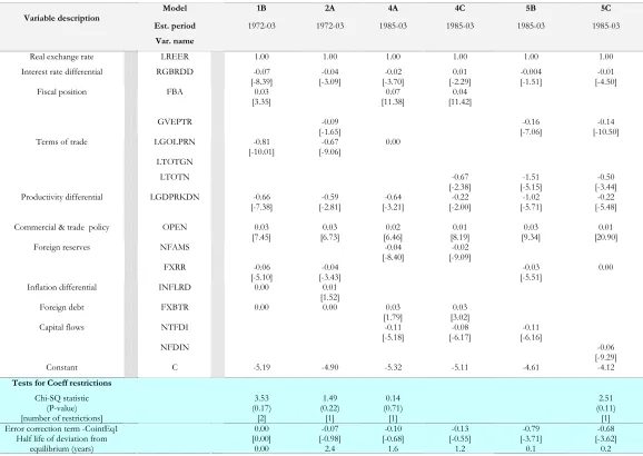
In the specifications labelled 1B and 2A, the vector equilibrium model was estimated using a sample of data spanning from the first quarter of 1972 to the last quarter of 2003. The specific combinations of variables examined are as follows:
o Model 1B consists of the real effective exchange rate of the rand (LREER), the real interest rate differential on the 10 year government bond between South Africa and the four major trading partners (RGBRDD), the fiscal deficit as a share of gross domestic product (FBA), the real US dollar gold price (LGOLPRN), the relative real gross domestic product per capita between South Africa and the four major trading partners (LGDPRKDN), total trade as a ratio of gross domestic product (OPEN), the total stock of gross foreign reserves as a ratio of gross domestic product (FXRR), the inflation rate differential between South Africa and the four major trading partners (INFLRD), and the stock of foreign debt measured as a ratio of gross domestic product (FXBTR).
o Model 2A distinguishes 1B by examining the influence of the fiscal variable in terms of the share of total government expenditure in gross domestic product (GVEPTR)
Regarding specifications 4A, 4C, 5B and 5C, these were estimated using data from 1985q1 through to 2003q4, partly to assess the robustness of the model, and also to examine the influence of the capital flows variable, whose data at the quarterly frequency is available only from 1985. The particular variables included in each model are as follows.
o Model 4C employed the same variables as in 4A, but the term of trade variable was assessed in term of LTOTN, the ratio of export to import prices excluding gold price.
o Model 5B has the same order of variables as 4C, but the fiscal variable in now examined in terms of GVEPTR, the ratio of total government expenditure to GDP, and the foreign reserves variable employed is FXRR, the total stock of gross reserves as a percentage of GDP.
o Finally, in model 5C, the influence of the capital flows variable is assessed in terms of the ratio of net foreign direct investment to gross domestic product (NFDIN).
In estimating these VECM specifications of the empirical model, both the nature of the intercept and trend, and the lag structure in the underlying VAR model had to be ascertained. In the case of trend specification, we chose option three of the five trend case assumptions discussed previously, which restricts the intercept seeing that our data is not trended but appear to fluctuate around a non-zero mean. With regard to the order of the VAR, we included four lags of each variable in their first differences as our analysis employs quarterly data12. Also included in the specifications are three seasonal
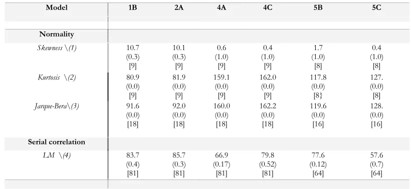
dummies (SR1, SR2, & SR3) which are meant to control for the effects of seasonality in the data. We tested for the appropriateness of this lag structure using the chi-square statistic for the wald test for joint lag exclusion, testing the null hypothesis that the lags are jointly not significantly different from zero, which, if accepted, implies that the lags should be excluded. The results of this lag exclusion test, presented in table 3-2, show that this null hypothesis is not supported by the data, suggesting that the lag structure is appropriate.
We also examined a number of the models’ diagnostics so as to assess the statistical adequacy of our model’s specifications. Table 3-3 presents chi-square statistics on testing
12