A Composite Weight based Multiple Attribute Decision Support System for the Selection of Automated Guided Vehicles

A Composite Weight based Multiple Attribute Decision

Support System for the Selection of Automated uided

Vehicles

Vishram B. Sawant

Government College of Engineering, Vidyanagar, Karad, 415124, Maharashtra, India.

Suhas S. Mohite

Government College of Engineering, Vidyanagar, Karad, 415124, Maharashtra, India.

ABSTRACT

This paper proposes a decision support system which integrates the objective weights of importance of the attributes as well as the subjective preferences of the decision maker to decide the composite weights of importance of the attributes. Using fuzzy set theory the qualitative attributes are converted into the quan-titative attributes. Based on this model, a decision support sys-tem AGVSEL is developed for the selection of AGVs. AGVs are ranked by using the technique for order preference by sim-ilarity to ideal solution (TOPSIS), block TOPSIS and modified synthetic evaluation method (M-TOPSIS). The effectiveness of the support system is demonstrated with an illustrative exam-ple. The computational results obtained enable evaluation and selection of an appropriate AGV. Sensitivity analysis reveals that at a moderate value of interpolating factor rank transition takes place for topmost position thereby achieving better insight into the complex interplay of subjective and objective weights. Fi-nally, the results of the proposed approach are compared with the results obtained by published methods. Thus, the proposed weight method with AGVSEL system improves decision mak-ing in MADM environment.

Keywords:

Multiple attribute decision making, automated guided vehicle, decision support system, TOPSISifx

1. INTRODUCTION

AGVs are battery-powered, unmanned vehicles with program-ming capabilities for path selection and positioning. They are capable of responding readily to frequently changing transport patterns and they can be integrated in fully automated manu-facturing systems. These features make AGVs a viable alter-native to other material handling methods. On the assumption that the labor costs will rise even more sharply in the future, AGVs will increase productivity, and improve system flexibility. The increasing interest in AGVs is reflected in the sales figures which reached a new peak in 2006 with a volume of $281.7 mil-lion according to a yearly survey among European AGV produc-ers carried out by the Department of Planning and Controlling of Warehouse and Transport Systems, Leibniz University Han-nover, Germany [1]. AGV applications can be found throughout all industrial branches, from the automotive, printing, pharma-ceutical sectors, metal, food processing to aerospace and port facilities.

An effective selection among more than 76 AGV manufactur-ers and different AGV models available in market requires the consideration of many quantitative and qualitative attributes. An MADM method is a procedure that specifies how attribute

infor-mation is to be processed in order to arrive at a better choice. AGV selection attribute is defined as a factor that influences the selection of an AGV for a given application. These attributes include: costs involved, floor space requirements, load carry-ing capacity, travel speed, lift height, turncarry-ing radius, travel pat-terns, programming flexibility, labor requirements, expandabil-ity, ease of operation, maintenance aspects, payback period, re-configuration time, hardware targebility, support for modular-ity (i.e. ease of integrating with FMS, ASRS, and robots), ro-bustness etc. AGV manufacturers develop AGVs of a variety of types and sizes. One company does not cover all niches equally well. Therefore, it is wise to evaluate AGVs based on a num-ber of attributes. The decision making process in the selec-tion of AGV consists of a combinaselec-tion of a variety of multi-dimensional attributes (see, Fig. 1). It includes: performance parameters, technical specifications, economical considerations and future expansion issues. One company does not cover all attributes equally well. Therefore, it is wise to evaluate AGVs based on a number of attributes.

To help address the issue of effective evaluation and selection of AGVs, various mathematical and systems modeling approaches have been proposed. The development of an intelligent mate-rial handling equipment selection system called matemate-rial han-dling equipment selection advisor (MHESA) is described in [2]. In addition to above, [3] developed decision support system for the selection of material handling equipments (SEMH). SEMH searches its knowledge base to recommend the type of mate-rial handling equipment to be used based on various charac-teristics like type, weight, size, etc. FUMAHES-fuzzy multi-attribute material handling equipment selection system consists of a database and a rule-based system [4]. In other applica-tion,[5] focused on the application of the AHP technique in selecting the optimal material handling equipment for a spe-cific material handling equipment. AHP - PROMETHEE inte-grated approach for selection of the most suitable equipment used by [6]. A decision support system to help the decision makers in their machining center selection decisions was devel-oped by [7]. One of the recent study proposed by [8], An inte-grated fuzzy multi-criteria decision making methodology for ma-terial handling equipment selection problem MHESP. The pro-posed methodology is based on fuzzy sets, Analytic Network Process (ANP) and Preference Ranking Organization METHod for Enrichment Evaluations (PROMETHEE) approaches. A new methodology for multi-attribute selection of automated guided vehicle (AGV) for the material handling. A modified grey rela-tional analysis (M-GRA) method combined with AHP has been used for selection of AGVs [9].

systematic and self-sufficient support system to guide the user or-ganizations in taking a decision in selecting a AGV. To the best of our knowledge, there is no decision making system that has been developed specifically for AGV selection considering available AGVs in the market. So also, different decision makers might assign different weights to different attributes; however, none of these systems provide the means for the user to select their own weightings on basis of subjective and objective information in-tegration. The proposed system in this paper, namely AGVSEL (AutomatedGuidedVehicleSELection), overcomes above lim-itations. It also uses crisp (non-fuzzy) and fuzzy MADM ap-proaches which take into account the uncertainties and impreci-sion that may be associated with the deciimpreci-sion making approach. The aim of the present paper is to propose a new MADM method where, composite weight is computed by integrating the ob-jective and subob-jective weights obtained by Shannon’s entropy method and Satty’s analytic hierarchy process (AHP) with differ-ent versions of TOPSIS. Fuzzy set theory can be utilized to cover the vagueness inherent in the nature of this selection problem. Experts express their judgments on the value of each alternative with respect to defined attribute in linguistic terms. This helps the model to be more user friendly and realistic. The remain-der of this paper is organized as follows: Section 2 describes the composite weight MADM method. Section 3 presents the pro-posed structure of developed DSS using TOPSIS/B-TOPSIS/M-TOPSIS methodologies. An illustrative example are considered for the AGV selection with results and validation in Section 4. Finally, conclusion and future studies are provided in Section 5.

2. PROPOSED MADM METHODOLOGY

The proposed MADM methodology is divided in to various steps as described below:

Step 1:Identify the goal; find out all possible alternatives,

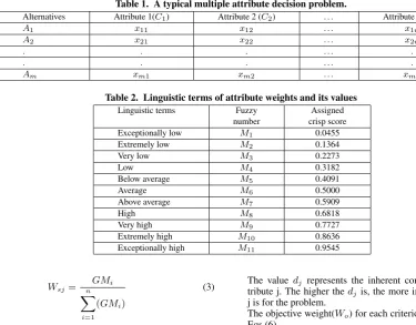
se-lection attribute and its measures for the given application. An MADM problem with finite possibilities can be concisely ex-pressed in matrix format as shown in Table 1. In this Table,A1, A2, . . . ,Am are possible alternatives among which decision

makers have to choose best alternative,C1,C2, . . . ,Cnare

at-tribute with which alternative performance are measured,xijis

the rating of alternative i with respect to attribute j, i = 1,2. . . ,m; j = 1,2. . . ,n;

Step 2:The process of transforming attributes value into a range

of 0-1 is called normalization and it is required in MADM to transform performance rating with different data measurement unit in a decision matrix into a compatible unit. The attributes are of two types, beneficial (i.e. higher values are desired) and non-beneficial (i.e. lower values are desired). The values associ-ated with the attributesxijmay be in different units (e.g., AGV

cost expressed in dollars, Load capacity expressed in Kg, etc.). The values of attributes can be normalized using the following equation: The normalized decision matrix is constructed using Eq.(1).

rij= xij q

Pn

j=1x 2

ij

(1)

whererijis the normalized value obtained from decision matrix.

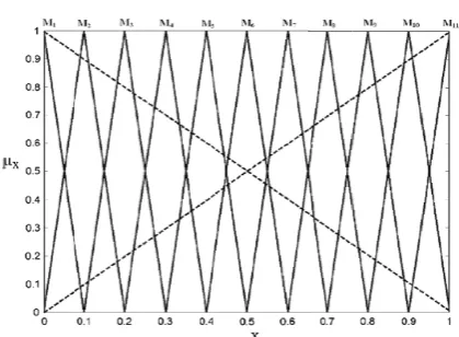
It may be added here that Eq.(1) can deal with quantitative at-tributes. However, there exists some difficulty in the case of qualitative attributes (i.e. quantitative value is not available). A ranked value judgment on a fuzzy conversion scale is proposed in this paper by using fuzzy set theory. This approach is based on the work of [10]. The presented numerical approximation sys-tem syssys-tematically converts linguistic terms to their correspond-ing fuzzy numbers. An 11-point scale is proposed in this paper for better understanding and representation of the qualitative at-tribute. Table 2 represents the selection attribute on a qualitative scale using fuzzy logic, corresponding to the fuzzy conversion

Selection of AGV Model

Performance parameters Technical specifications Economical considerations Future Expansion

-Max. Load capacity -Battery charging time - Max. Lift height -Length, width, height - Travel speed

-Maintenance -Convenience -Travel patterns -Programming Flexibility -Purchasing cost (Equipment cost, tax, salvage cost, etc) -Operating cost

-Hardware targebility - Support for modularity (i.e. interface with FMS, ASRS, and Robots. -Robustness etc       Level 1:   Goal  Level 2:   Attributes  Level 3:   Sub‐attributes  Level 4: 

Alternatives  ………

Fig. 1. Hierarchical structure of selecting AGV in AGVSEL system.

  Fig. 2. Linguistic terms to fuzzy numbers conversion (11-point

scale).

scale as shown in Fig.2. The list of possible fuzzy numbers that can be assigned in weighting the attributes and their linguistic correspondences are provided in Table 2.

Step 3:Determination of weights of importance of the attributes

In the following steps the subjective and objective weight com-putation procedure incorporated in AGVSEL system is pro-posed.

Step 3.1:Subjective weights of importance of the attributes

The steps for the calculation of subjective weights (Ws) are

enu-merated below.

First compute the relative importance of different attributes with respect to the objective. To do so, one has to construct a pair-wise comparison matrix using a scale of relative importance. The judgments are entered using the fundamental scale of the analytic hierarchy process(AHP) as given in Table 3 [11,12]. An attribute compared with itself is always assigned the value 1 so the main diagonal entries of the pair-wise comparison matrix are all 1. The numbers 3, 5, 7, and 9 correspond to the verbal judg-ments moderate importance, strong importance, very strong im-portance, and absolute importance (with 2, 4, 6, and 8 for com-promise between the previous values).

Next, the relative normalized weight(Wj)of each attribute by

(i) calculating the geometric mean of ith row and (ii) normalizing the geometric means of rows in the comparison matrix. This can be represented as

GMi=

( n

Y

j=1 aij

)1/n

Table 1. A typical multiple attribute decision problem.

Alternatives Attribute 1(C1) Attribute 2 (C2) . . . Attribute n (Cn)

A1 x11 x12 . . . x1n

A2 x21 x22 . . . x2n

. . . .

. . . .

Am xm1 xm2 . . . xmn

Table 2. Linguistic terms of attribute weights and its values

Linguistic terms Fuzzy Assigned

number crisp score

Exceptionally low M1 0.0455

Extremely low M2 0.1364

Very low M3 0.2273

Low M4 0.3182

Below average M5 0.4091

Average M6 0.5000

Above average M7 0.5909

High M8 0.6818

Very high M9 0.7727

Extremely high M10 0.8636

Exceptionally high M11 0.9545

Wsj= GMi n X

i=1

(GMi)

(3)

The geometric mean method of AHP is used in the present work to find out the relative normalized weights of the attributes be-cause of its simplicity and easiness to find out the maximum Eigen value and to reduce the inconsistency in judgments. Calculate matrix A3 and A4 such that A3 =AnxnX A2 and A4

= A3/A2, where A2 =Wsj= [W1,W2, . . .Wn]T.

Find out the maximum Eigen valueλmaxthat is the average of

matrix A4.

Consistency Test: Calculate the consistency index CI = (λmax− N)/(N −1). The smaller the value of CI, the smaller is the deviation from the consistency. Obtain the random index (RI) for the number of attributes used in decision making. The reference RI values for different numbers of N are shown in Table 4. Calculate the consistency ratio: CR=CI/RI. A value of CR of 0.1 or less is considered as acceptable and decision is taken for preparation of the judgment matrix otherwise the necessary changes are made while preparation of the judgment matrix.

Step 3.2:Objective weight calculation procedure

Shannon’s entropy is a well known method for obtaining the ob-jective weights for a MADM problem especially when obtaining a suitable weight based on the preferences are not possible. The procedure of Shannon’s entropy can be expressed in a series of steps for the calculation of objective weights (Wo) as per

follow-ing steps given in [13].

First the normalized decision matrix is constructed using Eq.(1). After normalizing the decision matrix, the entropy valuesejare

calculated using Eq.(4).

ej=−k n X

j=1

rijlnrij (4)

where k is a constant, k =(ln(n))−1_{(n indicates number of} de-cision alternatives). The degree of divergencedjof the intrinsic

information of each attrubute (j = 1,2, . . . ,n) may be calculated as

dj= 1−ej (5)

The valuedj represents the inherent contrast intensity of

at-tribute j. The higher thedjis, the more important the attribute

j is for the problem.

The objective weight(Wo) for each criterion can be obtained by

Eqs.(6).

Woj= dj

pPn

k=1dk

(6)

Step 3.3:Composite weights of importance of the attributes The

weights obtained by subjective and objective methods are dif-ferent and so also the ranking. If the decision maker models seamlessly subjectivity of DM’s expertise and objectivity of at-tribute data then decision maker may use the composite weights described by the equation (7). The equation gives combination of subjective and objective weight spectrum.

Wcj= [βWsj+ (1−β)Woj] (7)

whereWcjis the composite weight of jth attribute andWsjand Woj are the subjective and objective weights.β is composite

weight coefficient and the values are between 0 and 1 with an interval of 0.1. For subjective approach, S-100%,β= 1;Wcj= Wsj, For objective approach O-100%,β= 0;Wcj=Woj, and

Pn

c=1Woj= 1; 0≤β≤1.

Step 4:Computation of AGV selection index (ASI)

TOPSIS/B-TOPSIS/M-TOPSIS methods are used for computa-tion of ASI. TOPSIS one of the classical MADM methods was developed by Hwang and Yoon [10], B-TOPSIS by Shanian and Savadogo [14] and M-TOPSIS advocated by [15,16] are used to get ASI to rank AGVs using crisp/fuzzy MADM approaches.

ASI by TOPSIS method.The reasons for choosing TOPSIS are

that (1) the TOPSIS approach is rational and easy to compre-hend, (2) the computations involved are simple. The steps of the fuzzy TOPSIS approach are presented by [17].

ASI by B-TOPSIS method.The block(B) TOPSIS method is a

simplified version of TOPSIS, the two euclidean distances ideal and negative ideal solutions for each alternative are, calculated as: The distance of a alternativejto the positive ideal solution (D_i+), and from the negative ideal solution (D_i−) are calculated using Eqs. (2) and (3) given below by [14].

D_i+= m X

j=1

Table 3. Relative importance of attributes (aij)

Relative importance (aij) Description

1 Attributes i and j are equally important

3 Attribute i is moderately more important than attribute j

5 Attribute i is strongly more important than attribute j

7 Attribute i is very strongly more important than attribute j

9 Attribute i is absolutely more important than attribute j

2,4,6,8 Intermediate values of relative importance

Table 4. Random Index (RI) values for corresponding matrix size (Saaty 2004).

Attributes (n) 1 2 3 4 5 6 7 8

RI values 0 0 0.52 0.89 1.11 1.25 1.35 1.40

D−i = m X

j=1

|vij−vj−|;i= 1,2, ...., n;j= 1,2, ...., m; (9)

Wherevijare weighted normalized values andvj+,v − j are the

positive ideal and negative ideal solutions.

ASI by M-TOPSIS method.M-TOPSIS is a method sourced

from TOPSIS. Of the two methods which are discussed above, we believe that the M-TOPSIS is more reasonable because the ranking order of alternatives was determined by their distances to optimized ideal reference point. Also, equation to calculate ASI of M-TOPSIS is more accurate than equation of TOPSIS/B-TOPSIS. It can solve the problems of TOPSIS/B-TOPSIS such as rank reversals and evaluation failure when alternatives are symmetrical [17].

Step 5:Ranking and final selection of AGV. A final decision is

taken keeping in view of the attribute data supplied by the indus-try. All possible constraints likely to be experienced by the DM are looked in during this stage. These include constraints such as maximum load to be carried, maximum lift height, maximum Travel speed, budgetary provision. However, compromise may be made in favor of an alternative with a higher value of ASI. In the next section, we present the structure of the decision support system - AGVSEL.

3. STRUCTURE OF THE DECISION SUPPORT

SYSTEM - AGVSEL

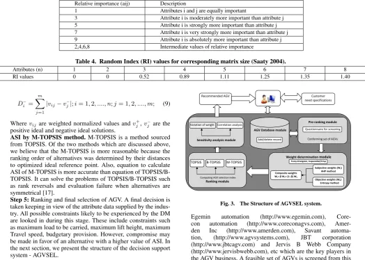
In the development of AGVSEL, the attributes have been hier-archically structured in four levels (see, Fig. 1), in accordance with the MADM framework. The level 1 contains the overall objective for AGV selection. Level 2 consists of four groups of attributes. Level 3 contains the detailed attributes under each of the above groups. Level 4 contains the list of AGVs available in market. The developed decision support system incorporates five separate modules (see, Fig. 3), namely, database module, pre-ranking module, weight determination module, pre-ranking module and analysis module. Pre-ranking module prompts the user to answer 16 questions to eliminate the non confirming AGVs and obtain a feasible set of AGVs. The feasible sets of AGVs are then ranked by TOPSIS/B-TOPSIS and M-TOPSIS methods. The en-tire system has been developed in a software program using Vi-sual Basic in Windows environment. Details of the modules are described in the following sections.

3.1 Database module

This module comprises of AGV database of 114 AGVs from 76 manufacturers worldwide. One can add or delete a new AGV in the AGVSEL system database. In devel-oped system, the database includes different attributes (see, Fig. 1). There was no information available about attribute data in published literature for AGV selection. However, to fill this gap the data was taken from online mode, viz.,the HK Systems (http://www.hksystems.com),

                                                                         AGV Database module Customer  need specifications 

      Weight determination module                                           Pre‐ranking module  

Conforming set of AGVs 

      Computing AGV selection index  

Ranking module            Sensitivity analysis module 

Subjective weights (Ws) AHP method 

Objective weights (Wo)

   Entropy method 

Composite weights Wc= β Ws+ (1‐ β) Wo  Recommended AGV 

TOPSIS  B‐TOPSIS  M‐TOPSIS 

 Add/delete record Variation of weight  Correlation analysis 

Questionnaire for screening

   Fuzzy‐triangular, trapezoidal/Crisp 

Fig. 3. The Structure of AGVSEL system.

Egemin automation (http://www.egemin.com), Core-con automation (http://www.coreconagvs.com), Amer-den Inc (http://www.amerden.com), Savant automa-tion, (http://www.agvsystems.com), JBT corporation (http://www.jbtcagv.com) and Jervis B Webb Company (http://www.jervisbwebb.com), etc which are the key players in the AGV business. A feasible set of AGVs is screened from this extensive database using the pre-ranking module described in the next section.

3.2 Pre-ranking module

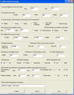
The pre-ranking module of the AGVSEL, (see, Fig.4) poses a questionnaire to the decision maker with answers. The user has the choice to answer suitable number of questions. The minimum and maximum values of load to be moved are entered in response to the first question. The transport unit size, i.e., length, width and height, transport units that will make up the goods to be transported, distance to be travelled, available floor-space, bud-get allocated, etc., are entered through questions 2 to 7. The num-ber of pick-up and drop-off points, maximum lift height, mini-mum turning radius, labor requirements are entered in questions 8 to 11. Question 12 to 16 calculate the expansion in near future, battery charging details, reconfiguration time, any particular en-vironmental conditions to be taken into account, or any other in-formation user wants to provide can be entered in response to this questions. Once the broad specifications are entered by the deci-sion maker in the pre-ranking module, the feasible set of AGVs are determined by this module and is provided on the console (see, Fig. 5). The feasible set can be simultaneously passed on to the weight determination procedure as discussed in section 2 step 3 for assigning weights.

3.3 Ranking module

TOPSIS/B-Fig. 4. Pre ranking module of AGVSEL.

Fig. 5. output screen of AGVSEL system for the pre ranking module

TOPSIS/M-TOPSIS ranking methods are used for ranking feasi-ble AGVs. In the following section the ranking methods used in AGVSEL system are briefly discussed.

3.3.1 AGV selection index by TOPSIS method. The reasons of choosing TOPSIS are that (1) the TOPSIS approach is rational and easy to comprehend, (2) the computations involved are sim-ple, (3) the concept allows both subjective and objective weights to be aggregated in the decision-making process. The readers can referred to [10,17] for detailed explanations and applicational steps of crisp/fuzzy TOPSIS approach.

3.3.2 AGV selection index by B-TOPSIS method. The block(B) TOPSIS method is a simplified version of TOPSIS, the two euclidean distances ideal and negative ideal solutions for each alternative are, calculated as: The distance of a alternativej

to the positive ideal solution (D_i+), and from the negative ideal solution (D−_i) are calculated using Eqs. (2) and (3) given below by [14].

D+_i = m X

j=1

|vij−v+j|;i= 1,2, ...., n;j= 1,2, ...., m; (10)

Di−= m X

j=1

|vij−v−j|;i= 1,2, ...., n;j= 1,2, ...., m; (11)

Wherevijare weighted normalized values andvj+,v − j are the

positive ideal and negative ideal solutions.

3.3.3 AGV selection index by M-TOPSIS method. M-TOPSIS is a method sourced from TOPSIS. Of the two methods discussed above, we believe that the M-TOPSIS is more reasonable be-cause the ranking order of alternatives was determined by their distances to optimized ideal reference point [16]. Also, equation to calculate index value of M-TOPSIS is more accurate than equation of TOPSIS/B-TOPSIS. It can solve the problems of TOPSIS/B-TOPSIS such as rank reversals and evaluation failure when alternatives are symmetrical. The ranking obtained with TOPSIS/B-TOPSIS methods are compared with M-TOPSIS for validation purpose and to check consistency in ranking.

3.4 Analysis module

In the analysis module, the user enters the subjective weights directly as crisp/fuzzy numbers (see, Fig. 6) and calculates the consistency ratio. The ratio value of 0.1 or less is considered as acceptable as it reflects an informed judgment that could be at-tributed to the knowledge of the DM about the problem under study. The rankings are then obtained for each set of weights us-ing TOPSIS/B-TOPSIS/M-TOPSIS methods. An example of the output screen by using TOPSIS method is provided in Fig. 6. In the output screen, the feasible AGVs are listed according to their ranking scores. The user can see the ranking scores and techni-cal specifications in the same screen. We can also obtain ranking of AGVs by clicking on nine different sets of combinations of subjective and objective weights (see, Fig. 6). The correlation analysis can also be carried out to test the accuracy of rankings obtained. In the next section, we present results for the AGV selection index calculations by considering industrial case. The results are presented for variation composite weights followed by a brief discussion.

4. RESULTS AND DISCUSSIONS

4.1 AGV selection using quantitative data

An AGV selection example using quantitative data for a manu-facturing enterprise in Maharashtra, India is presented using the developed AGVSEL system.

Step 1:The requirements and attribute information of the AGVs

Table 5. Information about the AGV from industry.

Specifications Values

Maximum load to be carried (MLC): 3600 kg (3.6 tons)

Maximum lift height (MLH): 150 mm

Battery should not get discharge before : 4 hrs

Maximum budgetary provision: $20,000

Maximum Travel speed (MS): High

Length of AGV (L): High

Width of AGV (W): High

Height of AGV (H): High

Purchasing cost (PC): Low

Position accuracy (P): High

Table 6. Comparision of the attribute weights for AGV selection.

Methods SW OW CW IW CombineW PW

Attributes [11,12] [13] [18] [19] [20] β= 0.5

L 0.072 0.092 0.059 0.042 0.081 0.080

W 0.072 0.087 0.056 0.045 0.079 0.076

H 0.072 0.113 0.073 0.035 0.090 0.075

MLC 0.170 0.214 0.325 0.043 0.191 0.192

MS 0.092 0.109 0.090 0.046 0.100 0.101

B 0.170 0.015 0.022 0.619 0.090 0.092

P 0.151 0.117 0.158 0.070 0.133 0.134

LH 0.104 0.085 0.079 0.067 0.094 0.095

LS 0.092 0.163 0.134 0.031 0.123 0.128

SW-Subjective weights, OW-Objective weights, CW-Compromised weighting method, IW-Integrated weight method, CombineW-Combined weight method, PW-proposed weight method.

Fig. 6. Input screen for the weights in the weight decision module.

Step 2:The values of the attributes are normalized using Eq. (1)

and are not shown here due to space constraint.

Step 3:Next, subjective weights (by AHP method) explained in

step 3.1 are calculated with the DM’s expertise (see, Table 6). The consistency ratio of the pairwise comparison matrix is cal-culated to be 0.0487. The ratio value of 0.1 or less is considered as acceptable as it reflects an informed judgment of the DM and weights obtained are used in the selection process. The objective weights are calculated by using entropy method as explained in step 3.2. The composite weights of importance of the attributes

Fig. 7. output screen for the spearmans rank correlation test.

are computed using Eq.(8) for different composite weight coef-ficient (β) and the values are between 0 and 1 with an interval of 0.1. It may be mentioned here that forβ= 1, the composite weights are same as that of subjective weights of step 3.1 and for andβ= 0, the composite weights are same as that of ob-jective weights of step 3.2. We found that in case of subob-jective weights i.e.β=1, the attributes MLC, L, W and battery capacity have higher weight values compared to other attributes. So also, the attributes H, LS has higher weight values compared to MS, P, LH. It is known from MADM theory that, the attributes having lower weights have no major effect on the final selection.

Step 4:Computation of AGV selection index (ASI) and the

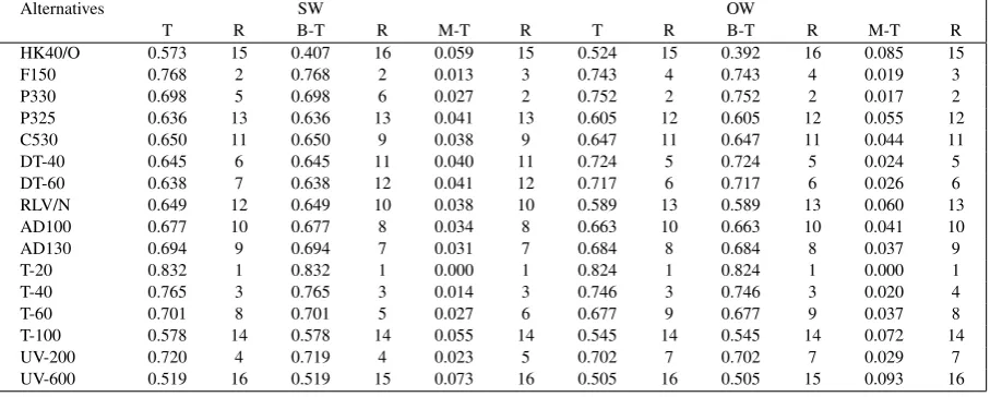
Table 7. AGV selection index, rank(R) using TOPSIS(T), B-TOPSIS(B-T), M-TOPSIS(M-T) for subjective(SW) and objective weights(OW).

Alternatives SW OW

T R B-T R M-T R T R B-T R M-T R

HK40/O 0.573 15 0.407 16 0.059 15 0.524 15 0.392 16 0.085 15

F150 0.768 2 0.768 2 0.013 3 0.743 4 0.743 4 0.019 3

P330 0.698 5 0.698 6 0.027 2 0.752 2 0.752 2 0.017 2

P325 0.636 13 0.636 13 0.041 13 0.605 12 0.605 12 0.055 12

C530 0.650 11 0.650 9 0.038 9 0.647 11 0.647 11 0.044 11

DT-40 0.645 6 0.645 11 0.040 11 0.724 5 0.724 5 0.024 5

DT-60 0.638 7 0.638 12 0.041 12 0.717 6 0.717 6 0.026 6

RLV/N 0.649 12 0.649 10 0.038 10 0.589 13 0.589 13 0.060 13

AD100 0.677 10 0.677 8 0.034 8 0.663 10 0.663 10 0.041 10

AD130 0.694 9 0.694 7 0.031 7 0.684 8 0.684 8 0.037 9

T-20 0.832 1 0.832 1 0.000 1 0.824 1 0.824 1 0.000 1

T-40 0.765 3 0.765 3 0.014 3 0.746 3 0.746 3 0.020 4

T-60 0.701 8 0.701 5 0.027 6 0.677 9 0.677 9 0.037 8

T-100 0.578 14 0.578 14 0.055 14 0.545 14 0.545 14 0.072 14

UV-200 0.720 4 0.719 4 0.023 5 0.702 7 0.702 7 0.029 7

UV-600 0.519 16 0.519 15 0.073 16 0.505 16 0.505 15 0.093 16

Table 8. Rankings of the AGV models by different weight generation methods.

AGVs T B-T M-T

PW CombineW CW IW PW CombineW CW IW PW CombineW CW IW

HK40/O 15 15 12 15 15 16 12 15 16 15 12 15

F150 3 3 3 6 3 3 3 6 2 3 3 6

P330 4 2 2 16 2 2 2 16 4 2 2 16

P325 12 13 14 1 13 13 14 1 12 13 14 1

C530 11 11 13 2 11 11 13 2 11 11 13 2

DT-40 6 6 6 11 6 6 6 11 6 6 6 11

DT-60 7 9 7 12 8 9 7 12 9 8 7 12

RLV/N 13 12 8 5 12 12 8 5 13 12 8 5

AD100 10 10 10 4 10 10 10 4 10 10 10 4

AD130 8 8 9 3 9 8 9 3 8 9 9 3

T-20 1 1 1 7 1 1 1 7 1 1 1 7

T-40 2 4 4 9 4 4 4 9 3 4 4 9

T-60 9 7 11 10 7 7 11 10 7 7 11 10

T-100 14 14 15 13 14 14 15 13 14 14 15 13

UV-200 5 5 5 8 5 5 5 8 5 5 5 8

UV-600 16 16 16 14 16 15 16 14 15 16 16 14

ascending order of their selection index for M-TOPSIS method. It can be seen that the match between the TOPSIS, B-TOPSIS and M-TOPSIS method is very good and is confirmed by Spear-man’s test.

Step 5:The obtained ranking is discussed with the customer so

as to ascertain the suitability amongst the top three alternatives. It was found that these alternatives conform with the desired spec-ifications to a great extent. The AGV model T-20 can be consid-ered the best choice as determined by TOPSIS, B-TOPSIS, and M-TOPSIS methods respectively and AGV UV600 is the last choice of the decision maker for a given application.

4.2 Effect of composite weights

Next, the effect of proposed composite weights on final ranking is discussed here. The top ranked AGV using TOPSIS method is T-20 forβranging from 0 to 1.0 at an interval of 0.2. Rank transition is observed for second position between P-330 to T-40 with the variation inβ(see, Table 8), in case of B-TOPSIS method T-20 remains at top but second position is occupied by P-330 forβranging from 0 to 0.2, T40 forβranging from 0.3 to 0.4 and F-150 forβranging from 0.4 to 1.0, followed by T-40, F-150 for third rank (see, Table 8). T-20 remains at top if we rank feasible AGVs using M-TOPSIS method second position is occupied by P-330 and third position by F-150 (see, Table 8). In general, it does not matter that the different methods give differ-ent rankings, so long as the first choice AGV is consistdiffer-ent. The

results obtained provide valuable insight into the rank transition taking place with the variation in composite weight caused by β. The results are indicative of the fact that selection of the best AGV from the feasible set not only depends on ranking method but also on the interpolating weight factorβ. In this illustration, top three AGV are T-20, P-330 and T-40 are the best choices and don’t need further scrutiny with respect to their specifications and these AGVs can be selected for the given application. Thus, this system helps DM’s to visualize the changes in the ranking of AGV withβ. The system quickly and efficiently simulates ”‘what if?” scenario for different composite weights and helps in developing insight into the complex interplay of composite weights. The AGVSEL system can be generalised so that it can consider any number of quantitative and qualitative fuzzy AGV selection attributes. Further, the it can be used for any other type of decision making situations as well with minor modifications in software code.

4.3 Validation of the proposed method

differ-ent sets of attribute weights are shown in Table 8. We found that the weights of attributes obtained by the four methods are differ-ent, particularly combined weight method and proposed compos-ite weight method give similar weights. So also the rankings of the 16 AGV alternatives derived by the combined weighting and proposed composite weight model are very close but,they are not similar in case of compromised weighting method and integrated weight method. While it is natural that different approaches will usually lead to different results in a multiple attribute decision making problem and the adoption of a specific approach is up to the decision maker’s preference and the decision environment. Through the above examination and analyses,it can be summa-rized that the proposed weight method has the following advan-tages: The weights of attributes determined using the proposed method are more comprehensive and convincing as these are obtained by interpolating subjective and objective weights. The proposed method not only incorporates the amount of informa-tion each attribute contains but, also DM’s subjective preferences while calculating weights. The rank transition taking place be-tween different alternatives is visible and this effect can be mod-elled with proposed composite weight model.

4.4 Consistency in ranking using Spearman’s test

The statistical significance of the difference between the ranking obtained for the TOPSIS approach and for the B-TOPSIS/M-TOPSIS approach is determined using Spearman’s rank-correlation test. This test is a special form of correlation test used when the actual values of paired data are substituted with the ranks which the values occupy in the respective sam-ples. In this study, Spearman’s test evaluates the similarity of the rankings of the AGVs using TOPSIS and B-TOPSIS/M-TOPSIS methods. In the application of Spearman’s test, to test the null hypothesis (H0: There is no similarity between the two rank-ings), a test statistic, Z, is calculated using Eqs. (12) and (13) and compared with a pre-determined level of significance value.

rs= 1− 6

k X

j=1

(dj)2

K(K2₋₁₎ (12)

Z=rs

√

K−1 (13)

In this study, 1.645, which corresponds to the critical Z value at the level of significance ofα= 0.05, is selected. If the test statis-tic computed by Eq. (13) exceeds 1.645, the null hypothesis is rejected and it is to be concluded thatH1: The two rankings are similar is true. In Eqs. (12) and (13),djis the ranking difference

of alternativesj, andkis the number of alternatives to be com-pared.rsrepresents the Spearman’s rank correlation coefficient

in Eqs. (12) and (13). The rankings obtained by the TOPSIS, B-TOPSIS and M-B-TOPSIS in the AGV selection problem are pro-vided in Fig. 6. The Spearman rank correlation coefficient be-tween the methods is 0.8930 and 0.8790 which shows high cor-relation between the rankings proposed by the two methods. The comparison is performed by taking the difference of the ranks of the TOPSIS, B-TOPSIS and M-TOPSIS, and then calculating Spearman’s correlation coefficient (Z-value) for the difference. The calculated Z-value, 3.850, is higher than 1.645, which im-plies that the difference in the two ranking results is statistically insignificant. Based on the test results, it is concluded that the rankings obtained by the test are realistic.

5. CONCLUSIONS

The composite weight based MADM method presented in this paper is incorporated in the decision support system (AGVSEL). It provides the decision maker a great deal of flexibility to com-bine subjective and objective weights in terms of weighting

fac-torβand arrive at rank. The effectiveness of the method is ex-amined with an illustrative example of selection of AGV for an industrial application. The incorporation of decision makers knowledge and database of most AGV models available in mar-ket into the support system has made the AGVSEL more com-prehensive. The system quickly and efficiently simulates ”‘what if?” scenario for different composite weights and helps in devel-oping insight into the complex interplay of subjective and objec-tive weights. In example, the AGV model T-20 can be considered as the best choice as determined by TOPSIS, B-TOPSIS, and M-TOPSIS methods along spectrum of weights and AGV UV-600 is the last choice of the decision maker for a given application. The results obtained provide valuable insight into the rank transi-tion taking place at intermediate positransi-tion with the variatransi-tion ofβ. The Spearman rank correlation coefficient between the methods is 0.8930 and 0.8790 which shows high correlation between the rankings proposed by the methods. Validation of the proposed method at (β= 0.5) with the combined weight method [20], com-promised weighting method [18] and integrated weight method [19] shows T-20 as best choice and UV-600 as the last choice. Sensitivity analysis reveals that at moderate value of interpolat-ing factor (β) rank transition takes place for topmost position thereby achieving better insight into the complex interplay of subjective and objective weights.

6. REFERENCES

[1] Lothar S., Sebastian B., & Stefan B., Automated Guided Vehicle Systems: a Driver for Increased Business Perfor-mance In Proceedings of the International MultiConfer-ence of Engineers and Computer Scientists 2008 Vol II IMECS 2008.

[2] Chan F.T.S., Ip R.W.L., & Lau H., Integration of expert system with analytic hierarchy process for the design of material handling equipment selection system, Journal of Materials Processing Technology, (2001) 116:137-145. [3] Fonseca D.J., Uppal G.,& Greene T.J., A knowledge-based

system for conveyor equipment selection., Expert Systems with Applications, (2004) 26:615-623.

[4] Kulak O., A decision support system for fuzzy multi-attribute selection of material handling equipments., Expert Systems with Applications, (2005) 29:310-319.

[5] Chakraborthy S., & Banik D., Design of a material han-dling equipment selection model using analytic hierarchy process. The International Journal of Advanced Manufac-turing Technology, (2006) 28:1237-1245.

[6] Da˘gdeviren M., Decision making in equipment selection: an integrated approach with AHP and PROMETHEE. Jour-nal of Intelligent Manufacturing, (2008) 19:397-406. [7] I˙C¸ , Yusuf Tansel, & Yurdakul, M. Development of a

deci-sion support system for machining center selection., Expert Systems with Applications, (2009) 36:3505-3513. [8] Tuzkaya G., G˝ulsun B., Kahraman C., & Ozgen D., An

integrated fuzzy multi-criteria decision making methodol-ogy for material handling equipment selection problem and an application. Expert Systems with Applications, (2010) 37:2853-2863.

[9] Maniyaa K. D., and Bhatt M. G., A multi-attribute selection of automated guided vehicle using the AHP/M-GRA tech-nique. International Journal of Production Research, (2011) 49: 6107-6124.

[10] Hwang C.L. , Yoon K., Multiple Attribute Decision Making Methods and Applications, Springer, Berlin, Heidelberg, 1991.

[12] Saaty, T.L., How to make a decision: the analytic hierarchy process, Interfaces ,(1994) 24(6):1943.

[13] Shannon, C.E., & Weaver W., The Mechanical Theory of Communication., University of Illions Press, 1947. [14] Shanian A., & Savadogo O., TOPSIS multiple-criteria

de-cision support analysis for material selection of metallic bipolar plates for polymer electrolyte fuel cell. Journal of Power Sources, (2006) 159: 1095-1104.

[15] Deng H., Yeh C.H.,& Willis R.J., Inter-company compari-son using modified TOPSIS with objective weights. Com-puters and Operations Research, (2000) 27: 963-973. [16] Ren, L., Y. Zhang, Y.Wang & Z. Sun., Comparative

Anal-ysis of a Novel M-TOPSIS Method and TOPSIS, Applied Mathematics Research eXpress, (2007) Vol. 7, Article ID abm005, 10 pages, doi:10.1093/amrx/abm005.

[17] I˙C¸ , Yusuf Tansel, & Yurdakul, M., Development of a quick credibility scoring decision support system using fuzzy TOPSIS. Expert Systems with Applications, (2010) 37:567-574.

[18] Feng, C., & Chen, C., The determination of criteria weights compromised weighting method. Traffic and Transporta-tion, (1992) 14: 51-67.