Munich Personal RePEc Archive
Econometric estimation in long-range
dependent volatility models: Theory and
practice
Casas, Isabel and Gao, Jiti
Universidad Carlos III de Madrid, University of Adelaide
October 2006
Online at
https://mpra.ub.uni-muenchen.de/11981/
Econometric Estimation in Long–Range Dependent Volatility
Models: Theory and Practice
Isabel Casas1,2 and Jiti Gao2
1Department of Statistics and Econometrics, Universidad Carlos III de Madrid, C/Madrid,
126, 28903-Getafe (Madrid) Spain.
2School of Economics, The University of Adelaide, Adelaide SA 5005, Australia, and
School of Mathematics and Statistics, The University of Western Australia, Crawley WA
6009, Australia.
Abstract
It is commonly accepted that some financial data may exhibit long-range dependence, while other financial data exhibit intermediate–range dependence or short–range depen-dence. These behaviours may be fitted to a continuous–time fractional stochastic model. The estimation procedure proposed in this paper is based on a continuous–time version of the Gauss–Whittle objective function to find the parameter estimates that minimize the discrepancy between the spectral density and the data periodogram. As a special case, the proposed estimation procedure is applied to a class of fractional stochastic volatility models to estimate the drift, standard deviation and memory parameters of the volatility process under consideration. As an aplication, the volatility of the Dow Jones, S&P 500, CAC 40, DAX 30, FTSE 100 and NIKKEI 225 is estimated.
KEYWORDS: Continuous–time model, diffusion process, long–range dependence, stochas-tic volatility.
1. Introduction
There is a long history about the study of stochastic volatilities. More than thirty years ago, Black and Scholes (1973) assume a constant volatility to derive their famous option pricing equation. The implied volatility values obtained from this equation show skewness, suggesting that the assumption of constant volatility is not feasible. In fact, the volatility shows an intermittent behaviour with periods of high values and periods of low values. In addition, the asset volatility cannot be directly observed. Stochastic volatility (SV) models deal with these two facts. Taylor (1986) and Hull and White (1987) were amongst the first to study the logarithm of the stochastic volatility as an Ornstein– Uhlenbeck process. A review and comparative study about modeling SV up to 1994 has been given by Taylor (1994). Andersen and Sørensen (1996) examine generalized moments of method for estimating stochastic volatility model. Andersen and Lund (1997) extend the CIR model proposed by Cox, Ingersoll and Ross (1985) to associate the spot interest rate with stochastic volatility process through estimating the parameters with the efficient method of moments. The main assumption of the SV model is that the volatility is a log–normal process. The probabilistic and statistical properties of a log– normal are well known. However, parameter estimation has not been uncomplicated due to the difficulty finding the maximum likelihood (ML) function. The authors also like to mention the nonuniqueness of the log–normal distribution as reviewed by Stoyanov (2004). In addition to the log–normal distribution, Barndorff–Nielsen and Leonenko (2005) study other possible distributions of the volatility process, such as the Gamma and inverse Gaussian distributions. A recent review about the development of multivariate stochastic volatility is given in Asai, McAleer and Yu (2006).
Recent studies show that some data sets may display long–range dependence (LRD). See, for example, the recent surveys by Beran 1994, Baillie and King 1996, Anh and Heyde 1999, and Robinson 2003. Since about ten years ago, there has been some work on studying stochastic volatility with LRD. Breidt, Crato and De Lima (1998), Comte and Renault (1998), and Harvey (1998) were among the first to consider long–memory stochastic volatility (LMSV) models. Meanwhile, Breidt, Crato and De Lima (1998), and Harvey (1998) independently consider a LMSV case where the log–volatility is modelled as a fractionally integrated ARMA (ARFIMA) process. Comte and Renault (1998) consider a continuous–time fractionally stochastic volatility (FSV) model of the form
dY(t) = v(t) dB(t) and dx(t) =−αx(t)dt+σ dBβ(t), (1)
standard Brownian motion,α is the drift parameter involved in the stochastic volatility process, σ > 0 is the volatility parameter involved in the stochastic process, and Bβ(t)
is a fractionally Brownian motion process of the form: Bβ(t) = R0t (t−s)β
Γ(1+β)dB1(s), where
B1(t) is another standard Brownian motion and Γ(x) is the usual Γ function. A process
displays LRD if 0 < β < 12. When β = 0, the process is called short–range dependent. The process is called intermediate–range dependent if −12 < β <0 (see §12.4 of Brock-well and Davis 1990 for more precise definitions). Comte and Renault (1998) propose a discretization procedure to approximate the solution of their continuous–time FSV model. An estimation procedure for 0 < β < 1
2 is then developed for a discretized
ver-sion of the solution Y(t) based on the so–called log–periodogram regression. Recently, Deo and Hurvich (2001) also study such an estimation procedure based on the log– periodogram regression method, and then establish the mean–squared error properties as well as consistency results for an estimator of β using the so–called GPH estimator initially proposed by Geweke and Porter–Hudak (1983). Gao (2004) points out that it is possible to estimate all the parameters involved in model (1) using the so–called continuous–time version of the Gauss–Whittle contrast function method proposed in Gao, et al. (2001) and Gao, Anh and Heyde (2002). Other closely related papers in-clude Giraitis and Surgailis (1990), Hosoya (1997), Sun and Phillips (2003), Andrews and Sun (2004), Anh, Leonenko and Sakhno (2004), and Leonenko and Sakhno (2006).
This paper considers a class of stochastic volatility models of the form
dY(t) = V(t) dB(t) (2)
with V(t) being given by V(t) = eX(t), in which
X(t) =
Z t
−∞A(t−s) dB1(s), (3)
where A(·) is a deterministic function such that X(t) is stationary, and the explicit expression ofA(·) is determined by the spectral density ofX(t). Letγ(τ) = E[X(t)X(t+
τ)]. In addition, we assume that the spectral density function of X(t) is defined by
φX(ω) =φX(ω, θ) =
1 2π
Z ∞
−∞e
−iτ ωγ(τ)dτ = ψ(ω, θ) σ2
|ω|2β (ω2+α2), ω∈(−∞,∞), (4)
where θ = (α, β, σ) ∈ Θ = n0< α <∞,−21 < β < 12,0< σ <∞o, ψ(ω, θ) is a either a parametric function ofθ or a semiparametric function ofθ and an unknown, continuous and positive function satisfying 0<limω→0 or ω→±∞ψ(ω, θ) <∞ for each givenθ ∈Θ,
the memory parameter, andσ is a kind of volatility of the stochastic volatility process. In this paper, we also assume that B(s) and B1(t) are mutually independent for all
−∞< s, t <∞. The case where B(s) and B1(t) may be dependent is mentioned below
Assumptions 2.1 and 2.2.
Unlike most existing studies assuming a particular form for the volatility process
V(t), we only implicitly impose certain conditions on the distributional structure of the volatility process. First, the volatility is a log–normal process with a vector of parameters involved. Second, the vector of parameters is specified through a corresponding spectral density function. Third, the parameters involved in the spectral density function may be explicitly interpreted and fully estimated. Fourth, the generality of the spectral density function of the form (4) implicitly implies that the class of log–normal volatility processes can be quite general. As a matter of the fact, the class of models (2)–(4) is quite general to cover some existing models. For example, when ψ(ω, θ) = Γ2(1+β)1 , model (4) reduces
to
φX(ω) =φX(ω, θ) =
σ2
Γ2(1 +β)
1 |ω|2β
1
ω2+α2, (5)
which is just the spectral density of the solutions of the second equation of (1) given by
x(t) =
Z t
0 A(t−s) dB1(t) with A(x) =
σ
Γ(1 +β)
xβ−α Z x
0 e
−α(x−u)uβ du. (6)
Its stationary version is defined as X(t) = R−∞t A(t −s) dB1(t). Existence of some
other models corresponding to (3) has been established by Comte and Renault (1996), Anh, Heyde and Leonenko (2002), Anh and Inoue (2005), and Anh, Inoue and Kasahara (2005). As discussed in the these papers, models with solutions given by (3) and having a spectral density of the form (4) include a mean–reverting model with a fractional noise of the form
dX(t) =a(b−X(t))dt+c dB2(t), (7)
where a, b and c are probably unknown parameters and B2(t) or its stationary version
is driven by B2(t) =
Rt
−∞C(t−s) dB3(t), in which B3(t) is also a standard Brownian
motion and C(·) is a deterministic function. Model (7) is indeed the natural extension of the seminal model by Vasicek (1977) to a long–range dependent setting.
Instead of further discussing such existence, we concentrate on the parameter estima-tion of the stochastic volatility process (3) through estimating the parameters involved in the spectral density function (4). We then demonstrate how to implement such an estimation procedure in practice through using both simulated and real sets of data.
intermediate–range dependence (IRD), or short–range dependence (SRD); (ii) it proposes an estimation procedure to deal with cases where a class of non–Gaussian processes may display LRD, IRD or SRD; (iii) our comprehensive simulation studies show that the proposed estimation procedure works well numerically not only for the memory parameter β, but also for both the drift parameter α and the variance σ2; and (iv) the
methodology is also applied to the estimation of the volatility of several well–known stock market indexes.
This paper is organised as follows. Section 2 proposes an estimation procedure for non–Gaussian processes with possible LRD, IRD and SRD. Asymptotic properties for such an estimation procedure are established in Section 2. The numerical implementa-tion of the proposed estimaimplementa-tion procedure is given in Secimplementa-tion 3. Secimplementa-tion 4 gives some application of the proposed estimation procedure to several well–known stock market indexes. These results are compared with those based on the GPH estimation. Section 5 concludes the paper with some remarks. Mathematical details are relegated to Appendix A. Appendix B contains all the tables and figures.
2. Estimation Procedure
Since observations on Y(t) are made at discrete intervals of time in many practical circumstances, even though the underlying process may be continuous, we propose an estimation procedure based on a simple first–order approximate version of Y(t) in (2). It should be mentioned that other types of approximations may also be possible. We also like to point out that using a higher–order approximate version may not be optimal in terms of minimizing approximate biases as studied in Fan and Zhang (2003).
Consider a discretized version of model (2) of the form
Yt∆−Y(t−1)∆ =V(t−1)∆ (Bt∆−B(t−1)∆), t= 1,2,· · ·, T, (8)
where ∆ is the time between successive observations and T is the size of observations. In theory, we may study asymptotic properties for our estimation procedure for either the case where ∆ is small but fixed or the case where ∆ is varied according to T (see Arapis and Gao 2006). We focus on the case where ∆ is small but fixed throughout the rest of this paper, since this paper is mainly interested in estimating stochastic volatility process V(t) using either monthly, weekly, daily or higher frequency returns.
Let Wt =
Yt∆−Y(t−1)∆
∆ , Ut = V(t−1)∆ and ǫt =
√
∆(Bt∆−B(t−1)∆). Then model (8)
may be re–written as
Wt=Ut
√ ∆−1 ǫ
where{ǫt}is a sequence of independent and identically distributed (i.i.d.) normal errors
drawn fromN(0,1). Letting Zt = log(Wt2),Xt= log(Ut),et= log (ǫ2t)−E[log (ǫ2t)] and
µ=E[log (ǫ2
t)]−log(∆), model (9) implies that
Zt =µ+ 2Xt+et, t= 1,2,· · ·, T, (10)
where {Xt} is a sequence of stationary Gaussian time series with LRD, and {et} is a
sequence of i.i.d. random errors with E[et] = 0 and σe2 =E[e2t] =
π2
2 .
Such a simple linear model has been shown to be pivotal for establishing various consistent estimation procedures (Deo and Hurvich 2001). Our estimation procedure is also based on model (10).
Since both Zt and Xt are stationary, their corresponding spectral density functions
fZ(·,·) and fX(·,·) satisfy the following relationship:
fZ(ω, θ) = 4fX(ω, θ) +
σ2 e
2π = 4fX(ω, θ) + π
4. (11)
As{Xt}is a sequence of discrete observations of the continuous–time process{X(t)},
existing results (Priestley 1981, §7.1.1) show that the spectral density function fX(ω, θ)
of the discrete process for −∆π ≤ ω ≤ ∆π is the superposition of the spectral density of the continuous processφX(ω, θ) for frequenciesω, ω±2kπ∆ , ω±4kπ∆ , . . .. This is expressed
as
fX(ω, θ) = ∞
X
k=−∞
φX ω+
2kπ
∆ , θ
!
, (12)
which, together with (11), implies that the spectral density function ofZt is given by
f(ω, θ)≡fZ(ω, θ) = 4 ∞
X
k=−∞
φX ω+
2kπ
∆ , θ
!
+π
4 −
π
∆ ≤ω≤
π
∆. (13)
In practice, we can approximate fX(ω, θ) arbitrarily well by
b
fM(ω, θ) = M
X
k=−M
φX ω+
2kπ
∆ , θ
!
, (14)
where M = M(T) is a sufficiently large integer. We can easily show that as M → ∞,
b
fM(ω, θ) converges to fX(ω, θ) uniformly over ω 6= 0 andθ.
The spectral density f(ω, θ) of (13) can be estimated by the following periodogram
IT(ω) = ITZ(ω) =
1 2πT T X t=1
e−iωtZt
This paper proposes using a Whittle estimation procedure. Since the exact maximum likelihood estimation (MLE) procedure for short–range dependent Gaussian time series poses computational problems, Whittle (1951) proposes a so–called Whittle estimation method to approximate the exact MLE for parameter estimation of short–range depen-dent Gaussian time series. The Whittle estimation method has since been extensively studied in the literature for both Gaussian and non–Gaussian cases. See Robinson (2003) for a recent review.
The Whittle contrast function used in this paper is as follows:
WT(θ) =
1 4π
Z π
−π
(
log(f(ω, θ)) + IT(ω)
f(ω, θ)
)
dω. (16)
We thus estimate θ by
˜
θT = arg min θ∈Θ0
WT(θ), (17)
where Θ0 is a compact subset of the parameter space Θ.
As the minimization problem (17) involves the continuous–time version WT(θ), in
practice we propose using an evolutionary algorithm to find the global minimizer ˜θT in
Sections 3 and 4 below based on a discretized version of WT(θ) of the form
WT(θ) =
1 2T
TX−1
s=1
(
log(f(ωs, θ)) +
IT(ωs)
f(ωs, θ)
)
, (18)
where ωs = 2π sT . The resulting estimate θT = (¯α,β,¯ ¯σ)T has the same asymptotic
behavior as ˜θT, because Lemma A.2 in Appendix A remains true whenWT(θ) is replaced
byWT(θ).
Equations (15)–(18) have been working well both in theory and practice for the case where the underlying process {Zt} is Gaussian. See, for example, Gao, et al. (2001),
Gao, Anh and Heyde (2002), and Gao (2004). Our theory and simulation results below show that such an estimation also works well both theoretically and practically for the case where{Zt} is stationary but non–Gaussian.
To state the main theoretical results of this paper, we need to introduce the following assumptions. For simplicity, we denote θ= (α, β, σ)⊤ = (θ
1, θ2, θ3)⊤.
Assumption 2.1. (i) Consider the general model structure given by (2)–(4). Sup-pose that the two standard Brownian motion processes B(s) and B1(t) are mutually
independent for all−∞< s, t <∞.
(ii) Assume that ψ(ω, θ) is a positive and continuous function in both ω and θ, bounded away from zero and chosen to satisfy
Z π
−πfX(ω, θ) dω <∞ and
Z π
In addition, ψ(ω, θ) is a symmetric function in ω satisfying 0 < limω→0ψ(ω, θ∗) < ∞
and 0<limω→±∞ψ(ω, θ∗)<∞ for each given θ∗ ∈Θ.
(iii) Assume that K(θ, θ0) is convex in θ on an open set C(θ0) containing θ0, where
θ0 ∈Θ0 is the true value of θ and
K(θ, θ0) =
1 4π
Z π
−π
(
f(ω, θ0)
f(ω, θ) −1−log
f(ω, θ0)
f(ω, θ)
!) dω.
Assumption 2.2. The functions fX(ω, θ) and giX(ω, θ) = −∂f
−1 X (ω,θ)
∂θi for 1 ≤ i ≤ 3
satisfy the following properties:
(i) ∂
2Rπ
−πlog(fX(ω, θ)) dω
∂2θ does exists and equals
Z π
−π
∂2 log(f
X(ω, θ))
∂2θ dω;
(ii)fX(ω, θ) is continuous at allω 6= 0 andθ∈Θ,fX−1(ω, θ) is continuous at all (ω, θ);
(iii) the inverse function fX−1(ω, θ), ω ∈ (−π, π], θ ∈ Θ, is twice differentiable with respect to θ and the functions ∂
∂θif
−1
X (ω, θ) and ∂
2
∂θj∂θkf
−1
X (ω, θ) are continuous at all
(ω, θ),ω 6= 0, for 1≤i, j, k ≤3;
(iv) the functionsgiX(ω, θ) for 1≤i≤3 are symmetric about ω= 0 for ω ∈(−π, π]
and θ∈Θ;
(v) giX(ω, θ)∈L1((−π, π]) for all θ∈Θ and 1 ≤i≤3;
(vi) fX(ω, θ)giX(ω, θ) for 1≤i≤3 are inL1((−π, π]) and L2((−π, π]) for allθ ∈Θ;
(vii) there exists a constant 0< k≤1 such that|ω|kf
X(ω, θ) is bounded and giX|ω|(ω,θ)k
for 1≤i≤3 are inL2((−π, π]) for all θ ∈Θ;
(viii) the matrix {∂
∂θlog(fX(ω, θ))}{ ∂
∂θlog(fX(ω, θ))}
⊤ is in L
1((−π, π])×Θ1, where
Θ1 ∈ Θ. In addition, the matrix is continuous uniformly in θ ∈ Θ for each given
ω∈(−π, π).
Assumption 2.1(i) assumes thatV(t) andB(t) of model (2) are mutually independent. In other words, it implies that there is no leverage effect. In many cases, one may need to consider the case where the relationship between the returns and the volatility is asymmetric. In this case, one would need to allow some kind of dependence between
B(s) and B1(t). Sections 1, 2.2, 3 and 4 of the original version of this paper by Casas
and Gao (2006) give some discussion.
Assumption 2.1(ii)(iii) imposes some conditions to ensure the identifiability and ex-istence of the spectral density functionfX(ω, θ) and thus the Gaussian time series{Xt}.
Assumption 2.2 requires that the spectral density functionfX(ω, θ) needs to satisfy
Both Assumptions 2.1 and 2.2 are necessary for us to establish the following asymp-totic consistency results. The assumptions are justifiable when the form of ψ(ω, θ) is specified. For example, whenψ(ω, θ) = 1
Γ2(1+β), Assumptions 2.1 and 2.2 hold
automat-ically. In this case, it is obvious
Z π
−πfX(ω, θ)dω = 4
Z π
−π
∞
X
k=−∞
φX(ω−2kπ, θ)
dω= 4Z ∞
−∞φX(ω, θ) dω <∞.
For the second part of Assumption 2.1(i), using the following decomposition
fX(ω, θ) = 4
ψ(ω, θ)σ2
|ω|2β (ω2+α2)+ 4 ∞
X
k=1
ψ(2kπ−ω, θ)σ2
|2kπ−ω|2β ((2kπ−ω)2+α2)
+ 4 ψ(2kπ+ω, θ)σ
2
|2kπ+ω|2β ((2kπ+ω)2+α2) ≡f1(ω, θ) +f2(ω, θ) +f3(ω, θ),
we have Z
π
−πlog(fX(ω, θ)) dω≥
Z π
−πlog(f1(ω, θ)) dω >−∞
whenψ(ω, θ) is specified as ψ(ω, θ) = Γ2(1+β)1 .
For the case ofψ(ω, θ) = Γ2(1+β)1 , Assumption 2.2 may be justified similarly as in the
proof of Lemma B.1 of Gao, et al. (2001). Instead of giving such detailed verification, we establish the following theorem.
Theorem2.1. Suppose that Assumptions 2.1 and 2.2 hold. Then
(i) ˜θT is a strongly consistent estimator of θ0.
(ii) Furthermore, if the true value θ0 is in the interior of Θ0, then as T → ∞
√
T(˜θT −θ0)→N(0,Σ−1(θ0)),
where
Σ(θ) = 1 4π
Z π
−π
∂
∂θ log(f(ω, θ)) !
∂
∂θ log(f(ω, θ)) !⊤
dω,
which is consistently estimated by Σ = Σ(˜e θT).
Similarly to some existing results (Heyde and Gay 1993; Robinson 1995; Hosoya 1997; Deo and Hurvich 2001; Gao 2004 and others), Theorem 2.1 shows that ˜θT is still
a √T–consistent estimator of θ0 even when {Zt} is non–Gaussian. In addition, we can
use Theorem 2.1 to establish a consistent test statistic of the form
LT =T θ˜⊤T C⊤
C⊤Σe−1C−1C θ˜T (19)
for testing the null hypothesis H0 : C θ0 = 0, where C is an appropriate matrix.
it is an indication that one or more components of θ0 may be zero. The case where
long–range dependence is absent can be included as a special case underH0.
In Section 3 below, we apply our theory and estimation procedure to model (1). Our simulation results show that both the proposed theory and the estimation procedure work quite well numerically.
3. Simulation Results
Consider a simple model of the form
dY(t) = eX(t) dB(t) with X(t) =
Z t
−∞A(t−s) dB1(s), (20)
where A(x) = Γ(1+β)σ xβ −αRx
0 e−α(x−u)uβ du
. Note that X(t) is a stationary version of x(t) =R0tA(t−s) dB1(s), which is the solution of
dx(t) = −αx(t) dt+σ dBβ(t). (21)
The stationary version of x(t) has a spectral density function of the form
φX(ω) =φX(ω, θ) =
σ2
Γ2(1 +β)
1 |ω|2β
1
ω2+α2. (22)
In order to implement our estimation procedure, we need to generate {Xt}from such a
Gaussian process with possible LRD. A relevant simulation procedure is given in Comte (1996), who proposes a discrete approximation to the solution of the continuous–time processX(t). The addition of one more parameter does not provide additional informa-tion. Our simulation procedure based on the simulation of the covariance function of
X(t) is summarized as follows:
(i) GenerateCT, aT×T auto–covariance matrix, using the auto–covariance function
given by γX(τ) = 2
R∞
0 fX(ω, θ) cos(ωτ) dω with ∆ = 2501 . CT is then a symmetric
non–negative definite matrix with spectral decomposition CT = VΛV⊤, where Λ =
diag{λ1, . . . , λT}is the diagonal matrix of the eigenvalues andV is the orthogonal matrix
of the eigenvectors such that V⊤V =I with V⊤ being the matrix transpose ofV;
(ii) Generate a sample G = (g1, g2, . . . , gT)⊤ of independent realisations of a
multi-variate Gaussian random vector with the zero vector as the mean and the identity matrix as the covariance matrix; and
(iii) Generate (X1, . . . , XT) =VΛ1/2V⊤G as the realization of a multivariate
Gaus-sian random vector with the zero vector as the mean and CT as the covariance matrix.
The sample path of{Xt}generated with the initial parameter valuesθ0 = (0.1,0.1,0.1)
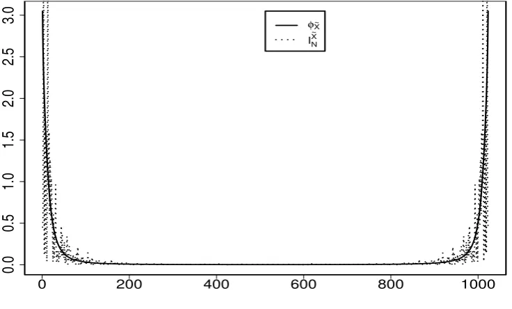
is illustrated in Figure 1. The periodogramIX˜
N and the spectral density φX˜ of the
Figures 1 and 2 near here
We then generate {Zt} from (10) with ∆ = 2501 . To consider all possible cases, the
proposed estimation procedure was applied to the LRD case of 0 < β < 12, the IRD case of −1
2 < β < 0 and the case of β = 0. Sample sizes of T = 512, 1024 and 2048
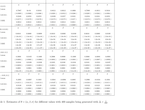
were considered. The number of 400 replications was used for each case. The function (16) is symmetrical respect toω, this reduce the number of computational operations in half. Simulation results are displayed in Tables 1 and 2 below. The results in Tables 1–2 show the empirical means, the empirical standard deviations and the empirical mean squared errors (MSEs) of the estimators. The empirical mean of the absolute value of the corresponding estimated bias is given in each bracket beneath the corresponding estimator. Each of the MSEs is computed as a sum of two terms: the square of the estimated bias and variance.
Tables 1–2 near here
The first section of Table 1 provides the corresponding results for the cases whereθ0 =
(0.8,0,0.5) and θ0 = (0.001,0,0.01). These results show that the estimation procedure
works well for the SRD case where the initial parameter value forβ is zero as well as for small σ0 and α0.
From the third section of Table 1 to Table 2, several different pairs of positive and negative β values are considered. The corresponding results show that the MSEs for both α0 and σ0 remain stable when β0 changes from a positive value to its negative
counterpart.
Individually, we have considered both relatively large and small values forβ to assess whether the estimation procedure is sensitive to the choice ofβ values. These results in Table 1 show that there is some MSE distortion in the case ofT = 512 for β0 when β0
is as small as either 0.01 or −0.01. WhenT increases to 1024 and then 2048, the MSEs become stable. For the case ofβ0 = 0.45 which appears in Table 3, the MSEs look quite
stable and very small.
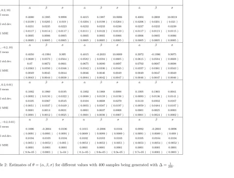
In Table 2, both relatively large and relatively small values for σ0 have been
consid-ered. For the case of σ0 = 10 in the first part of Table 2, the MSEs for the estimates of
all the components of θ0 are quite stable and very small particularly when T = 2048.
show that the MSEs become quite reasonable even when the sample size is as medium asT = 512. It is also observed from Table 2 that the change of the memory parameter value fromβ0 = 0.2 toβ0 =−0.2 does not affect the estimates ofα0 andσ0 significantly.
Tables 3–4 near here
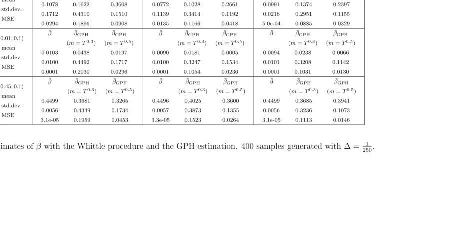
The memory parameter β is commonly estimated using the so–called GPH method proposed by Geweke and Porter–Hudak (1983) and then extended in Robinson (1995) and others. It has the property of being easily implemented and very fast. Deo and Hurvich (2001) study the bias and variance of this estimator for the memory parameter
β based on the fact that the periodogram of Z1, Z2, . . . , ZT is calculated for certain
Fourier frequenciesωj = 2πjT forj = 1,2, . . . , m, where m is chosen such that mT → ∞ as
m → ∞ and T → ∞. Discussion about the choice of m may be found from Robinson (1994).
Tables 3–4 compare the memory parameter estimators derived from the Whittle procedure with the GPH estimators form=T0.3 and m =T0.5. The motivation behind
the choice of m comes from Deo and Hurvich (2001) that study the GPH estimation method for m = T0.3, T0.4 and T0.5. The GPH estimation method is appropriate for
positive values of β which are those displayed in these tables. As in Deo and Hurvich (2001), the bias of the estimator ˜βGPHincreases when mincreases, however, the variance
decreases as m increases. In other words, the bias of the GPH estimator withm =T0.5
is greater than the bias with m =T0.3. However the MSE is smaller form =T0.5 than
that form=T0.3 due to smaller variance in each case. As expected, the MSE decreases
as the sample sizeT increases.
Tables 3–4 show that the Whittle procedure performs better than the GPH method in all the cases under consideration. Our experience also shows that the computing time for using the GPH method is much shorter than that for the Whittle method. It is our opinion that the GPH method may not be applicable to estimate all the parametersα,
β andσ involved in the model as the estimation method was proposed to estimate the β
parameter only. Our study however shows that the proposed estimation method based on the Whittle method is applicable to the estimation of all the parameters and works well numerically in all the cases under consideration.
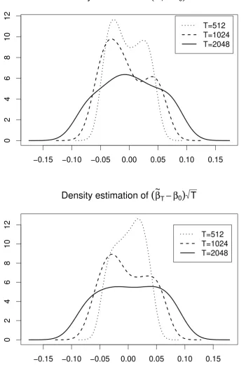
Regarding the asymptotic normality of the errors, Figures 3–4 show the density estimates of √T(˜θT −θ0) for T = 512,1024 and 2048. It is clear that as T increases
Figures 3–4 near here
In summary, the MSEs in Tables 1–4 demonstrate that both the proposed Whit-tle estimation procedure and the asymptotic convergence established in Theorem 2.1(i) work well numerically. Our preliminary simulation results further show that the MSEs become smaller when ∆ = 2501 . In addition, Figures 3–4 show graphically the asymp-totic normality of the errors established in Theorem 2.1(ii). In Section 4 below, both the proposed theory and the estimation procedure are also applied to several stock market indexes.
4. Applications to Market Indexes
Market indexes are a guideline of investor confidence and are inter–related to the performance of local and global economies. Investments on market indexes such as the Dow Jones, S&P 500, FTSE 100, etc. are common practice. In this section, we apply model (20) to model the stochastic volatility and then the estimation procedure to assess both the memory and volatility properties of such indexes. Section 4.1 provides the explicit expressions of both the mean and the variance functions of stochastic volatility process V(t). Section 4.2 describes briefly these indexes. Some empirical results are given in Section 4.3 below. Section 4.4 discusses a direct volatility estimation method.
4.1 Estimation of mean and variance
In addition to finding our estimates for the three parameters α, β and σ involved in model (20), we are also interested to estimate both the mean µV and the standard
deviationσV of the stochastic volatility process V(t).
Since we are concerned with the stationary version V(t) = eX(t) in model (20), we
are able to express both the mean and variance functions of V(t) as follows:
µV =µV(θ) = exp(σX2/2) and σ
2
V =σ
2
V(θ) =
exp(σ2
X)−1
exp(σ2
X), (23)
where
σX2 =σ
2
X(ϑ) =γX(0) =
σ2π
Γ2(1 +β)α1+2βcos(βπ). (24)
We then estimate the mean µV(θ) and the standard deviationσV(θ) by
˜
µV =µV(˜θT) and σ˜V =σV(˜θT) (25)
with ˜θT being defined before. For the market indexes, the corresponding estimates are
4.2 Data
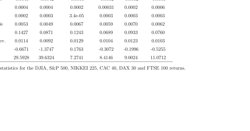
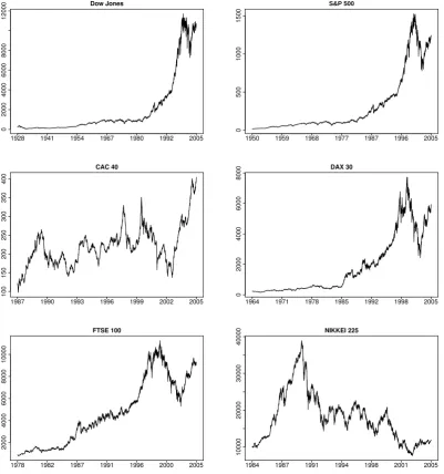
The data sets chosen for our empirical study are the following daily recorded financial stock indexes: a) two major American indexes: Dow Jones Industrial Average (from the 1st of October 1928 to the 29th of July 2005) and S&P 500 (from the 3rd of January 1950 to the 29th of July 2005); b) three of the major European indexes: CAC 40 (from the 30th of December 1987 to the 29th of July 2005), DAX 30 (from the 31st of December 1964 to the 29th of July 2005) and FTSE 100 (from the 31st of January 1978 to the 29th of July 2005); and c) the major Asian index, the NIKKEI 225 (from the 4th of January 1984 to the 29th of July 2005). A vast amount of information about market indexes is available on the Internet. Wikipedia and InvestorWords.com give easy access to informative glossaries of the stock market indexes. A figure of each of these indexes is given in Figure 5. The statistical summary of these financial series in Table 5 shows that the compounded returns series is stationary and has small standard deviation, small skewness and large kurtosis.
Figure 5 near here
Table 5 near here
4.3 Empirical Results
We have applied the proposed methodology to the real financial data. The results in Table 6 contain the estimates ofα, β,σ,µV, andσV. The values in brackets correspond
to the empirical MSEs showing that the asymptotic error is small in each case. The MSE values in Table 6 are indicative and calculated based on 400 replications with the sample size of T=2048. These values are expected to be smaller for larger sets of data.
Tables 6–7 near here
Results of Table 6 for the European indexes shows that the volatility of these indexes also displays LRD. The German DAX 30 has the largest mean and the largest standard deviation of the volatility process with values 1.3587 and 1.2499 respectively. In this respect, the CAC 40, the FTSE 100 and the S&P 500 have very similar values for the mean (1.1458, 1.1955 and 1.1550 respectively) and standard variation (0.6410, 0.7833 and 0.6676 respectively). This suggests that the volatility process of these two European indexes and the S&P 500 behave very similarly. In fact, the CAC 40 and FTSE 100 have a large percentage of shares belonging to foreign investors.
The long memory parameter estimate of the volatility process of the NIKKEI 225 has a value of 0.4860, again showing a very strong LRD. The mean (2.0768) and standard deviation (3.7801) of its volatility process are significatively larger than those of the European and American indexes. This is not surprising, since the risky behaviour of the Japanese stock market is a well–known fact.
Results of Table 7 compare the estimation of the β parameter using the Whittle method and the GPH method with m = T0.3, T0.4 and T0.5. The GPH estimator also
suggests that the volatility process of all the indexes displays some kind of LRD. Again, the choice ofm influences highly on the results.
4.4 Volatility Estimation
Estimatingα, β andσis equivalent to estimating the covariance matrix of{Xt}which
the information necessary to be able to obtain an estimate of the volatility process using the Kalman filter presented in Harvey (1989) and applied to this particular problem in Harvey (1998). The estimate ˜Xt is given by,
f
Xt = (I−σ2eC−1)Wt+σ2eC−1 ik, (26)
where C = 4CX +Ce with CX being the covariance matrix of {Xt} and Ce being the
diagonal matrix with values σ2
e, Iis the identity matrix and i is a vector of 1s and k is
estimated by the mean of Wt. Thus, Vet = exp(Xft). A comparison of this Vet with the
absolute value of the compounded returns can be found in Figure 6. The dotted line corresponds to |Wt| and the read line corresponds to the volatility process estimator.
The estimation has been done for the first 500 values of each of the indexes.
patterns that repeat at different scales of time. Therefore, investments based on the prediction of the volatility process of each of these stock market indexes may exploit this fact.
5. Discussion
This paper has established a general class of stochastic volatility models with either LRD, IRD, or SRD. An estimation procedure has been proposed to deal with cases where a class of non–Gaussian processes may display LRD, IRD or SRD. We then have conducted some comprehensive simulation studies to show that the proposed estimation procedure works well numerically not only for the LRD parameterβ, but also for both the drift parameter α and the volatility parameter σ. Our theory and estimation procedure has also been applied to estimate the volatility of some well–known stock market indexes. As imposed in Assumption 2.1(i), we have assumed the mutual independence of the two Brownian motion processes in order to clearly present the main ideas as well as the estimation procedure. As briefly discussed in Casas and Gao (2006), in order to take leverage effects into account we would need to impose some kind of dependent structure on the covariance matrix of the two Brownian motion processes. As expected, such dependent structure would make the current discussion much more complicated. We thus wish to leave such an extension for future research.
6. Acknowledgments
The authors would like to acknowledge constructive comments from Michael McAleer and two referees as well as the conference participants at the Perth International Con-ference on Time Series Econometrics, Finance and Risk in July 2006. The first author would also like to thank Helena Veiga for her comments. Financial support from the Australian Research Council is acknowledged.
Appendix A. Proof of Theorem 2.1
This appendix provides only an outline of the proof of Theorem 2.1, since some technical details are quite standard but tedious in this kind of proof and therefore omitted here.
Lemma A.1. Suppose that Assumptions 2.1 and 2.2 hold. Then for every continuous function w(ω, θ)
Z π
−πIT(ω)w(ω, θ) dω →
Z π
−πf(ω, θ0)w(ω, θ) dω (27)
with probability one as T → ∞.
Proof: The conclusion in (27) is the same as Lemma 1 of Fox and Taqqu (1986) for the cases where the process involved is Gaussian. The proof of their Lemma 1 basically follows that of Lemma 1 of Hannan (1973), which does not impose any Gaussian assumptions on the process involved.
In view of the expression ofZt=µ+ 2Xt+et in (10) as well as Lemma 1 of Hannan
(1973), therefore the proof of Lemma 1 of Fox and Taqqu (1986) remains valid for the case where{Xt} is the Gaussian time series with LRD, {et} is a sequence i.i.d. random
errors and thus {Zt} is non–Gaussian. This is mainly because of the following two
reasons.
The first reason is that Assumption 2.1(ii) guarantees that {Xt}admits a backward
expansion of the form (see Fox and Taqqu 1986, p.520)
Xt= ∞
X
s=0
bsut−s, (28)
where {bs} is a sequence of suitable real numbers such that {Xt} is a Gaussian process
with its spectral density function being given by fX(ω, θ), and {us : −∞ < s < ∞} is
a sequence of independent and normally distributed random variables with E[us] = 0
and E[u2
s] = 1. Thus, {Zt} can be written into a partial sum of independent random
variables of the form
Zt=µ+et+ 2 ∞
X
s=0
bsut−s. (29)
The second reason is that Lemma 1 of Hannan (1973) is applicable to non–Gaussian time series and thus to {Zt} of the form (29).
Lemma A.2. Suppose that Assumptions 2.1 and 2.2 hold. Then as T → ∞
WT(θ)→W(θ) =
1 4π
Z π
−π
(
log(f(ω, θ)) + f(ω, θ0)
f(ω, θ)
)
dω. (30)
Proof: The proof of (30) follows from (27).
Lemma A.3. Suppose that Assumptions 2.1 and 2.2 hold. Then as T → ∞
˜
Proof: Lemma A.2 implies that the following holds with probability one forθ 6=θ0,
WT(θ)−WT(θ0)→K(θ, θ0) =
1 4π
Z π
−π
(
f(ω, θ0)
f(ω, θ) −1−log
f(ω, θ0)
f(ω, θ)
!)
dω >0 (32)
asT → ∞.
Thus, for any given ǫ >0
lim inf
T→∞||θ−θinf0||≥ǫ
(WT(θ)−WT(θ0))>0 (33)
with probability one. The proof of ˜θT →θ˜0with probability one follows from Assumption
2.1(iii). Thus, the proof of Lemma A.3 is finished.
Proof of Theorem 2.1(i): The first part of Theorem 2.1 has already been proved in Lemma A.3.
Proof of Theorem 2.1(ii): The proof of the second part of Theorem 2.1 is a direct application of Theorem 1(ii) of Heyde and Gay (1993). Note that Assumption 2.1 implies that Condition (A1) of Heyde and Gay (1993) is satisfied because of (28) and the expression ofZt=µ+ 4Xt+et. Assumption 2.2 implies that conditions (A2) and (A3)
of Heyde and Gay (1993) are satisfied forfX(ω, θ) and then fZ(ω, θ). Thus, by applying
the Mean–Value Theorem and Theorem 1(ii) of Heyde and Gay (1993), the proof of the asymptotic normality is completed.
Using Assumption 2.2(viii) and Theorem 2.1(i), the proof of Σ(˜θT)→ Σ(θ0) follows
asT → ∞.
References
Andersen, T. G., and Lund, J.(1997), “Estimating Continuous–Time Stochastic Volatility Models
of the Short Term Interest Rate”,Journal of Econometrics, 77, 343–378.
Andersen, T. G., and Sørensen, B. E.(1996), “GMM Estimation of a Stochastic Volatility Model:
A Monte Carlo Study”,Journal of Business and Economic Statistics, 14, 328–352.
Andrews, D. W. K., and Sun, Y.(2004), “Adaptive Local Polynomial Whittle Estimation of Long–
Range Dependence”,Econometrica, 72, 569–614.
Anh, V., and Heyde, C. (ed.) (1999), “Special Issue on Long-Range Dependence”,Journal of
Sta-tistical Planning & Inference, 80, 1.
Anh, V., Heyde, C., and Leonenko, N.(2002), “Dynamic Models of Long Memory Processes Driven
by L´evy Noise”,Journal of Applied Probability, 39, 730–747.
Anh, V., and Inoue, A. (2005), “Financial Markets with Memory I: Dynamic Models”, Stochastic
Analysis & Its Applications, 23, 275–300.
Processes and Expected Utility Maximization”,Stochastic Analysis & Its Applications, 23, 301–328.
Anh, V., Leonenko, N. N., Sakhno, L. M.(2004). “On a Class of Minimum Contrast Estimators
for Fractional Stochastic Processes and Fields”,Journal of Statistical Planning and Inference, 123, 161– 185.
Arapis, M., and Gao, J.(2006), “Empirical Comparisons in Short–Term Interest Rate Models using
Nonparametric Methods”,Journal of Financial Econometrics, 4, 310–345.
Asai, M., McAleer, M., and Yu, J.(2006), “Multivariate Stochastic Volatility: a review”,
Econo-metric Reviews, 25, 145–175.
Baillie, R., and King, M. L. (ed.) (1996), “Special Issue of Journal of Econometrics”, Annals of
Econometrics, 73, 1.
Barndorff–Nielsen, O. E., and Leonenko, N. N.(2005). “Spectral Properties of Superpositions
of Ornstein–Uhlenbeck Type Processes”,Methodology and Computing in Applied Probability, 7, 335–352.
Beran, J.(1994),Statistics for Long–Memory Processes, New York: Chapman and Hall.
Black, F., and Scholes, M.(1973), “The Pricing of Options and Corporate Liabilities”,Journal of
Political Economy, 3, 637–654.
Breidt, F. J., Crato, N., and de Lima, P. J. F.(1998), “The Detection and Estimation of Long–
Memory in Stochastic Volatility”,Journal of Econometrics, 83, 325–348.
Brockwell, P., and Davis, R.(1990),Time Series: Theory and Methods, New York: Springer.
Casas, I., and Gao, J.(2006), “Econometric Estimation in Stochastic Volatility Models with Long–
Range Dependence,” Working paper available at http://www.maths.uwa.edu.au/˜jiti/casgaolrd.pdf.
Comte, F.(1996), “Simulation and Estimation of Long Memory Continuous Time Models”, Journal
of Time Series Analysis, 17, 19–36.
Comte, F., and Renault, E.(1996), “Long Memory Continuous–Time Models”,Journal of
Econo-metrics, 73, 101–150.
Comte, F., and Renault, E.(1998), “Long Memory in Continuous–Time Stochastic Volatility
Mod-els”,Mathematical Finance, 8, 291–323.
Cox, J. C., Ingersoll, J.E. and Ross, S.A. (1985), “A Theory of the Term Structure of Interest
Rates,”Econometrica, 53, 385–407.
Deo, R., and Hurvich, C. M.(2001), “On the Log–Periodogram Regression Estimator of the
Mem-ory Parameter in Long MemMem-ory Stochastic Volatility Models”,Econometric Theory, 17, 686–710.
Ding, Z., Granger, C. W. J., and Engle, R.(1993), “A Long Memory Property of Stock Market
Returns and a New Model,”Journal of Empirical Finance, 1, 83–105.
Fan, J., and Zhang, C. M.(2003), “A Re-examination of Stanton’s Diffusion Estimators with
Appli-cations to Financial Model Validation.”Journal of the American Statistical Association, 461, 118–134.
Fox, R., and Taquu, M.S. (1986), “Large–Sample Properties of Parameter Estimates for Strongly
Dependent Stationary Gaussian Time Series”,Annals of Statistics, 14, 512–532.
Gao, J.(2004), “Modelling Long–Range Dependent Gaussian Processes with Application in Continuous–
Time Financial Models”,Journal of Applied Probability, 41, 467–482.
Gao, J., Anh, V., and Heyde, C. (2002), “Statistical Estimation of Nonstationary Gaussian
Pro-cesses with Long–Range Dependence and Intermittency”, Stochastic Processes & Their Applications, 99, 295–321.
with Long–Range Dependence and Intermittency”,Journal of Time Series Analysis, 22, 517–535.
Geweke, J., and Porter–Hudak, S. (1983), “The Estimation and Application of Long Memory
Time Series Models”,Journal of Time Series Analysis, 4, 221–238.
Hannan, E. J.(1973), “The Asymptotic Theory of Linear Time–Series Models”, Journal of Applied
Probability, 10, 130–145.
Harvey, A. C.(1989),Forecasting, Structural Time Series Models and the Kalman Filter, New York:
Cambridge University Press.
Harvey, A. C.(1998), “Long Memory in Stochastic Volatility”, inKnight, J. and Satchell, S. ,
Forecasting Volatility in the Financial Markets, Oxford: Butterworth and Heinemann.
Heyde, C., and Gay, R.(1993), “Smoothed Periodogram Asymptotics and Estimation for Processes
and Fields with Possible Long–Range Dependence”, Stochastic Processes and Their Applications, 45, 169–182.
Hosoya, Y.(1997), “A Limit Theory for Long–Range Dependence and Statistical Inference on Related
Models”,Annals of Statistics, 25, 105–137.
Hull, J., and White, A. (1987), “The Pricing of Options on Assets with Stochastic Volatilities”,
Journal of Finance, 2, 281–300.
Leonenko, N. N. and Sakhno, L. M. (2006). “On the Whittle Estimators for Some Classes of
Continuous Parameter Random Processes and Fields”,Statistics and Probability Letters, 76, 781–795.
Priestley, M. B.(1981),Spectral Analysis and Time Series, New York: Academic Press.
Robinson, P.(1994), “Rates of Convergence and Optimal Spectral Bandwidth for Long Range
Depen-dence”,Probability Theory and Related Fields, 99, 443–473.
Robinson, P.(1995), “Gaussian Semiparametric Estimation of Long–Range Dependence”,Annals of
Statistics, 23, 1630–1661.
Robinson, P. M.(ed.) (2003), “Time Series with Long Memory”, Advanced Texts in Econometrics,
Oxford: Oxford University Press.
Stoyanov, J.(2004), “Stieltjes Classes for Moment-Indeterminate Probability Distributions”,Journal
of Applied Probability, 41A, 281–294.
Sun, Y., and Phillips, P. C. B.(2003), “Nonlinear Log–periodogram Regression for Perturbed
Frac-tional Processes”,Journal of Econometrics, 115, 355–389.
Taylor, S. J.(1986),Modelling Financial Time Series, Chichester. U.K.: John Wiley.
Taylor, S. J. (1994), “Modelling Stochastic Volatility: A Review and Comparative Study”,
Mathe-matical Finance, 4, 183–204.
Vasicek, O.(1977), “An Equilibrium Characterization of the Term Structure”, Journal of Financial
Economics, 5, 177–188.
Whittle, P.(1951),Hypothesis Testing in Time Series Analysis, New York: Hafner.
Appendix B. Tables and Figures
0 200 400 600 800 1000
−2
−1
0
1
[image:22.595.122.491.113.334.2]2
Figure 1: Sample path for data generated with θ0 = (0.1,0.1,0.1) and ∆ = 1.
0 200 400 600 800 1000
0.0
0.5
1.0
1.5
2.0
2.5
3.0 φX~
I N X ~
[image:22.595.123.491.415.637.2]T = 512 T = 1024 T = 2048
θ0= (0.8,0,0.5)
Empirical mean
Empirical std.dev.
Empirical MSE
¯
α β¯ σ¯
0.7987 9e-04 0.5010
( 0.0303 ) ( 0.0308 ) ( 0.0306 )
0.0348 0.0352 0.0353
( 0.0171 ) ( 0.0170 ) ( 0.0176 )
0.0012 0.0012 0.0012
( 0.0011 ) ( 0.0012 ) ( 0.0012 )
¯
α β¯ σ¯
0.8012 0.0012 0.4960
( 0.0291 ) ( 0.0312 ) ( 0.0286 )
0.0339 0.0357 0.0331
( 0.0173 ) ( 0.0173 ) ( 0.017 )
0.0012 0.0013 0.0011
( 0.0011 ) ( 0.0012 ) ( 0.0009 )
¯
α β¯ ¯σ
0.7989 -0.0011 0.5010
( 0.0285 ) ( 0.0282 ) ( 0.0304 )
0.0334 0.0331 0.0352
( 0.0174 ) ( 0.0173 ) ( 0.0178 )
0.0011 0.0011 0.0012
( 0.0011 ) ( 0.0010 ) ( 0.0012 )
θ0= (0.001,0,0.01)
Empirical mean
Empirical std.dev.
Empirical MSE
¯
α β¯ ¯σ
0.0010 0.0000 0.0099
( 1.0e-04 ) ( 1.0e-04 ) ( 5.0e-04 )
1.0e-04 1.0e-04 6.0e-04
( 1.0e-04 ) ( 1.0e-04 ) ( 5.0e-04 )
1.0e-08 1.0e-08 3.7e-07
( 2.0e-08 ) ( 2.0e-08 ) ( 4.1e-07 )
¯
α β¯ σ¯
0.0010 0.0000 0.0100
( 1.0e-04 ) ( 1.0e-04 ) ( 3.0e-04 )
1.0e-04 1.0e-04 5.0e-04
( 1.0e-04 ) ( 1.0e-04 ) ( 3.0e-04 )
1.0e-08 1.0e-08 2.5e-07
( 2.0e-08 ) ( 2.0e-08 ) ( 1.8e-07 )
¯
α β¯ σ¯
0.0010 0.0000 0.0100
( 1.0e-04 ) ( 1.0e-04 ) ( 2.0e-04 )
1.0e-04 1.0e-04 3.0e-04
( 1.0e-04 ) ( 1.0e-04 ) ( 3.0e-04 )
1.0e-08 1.0e-08 9.0e-08
( 2.0e-08 ) ( 2.0e-08 ) ( 1.3e-07 )
θ0= (0.3,0.01,0.1)
Empirical mean
Empirical std.dev.
Empirical MSE
¯
α β¯ ¯σ
0.3008 0.0103 0.1000
( 0.0092 ) ( 0.0085 ) ( 0.0096 )
0.0104 0.0100 0.0109
( 0.0050 ) ( 0.0053 ) ( 0.0052 )
0.0001 0.0001 0.0001
( 9.6e-05 ) ( 9.5e-05 ) ( 0.0001 )
¯
α β¯ σ¯
0.2996 0.0090 0.1009
( 0.0092 ) ( 0.0086 ) ( 0.0091 )
0.0105 0.0100 0.0104
( 0.0051 ) ( 0.0053 ) ( 0.0051 )
0.0001 0.0001 0.0001
( 0.0001 ) ( 8.6e-05 ) ( 9.3e-05 )
¯
α β¯ σ¯
0.3006 0.0094 0.0995
( 0.0087 ) ( 0.0087 ) ( 0.0092 )
0.0101 0.0101 0.0107
( 0.0052 ) ( 0.0051 ) ( 0.0053 )
0.0001 0.0001 0.0001
( 9.3e-05 ) ( 9.2e-05 ) ( 0.0001 )
θ0= (0.3,−0.01,0.1)
Empirical mean
Empirical std.dev.
Empirical MSE
¯
α β¯ σ¯
0.2995 -0.0097 0.1003
( 0.0111 ) ( 0.0113 ) ( 0.0112 )
0.0128 0.0129 0.0129
( 0.0063 ) ( 0.0062 ) ( 0.0065 )
0.0002 0.0002 0.0002
( 0.0001 ) ( 0.0002 ) ( 0.0002 )
¯
α β¯ σ¯
0.3004 -0.0096 0.0985
( 0.0107 ) ( 0.0114 ) ( 0.0105 )
0.0124 0.0131 0.0121
( 0.0063 ) ( 0.0063 ) ( 0.0062 )
0.0002 0.0002 0.0001
( 0.0001 ) ( 0.0001 ) ( 0.0001 )
¯
α β¯ ¯σ
0.2996 -0.0104 0.1004
( 0.0104 ) ( 0.0103 ) ( 0.0111 )
0.0122 0.0121 0.0129
( 0.0064 ) ( 0.0063 ) ( 0.0065 )
0.0001 0.0001 0.0002
( 0.0001 ) ( 0.0001 ) ( 0.0001 )
[image:23.595.110.699.54.530.2]T = 512 T = 1024 T= 2048
θ0= (0.4,0.2,10)
Empirical mean
Empirical std.dev.
Empirical MSE
¯
α β¯ ¯σ
0.4000 0.1995 9.9998
( 0.0199 ) ( 0.0205 ) ( 0.019 )
0.0231 0.0235 0.0223
( 0.0117 ) ( 0.0114 ) ( 0.0117 )
0.0005 0.0006 0.0005
( 0.0005 ) ( 0.0005 ) ( 0.0005 )
¯
α β¯ σ¯
0.4015 0.1987 10.0006
( 0.0204 ) ( 0.0198 ) ( 0.0204 )
0.0232 0.0233 0.0236
( 0.0111 ) ( 0.0122 ) ( 0.0119 )
0.0005 0.0005 0.0006
( 0.0005 ) ( 0.0005 ) ( 0.0005 )
¯
α β¯ σ¯
0.4004 0.2008 10.0019
( 0.0206 ) ( 0.0201 ) ( 0.021 )
0.0237 0.0232 0.0239
( 0.0117 ) ( 0.0115 ) ( 0.0115 )
0.0006 0.0005 0.0006
( 0.0005 ) ( 0.0005 ) ( 0.0005 )
θ0= (0.4,−0.2,10)
Empirical mean
Empirical std.dev.
Empirical MSE
¯
α β¯ ¯σ
0.4050 -0.1994 9.995
( 0.0600 ) ( 0.0573 ) ( 0.0564 )
0.07 0.0672 0.0661
( 0.0363 ) ( 0.0350 ) ( 0.0346 )
0.0049 0.0045 0.0044
( 0.0043 ) ( 0.0044 ) ( 0.0038 )
¯
α β¯ σ¯
0.4015 -0.2033 10.0009
( 0.0582 ) ( 0.0594 ) ( 0.0605 )
0.0675 0.0680 0.0697
( 0.0342 ) ( 0.0330 ) ( 0.0345 )
0.0046 0.0046 0.0049
( 0.0044 ) ( 0.0042 ) ( 0.0047 )
¯
α β¯ σ¯
0.3972 -0.1996 9.9975
( 0.0615 ) ( 0.0584 ) ( 0.0608 )
0.0702 0.0687 0.0698
( 0.0337 ) ( 0.0361 ) ( 0.0343 )
0.0049 0.0047 0.0049
( 0.0046 ) ( 0.0047 ) ( 0.0046 )
θ0= (0.1,0.2,0.01)
Empirical mean
Empirical std.dev.
Empirical MSE
¯
α β¯ ¯σ
0.1002 0.1960 0.0195
( 0.0092 ) ( 0.0150 ) ( 0.0322 )
0.0105 0.0367 0.0545
( 0.0051 ) ( 0.0337 ) ( 0.0449 )
0.0001 0.0014 0.0031
( 0.0001 ) ( 0.0012 ) ( 0.0025 )
¯
α β¯ σ¯
0.1002 0.1968 0.0088
( 0.0088 ) ( 0.0159 ) ( 0.0198 )
0.0104 0.0608 0.0279
( 0.0055 ) ( 0.0587 ) ( 0.0197 )
0.0001 0.0037 0.0008
( 0.0001 ) ( 0.0036 ) ( 0.0007 )
¯
α β¯ σ¯
0.1005 0.1965 0.0041
( 0.0093 ) ( 0.0136 ) ( 0.0141 )
0.0110 0.0502 0.0167
( 0.0059 ) ( 0.0484 ) ( 0.0107 )
0.0001 0.0025 0.0003
( 0.0001 ) ( 0.0024 ) ( 0.0002 )
θ0= (0.1,−0.2,0.01)
Empirical mean
Empirical std.dev.
Empirical MSE
¯
α β¯ ¯σ
0.1006 -0.2004 0.0106
( 0.0091 ) ( 0.0091 ) ( 0.0091 )
0.0104 0.0105 0.0104
( 0.0051 ) ( 0.0052 ) ( 0.005 )
0.0001 0.0001 0.0001
( 9.8e-05 ) ( 0.0001 ) ( 1e-04 )
¯
α β¯ σ¯
0.1015 -0.2006 0.0104
( 0.0089 ) ( 0.0089 ) ( 0.0089 )
0.0102 0.0103 0.0103
( 0.0053 ) ( 0.0052 ) ( 0.0051 )
0.0001 0.0001 0.0001
( 8.1e-05 ) ( 9.6e-05 ) ( 9.9e-05 )
¯
α β¯ σ¯
0.0992 -0.2003 0.0096
( 0.0091 ) ( 0.0089 ) ( 0.009 )
0.0105 0.0104 0.0104
( 0.0053 ) ( 0.0054 ) ( 0.0052 )
0.0001 0.0001 0.0001
( 9.7e-05 ) ( 0.0001 ) ( 0.0001 )
[image:24.595.113.694.54.531.2]T = 512 T = 1024 T = 2048
θ0= (0.1,0.1,0.1)
Empirical mean
Empirical std.dev. Empirical MSE
¯
β β¯GPH β¯GPH
(m=T0.3) (m=T0.5)
0.1078 0.1622 0.3608
0.1712 0.4310 0.1510
0.0294 0.1896 0.0908
¯
β β¯GPH β¯GPH
(m=T0.3) (m=T0.5)
0.0772 0.1028 0.2661
0.1139 0.3414 0.1192
0.0135 0.1166 0.0418
¯
β β¯GPH β¯GPH
(m=T0.3) (m=T0.5)
0.0991 0.1374 0.2397
0.0218 0.2951 0.1155
5.0e-04 0.0885 0.0329
θ0= (0.3,0.01,0.1)
Empirical mean
Empirical std.dev. Empirical MSE
¯
β β¯GPH β¯GPH
(m=T0.3) (m=T0.5)
0.0103 0.0438 0.0197
0.0100 0.4492 0.1717
0.0001 0.2030 0.0296
¯
β β¯GPH β¯GPH
(m=T0.3) (m=T0.5)
0.0090 0.0181 0.0005
0.0100 0.3247 0.1534
0.0001 0.1054 0.0236
¯
β β¯GPH β¯GPH
(m=T0.3) (m=T0.5)
0.0094 0.0238 0.0066
0.0101 0.3208 0.1142
0.0001 0.1031 0.0130
θ0= (0.5,0.45,0.1)
Empirical mean
Empirical std.dev. Empirical MSE
¯
β β¯GPH β¯GPH
(m=T0.3) (m=T0.5)
0.4499 0.3681 0.3265
0.0056 0.4349 0.1734
3.1e-05 0.1959 0.0453
¯
β β¯GPH β¯GPH
(m=T0.3) (m=T0.5)
0.4496 0.4025 0.3600
0.0057 0.3873 0.1355
3.3e-05 0.1523 0.0264
¯
β β¯GPH β¯GPH
(m=T0.3) (m=T0.5)
0.4499 0.3685 0.3941
0.0056 0.3236 0.1073
[image:25.595.120.688.166.413.2]3.1e-05 0.1113 0.0146
Table 3: Estimates of β with the Whittle procedure and the GPH estimation. 400 samples generated with ∆ = 2501 .
T= 512 T = 1024 T= 2048
θ0= (0.4,0.2,10)
Empirical mean
Empirical std.dev. Empirical MSE
¯
β β¯GPH β¯GPH
(m=T0.3) (m=T0.5)
0.1995 0.2480 0.2362
0.0235 0.4944 0.1597
0.0006 0.2468 0.0268
¯
β β¯GPH β¯GPH
(m=T0.3) (m=T0.5)
0.1987 0.1673 0.2219
0.0233 0.3295 0.1416
0.0005 0.1096 0.0205
¯
β β¯GPH β¯GPH
(m=T0.3) (m=T0.5)
0.2008 0.2282 0.22801
0.0232 0.3231 0.1093
0.0005 0.1052 0.0127
θ0= (0.1,0.2,0.01)
Empirical mean
Empirical std.dev. Empirical MSE
¯
β β¯GPH β¯GPH
(m=T0.3) (m=T0.5)
0.1960 0.0546 0.0387
0.0367 0.4103 0.1657
0.0014 0.1895 0.0535
¯
β β¯GPH β¯GPH
(m=T0.3) (m=T0.5)
0.1968 0.0482 0.0689
0.0608 0.3397 0.1437
0.0037 0.1384 0.0378
¯
β β¯GPH β¯GPH
(m=T0.3) (m=T0.5)
0.1965 0.0167 0.0476
0.0502 0.3268 0.1227
0.0025 0.1404 0.0383
θ0= (1,0.2,0.01)
Empirical mean
Empirical std.dev. Empirical MSE
¯
β β¯GPH β¯GPH
(m=T0.3) (m=T0.5)
0.1999 0.0612 0.0085
0.0220 0.4126 0.1632
0.0005 0.1895 0.0633
¯
β β¯GPH β¯GPH
(m=T0.3) (m=T0.5)
0.1991 -0.0130 -0.0132
0.0222 0.3107 0.1234
0.0005 0.1419 0.0607
¯
β β¯GPH β¯GPH
(m=T0.3) (m=T0.5)
0.1918 -0.0343 -0.0042
0.0463 0.3135 0.0991
[image:26.595.122.684.166.414.2]0.0022 0.1532 0.0515
Table 4: Estimates of β with the Whittle procedure and the GPH estimation. 400 samples generated with ∆ = 2501 .
DJIA S&P 500 NIKKEI 225 CAC 40 DAX 30 FTSE 100
T 19289 11976 5308 4587 10586 5387
Minimum -0.2563 -0.2290 -0.0721 -0.0951 -0.1306 -0.1303
1st Quantile -0.0046 -0.0042 -0.0066 -0.0052 -0.0062 -0.0053
Median 0.0004 0.0004 0.0002 0.00031 0.0002 0.0006
Mean 0.0002 0.0003 3.4e-05 0.0003 0.0003 0.0003
3rd Quantile 0.0053 0.0049 0.0067 0.0059 0.0070 0.0062
Maximum 0.1427 0.0871 0.1243 0.0689 0.0933 0.0760
Standard dev. 0.0114 0.0092 0.0129 0.0104 0.0123 0.0103
Skewness -0.6671 -1.3747 0.1763 -0.3072 -0.1996 -0.5255
[image:27.595.159.651.183.411.2]Kurtosis 29.5928 39.6324 7.2741 8.4146 9.0024 11.0712
Table 5: Summary statistics for the DJIA, S&P 500, NIKKEI 225, CAC 40, DAX 30 and FTSE 100 returns.
Index α¯ β¯ σ¯ µ¯V σ¯V
DJIA 0.0478 0.4783 0.0055 1.3482 1.2191
(2.7e-05) (3.1e-0.5) (1.7e-05)
S&P 500 0.0732 0.4563 0.0086 1.1550 0.6676
(3.3e-05) (3.6e-05) (2.0e-05)
CAC 40 0.2122 0.4549 0.0237 1.1458 0.6410
(0.0004) (0.0005) (0.0002)
DAX 30 0.0877 0.4841 0.0085 1.3587 1.2499
(9.8e-05) (0.0001) (5.5e-05)
FTSE 100 0.0588 0.4608 0.0073 1.1955 0.7833
( 2.4e-05) (2.7e-05) (1.9e-05)
NIKKEI 225 0.0830 0.4860 0.0115 2.0768 3.7801
[image:28.595.136.484.143.415.2](7.1e-05) (7.9e-05) (5.2e-05)
Table 6: Estimates of market indexes volatility parameters when independence between the two Brownian motions is assumed. The empirical MSE of the estimators is displayed in brackets.
Index β¯GPH(m =n0.3) β¯GPH(m=n0.4) β¯GP H(m =n0.5) β¯
DJIA 0.5772 0.7033 0.5496 0.4783
S&P 500 0.4892 0.5554 0.4929 0.4563
CAC 40 0.3456 0.2319 0.3257 0.4549
DAX 30 0.6505 0.6300 0.3620 0.4841
FTSE 100 0.4805 0.5034 0.5462 0.4608
[image:28.595.115.507.545.693.2]NIKKEI 225 0.4522 0.4817 0.3929 0.4860
−0.15 −0.10 −0.05 0.00 0.05 0.10 0.15
0
2
4
6
8
10
12
Density estimation of
(
α
~
T− α0
)
T
T=512 T=1024 T=2048
−0.15 −0.10 −0.05 0.00 0.05 0.10 0.15
0
2
4
6
8
10
12
Density estimation of
(
β
~
T− β0
)
T
T=512 T=1024 T=2048
Figure 3: Density function estimates of √T(¯αT − α0) and
√
T( ¯βT − β0) for θ0 =
[image:29.595.132.484.170.704.2]−0.15 −0.10 −0.05 0.00 0.05 0.10 0.15
0
2
4
6
8
10
12
Density estimation of
(
σ
~
T− σ0
)
T
[image:30.595.137.477.336.559.2]T=512 T=1024 T=2048
0
2000
4000
6000
8000
12000
Dow Jones
Index
1928 1941 1954 1967 1980 1992 2005
0
500
1000
1500
S&P 500
1950 1959 1968 1977 1987 1996 2005
100
150
200
250
300
350
400
CAC 40
Index
1987 1990 1993 1996 1999 2002 2005
0
2000
4000
6000
8000
DAX 30
Index
1964 1971 1978 1985 1992 1998 2005
2000
4000
6000
8000
10000
FTSE 100
Index
1978 1982 1987 1991 1996 2000 2005
10000
20000
30000
40000
NIKKEI 225
Index
[image:31.595.109.511.212.641.2]1984 1987 1991 1994 1998 2001 2005
0 100 200 300 400 500
0
10
20
30
DJIA
Wt V ~ t
0 100 200 300 400 500
0
2
4
6
8
10
S&P 500
Wt V~t
0 100 200 300 400 500
0
5
10
15
CAC 40
Wt V ~ t
0 100 200 300 400 500
0
2
4
6
8
DAX 30
Wt V~t
0 100 200 300 400 500
0
2
4
6
8
FTSE 100
Wt V ~ t
0 100 200 300 400 500
0
2
4
6
8
NIKKEI 225
[image:32.595.113.509.189.615.2]Wt V~t