Performance Analysis of Adaptive Channel
Equalizer using Population based Update
Algorithms
H. Pal Thethi
Swati Swayamsiddha
School of Electronics Engineering School of Electronics Engineering KIIT University, Bhubaneswar, India KIIT University, Bhubaneswar, India
ABSTRACT
Digital channel is modeled as a low pass filter; thereby the data transmitted through this band limited channel suffers from distortions. Adaptive Channel equalization involves compensation for an unknown time-varying channel which is achieved with the help of an adaptive algorithm. This update algorithm is primarily used to update the equalizer coefficients. In the present work channel equalization is formulated as an optimization problem and minimization of squared error, which serves as objective function, is achieved iteratively using two population based algorithms namely Bacterial foraging optimization (BFO) and Differential Evolution (DE) and its different variants. Finally, these approaches are compared with respect to MSE convergence and bit error rate.
Keywords
Adaptive Channel Equalization, Bacterial Foraging Optimization, Differential Evolution
1.
INTRODUCTION
Adaptive channel equalization plays a vital role in digital communication technology as it mitigates the effect of distortion in received signals, which are introduced as a result of inter-symbol interference (ISI) [1]. Basically an equalizer is an inverse filter whose transfer function is inverse to that of the channel. The adaptive equalization is an optimization problem, where the objective is to iteratively reduce the mean square error (MSE) between the output of equalizer and delayed signal from the source using an update algorithm [2]. The gradient algorithm based adaptive channel equalization has been reported in [3] and [4] which suffer from local optimization of the MSE. Artificial neural networks and Multilayer Perceptron based channel equalizers are proposed in [5], [6] which do not perform satisfactorily for nonlinear channel equalization. The inconvenience of these algorithms is its slow convergence and they can at times produce unpredictable solutions during the training phase. Literature survey reveals that recently a lot of work has been done using the derivative-free algorithms [7], [8] for nonlinear channel equalization using population based heuristic methods.
The present work investigates the performance of two recently proposed population based derivative free algorithms for adaptive channel equalization namely Bacterial foraging optimization (BFO) and Differential evolution (DE) [12], [13]. Further in the present work, different types of DEs are used in updating the parameters of equalizer and its performance in terms of convergence graph with mean square error (MSE) as
objective function and bit error rate vs. SNR plot is compared with Bacteria foraging optimization (BFO) based learning algorithm. The entire paper is organized as follows. In section 2, basic model of channel equalization is described. Section 3 briefly introduces both the population based algorithms used. The experimental results in terms of convergence performance and BER performance for both the algorithms have been presented in section 4 and the paper is concluded in section 5 and the relevant references are given in section 6.
2.
THE
CHANNEL
EQUALIZATION MODEL
The basic equalization process is illustrated in Fig.1, where x(k) is the input symbol sequence at instance k. To mimic the actual channel nonlinear block is added the output of which is y(k). Channel noise represents Additive White Gaussian Noise (AWGN). z(k) is the output of the equalizer and d(k) is the delayed version of the transmitted data. The output of the adaptive filter is subtracted from a desired response signal to calculate the error signal, which is mathematically given as e(k)=z(k)-d(k). The mean square error (MSE) is calculated from this error signal. The objective of an equalizer is iterative minimization of the MSE using the adaptive algorithms such that the equalizer produces an exact replica of the transmitted signal.x(k)
noise +
z(k) d(k
)
-
+ [image:1.595.297.527.531.643.2]
y(k) e(k)
Fig 1: Digital Communication system Equalizer
Update algorithm
Delay
Σ
Σ
3.
UPDATE ALGORITHMS
A).
BFO based channel equalization
This algorithm tries to mimick the food gathering behaviour of e-coli bacterium as an optimization problem which is then used to update the parameters of equalizer [12]. In its entire lifecycle an e-coli bacteria does two activities only, it runs or it tumbles. This algorithm involves four basic operators like chemotaxis, reproduction,elimination and dispersal.
Step 1: Initialization of parameters
n= number of bacteria used in searching space,
N=number of input samples, p= parameters to be optimized, Ns= run length after which bacteria tumbles in the chemotaxis loop, Nc=number of iterations used in chemotactic loop, generally Nc>Ns , Nre= maximum number of reproduction loop, Ped=probability of elimination and dispersal, the location of each bacterium
P(1-p,1-n,1) is specified by random binary number between [0,1], C(i)=value of run/swim length, which is constant for each bacterium used in search space.
Step 2: Generation of input signal
i). Random binary input signal between [-1,1] are generated and feed to channel. The output of channel is contaminated with noise of known strength to generate the input signal.
ii).Same random binary input is delayed to approximately half the order of equalizer, which is used to obtain the desired signal.
Step -3 Algorithm used for optimization
Here the bacterial population and other operators involved in the algorithm like chemotaxis (j), reproduction (k), elimination and dispersal (l) are modeled mathematically. Initially to start with
0
k
l
j
.(i) Update elimination dispersal loop
(ii) Update reproduction loop
(iii) Update chemotaxis loop
(a) The fitness value for each ithbacterium, for
i
1
,
2
,...
...,
n
is iteratively computed as follows:(1) Nnumbers of binary input signals are passed through the equalizer structure.
(2) The output of equalizer is then compared with the corresponding desired signal, d(k) to calculate the error
e(k). The error e(k) at kth input sample is computed. (3)The sum of squared error is averaged over entire number of input signals “N” and it is registered in
.
(4)For Loop ends.
(b)The tumbling/swimming operation is performed for
n
i
1
,
2
,...
...,
Tumble: A random vector
(
i
)
with each element, as a random number between [-1, 1] is generated.The new position of ith bacterium after a tumble is
calculated by using following equation.
)
(
)
(
)
,
,
(
)
,
,
1
(
j
k
l
p
j
k
l
C
i
i
p
i
i
(1) where
)
(
)
(
)
(
)
(
i
i
i
i
T
(2)Equation (1) is used to calculate the cost function (MSE) .
Swim – (i) Initially counter for swim length is assumed to be 0.
(ii) While
c
L
UpdateIf , the position of ith bacterium
)
,
,
1
(
j
k
l
P
i
is updated according to (1). This new position is now used to compute the new cost function.ELSE when
c
N
s: end of the WHILE statement.(c) This is repeated for next bacterium if
i
n
.
(d)If the minimum value of J among all the bacteria is less than the tolerance limit break all the loops.
Step-4. If ,go to (iii), the chemotaxis loop is to be continued.
Step-5 Reproduction
(a)For given k and l for
i
1
,
2
,...
.,
n
let iJ represents the health of the
i
th bacterium. Sort all the bacteria in ascending order of their cost function. (b) After sorting the lower half bacteria with poor cost function die and the other healthy ones are duplicated and placed at the same location as their parents.Step-6. If
k
N
rgo to Step-2Step-7. Elimination –Dispersal
The bacterium which has an elimination-dispersal probability above a specified value Ped ,is eliminated, which is done by dispersingit to a random location. To maintain a constant population size a replacement is created by placing another bacterium at a random location in the search space.
1
l
l
1
k
k
1
j
j
)
,
,
,
(
i
j
k
l
J
)
,
,
,
(
i
j
k
l
J
),
(
i
m
m
1
,
2
,...
.
p
,
)
,
,
1
,
(
i
j
k
l
J
1
c
c
)
1
(
)
(
j
J
j
J
)
1
(
i
c
B). Differential Evolution (DE) algorithm
DE is a simple evolutionary algorithm much like genetic algorithm. Literature survey reveals that DE has been rigorously used for global optimization over continuous spaces. DE algorithm has three main operators i.e., mutation, crossover and selection and three parameters, i.e., the population size NP, the scale factor F and the crossover probability CR. Mutation plays a very important role in the performance of the DE algorithm. This paper investigates the relative contribution of several differential evolution strategies based on several variants of mutation to differential evolution algorithms for global optimization.
Initialization:
The upper and lower bounds of each parameter are specified before population initialization. A random number is assigned to each parameter of every vector a value from within the prescribed range. As an example (g=0) the value of a
j
th parameter of ani
th vector is given by
(3) where pu and pL are upper and lower bound, of that
variable. Mutation:
To create mutant vector the difference between two randomly selected vectors are multiplied by a constant factor, F and then added with a randomly selected vector from within the population. The mutant vector is mathematically created using (4)
(4) This type of mutation is called as de/rand/1. There are
other methods of creating the mutant vector like de/rand/2, de/best/1 and de/best/2 which are obtained as given in equations (5) to (7) :
(5) (6)
(7) F is a positive real number lying between 0 to 2. This
parameter controls the rate at which the population evolves.
Crossover:
Subsequently a trail vector
U
i,j(
g
1
)
is created using crossover operator:(8) The crossover ratio, which is generally within the 0 to 1
controls the fraction of parameter values that are to be copied from the mutant vector. If the value of a first random number is less than the chosen CR then the
corresponding element of mutant vector is inherited to the target vector otherwise it is copied from the trial
vector. This process is repeated for all elements and for the entire population.
Selection:
If the objective function value of the trial vector,Ui,j has an equal or lower than that of its target vector, Xi,j , it replaces the target vector in the next generation; otherwise, the target retains its place in the population for at least one generation. In other words
(9)
C). DE based channel equalization
Step 1: Initialization of parameters.
Step2: The coefficients of equalizers are initially chosen from the population of NP target vectors. Each target vector consists of p number of random numbers. Each random number represents one coefficient of the adaptive model, where p is the number of parameter of the model.
Step 3: Input is generated and is passed through the channel and then contaminated with noise of known strength. This signal is then passed through the equalizer. Thus k numbers of signals are generated.
Step 4: The same signal is delayed to generate k number of desired signals.
Step 5: Error signal e(k) is then generated by taking the difference between the output of equalizer and desired signals. Mean square error is calculated and this process is repeated for NP times.
Step 6: Mutation, crossover and selection is then carried out as explained in section III.
Step 7: For each generation MSE is calculated and stored and once MSE ceases to decrease further training is stopped. At this moment almost all the target vectors achieve identical values, which are treated to be as the parameters of equalizer.
4. SIMULATION RESULTS
For simulation study we have taken the following channels:
𝐶𝐻1 = 0.2600 + 0.9300𝑧−1+ 0.2600𝑧−2
𝐶𝐻2 = 0.3482 + 0.8760𝑧−1+ 0.3482𝑧−2 (10)
To study the effect of non linearity we have introduced two nonlinear function which are as follows:
𝑁𝐿1 = tanh 𝑦 𝑘
𝑁𝐿2 = 𝑦 𝑘 + 0.2𝑦(𝑘)2− 0.1𝑦(𝑘)3 (11)
The additive noise assumed to be white Gaussian with -30dB strength. For BFO based update algorithm following values have been choosen:
L j L j U j
j
p
p
b
rand
, , ,i
j ,
(
0
)
(
0
,
1
).(
)
x
i,j 1, 2, 3,
v (
g
1)
x
r j( )
g
F x
.(
r j( )
g
x
r j( ))
g
, rand
,
, rand
(
1) if rand (0,1) CR or j j
(
1)
( ) if rand (0,1) CR or j j
i j i j i jv g
u
g
x g
, i,j i,j
,
,
( ) if f(u ) f(x )
(
1)
( ) otherwise
i j i j i ju
g
x
g
x
g
V (g+1) = Xi,j r5,j(g) + F.(Xr1,j(g) + Xr2,j(g) - Xr3,j(g) - Xr4,j(g))
V (g+1) = X
(g) F.( X
(g) - X
(g))
i,j
best,j
r2,j
r3,j
V (g+1) = X (g) + F.(X (g) + Xr1 (g) - X (g) - X (g))Number of chemotactic steps NC=20, length of the swim
Ns=6, number of reproduction steps
Nre=10, number of elimination-dispersal events Ned=4,
number of bacteria reproductions (splits) per generation sr=10,run length=0.005, probability that bacteria will be eliminated Ped=0.25.
Similarly, for DE based algorithm we have chosen the following values:
F=0.9, CR=0.9, number of iterations=1000.
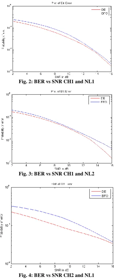
[image:4.595.320.522.72.222.2]The equalization model is analysed for BFO and DE based update algorithms and for this performance analysis de/rand/1 variation is used.
Fig. 2: BER vs SNR CH1 and NL1
Fig. 3: BER vs SNR CH1 and NL2
Fig. 4: BER vs SNR CH2 and NL1
Fig. 5: BER vs SNR CH2 and NL2
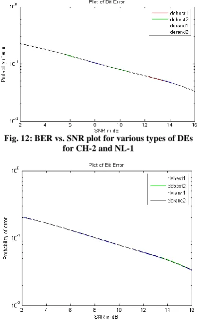
[image:4.595.77.276.214.699.2]The performance of DE based algorithm is better in comparision to BFO based algorithm which is evident from Fig.2 to Fig.5. Hence in the present work effect of various mutation startigies used in various types of DEs on channel equalization problem is also carried out. For this study four variants of DE based algorithms are used which are described mathematically in equations (4) to (7). For all four kinds of DEs the MSE floor for both CH1 and CH2 for NL1 and NL2 are ploted in Fig. 6 to Fig. 9 and then the BER vs. SNR plot are ploted in Fig. 10 to Fig. 13.
Fig. 6: MSE floor for various types of DE based Learning algorithm for CH1 and NL1
[image:4.595.320.518.372.643.2]Fig. 8: MSE floor for various types of DE based Learning algorithm for CH2 and NL1
Fig. 9: MSE floor for various types of DE based Learning algorithm for CH2 and NL2
[image:5.595.68.283.69.733.2]Fig. 10: BER vs. SNR plot for various types of DEs for CH-1 and NL-1
[image:5.595.318.522.72.406.2]Fig. 11: BER vs. SNR plot for various types of DEs for CH-1 and NL-2
Fig. 12: BER vs. SNR plot for various types of DEs for CH-2 and NL-1
Fig. 13: BER vs. SNR plot for various types of DEs for CH-2 and NL-2
5.
CONCLUSION
6.
REFERENCES
[1] John G. Proakis, “Digital Communication (Forth Edition)”Publishing House of Electronics Industry Beijing 2004
[2] B. Widrow and S. D. Stearns, Adaptive Signal Processing, chapter-6, pp. 99-116, Second Edition, Pearson.
[3] M.Reuter, J.Zeidler, “Nonlinear Effects in LMS Adaptive Equalizers”,IEEE Trans. Signal Processing, Vol.47, pp.1570-1579, June 1999 [4] S. Chen and B. Mulgrew, “Overcoming co-channel
interference using an adaptive radial basis function equalizer”, Signal Processing, Vol. 28, No. 1, 1992, pp. 91-107.
[5] J. C. Patra, R. N. Pal, R. Baliarsingh and G. Panda, “Nonlinear channel equalization for QAM signal constellation using Artificial Neural Network,” IEEE Trans. On Systems, Man and Cybernetics – Part B: vol. 29, No. 2, pp.262-272, April 1999. [6] M. Meyer and G. Pfeiffer, “Multilayer perceptron
based decision feedback equalizers for channels with intersymbol interference”, Proc.IEEE, Vol. 140, Pt. I, No. 6, December 1993, pp. 420-424. [7] D.J. Krusienski, W.K. Jenkins, The application of
particle swarm optimization to adaptive IIR phase equalization, in: ICASSP, vol. 2, May 2004, pp. 693–696.
[8] H. Sun, G. Mathew and B. Farhang-Boroujeny, “Detection techniques for high density magnetic recording”, IEEE Trans. on magnetics, vol.41, no. 3, pp. 1193-1199, March 2005
[9] G. J. Gibson, S. Siu and C. F. N. Cowan, “The application of nonlinear structures to t reconstruction of binary signals”, IEEE Trans. Signal processing, vol. 39, no. 8, pp. 1877-1884, Aug. 1991.
[10] Q. Liang and J. M. Mendel, “Equalization of nonlinear time-varying channels using type-2 fuzzy adaptive filters” IEEE Trans. Fuzzy Systems, vol. 8, pp. 551-563, Oct. 2000.
[11] E. Biglieri, A. Gersho, R.D. Gitlin, T.L. Lim, Adaptive cancellation of nonlinear intersymbol interference for voice-band data transmission, IEEE JSAC SAC-2 (5) (1984) 765–777.
[12] K. M. Passino, “Bio-mimicry of Bacterial Foraging for distributed optimization and control”, IEEE control system magazine, vol 22, issue 3, pp. 52-67, June 2002.